Sample Size Study of Driving Simulator Experiment for Freeway Design Safety Evaluations

Abstract

Driving Simulator, a powerful simulation tool, has already been used in safety evaluation of roadway geometric design during the pre-construction design stage. Conventional ways of estimating proper sample size include the empirical method, the resource equation, power analysis, and the Bayesian method. However, significant boundaries and prior distributions of operational indices are hard to identify in simulator studies, which makes it difficult to use conventional ways in choosing the acceptable sample size. This study proposes an empirical method to infer proper sample size. The Tongji University eight-degree-of-freedom driving simulator was utilized to collect continuous driving behavior data from a simulated mountainous freeway. Vehicle speed and lane departure events were selected as the indices to measure the influence of geometric design features on operational efficiency and safety. A mixed linear model and a mixed logistic regression model were used to assess the relationships between geometric design features and vehicle speed and lane departure. Random sampling was used to choose 10 samples of 5 to 50 drivers from a total of 55 drivers. Acceptable sample size was determined based on the parameter coefficient convergence elbow points of the mean squared error (MSE) curves of significant variables. The clear elbow points of the MSE curves indicate that 30 is an acceptable sample size.

Keywords

data and data science statistical methods pedestrians bicycles human factors road user measurement and evaluation simulator studies

Driving simulators are used effectively in roadway design safety evaluation. In Europe and the United States (U.S), driving simulators have been used in the design and visualization of roadways ( 1 , 2 ). In the U.S., Europe, Australia, and New Zealand, to name just a few, driving simulators have been used to measure the impact of various roadway design countermeasures on different kinds of driving performance from the safety of a laboratory ( 3 ). In China, the Specification for Highway Safety Audit recommends using driving simulators in complex road alignment safety evaluation ( 4 ).

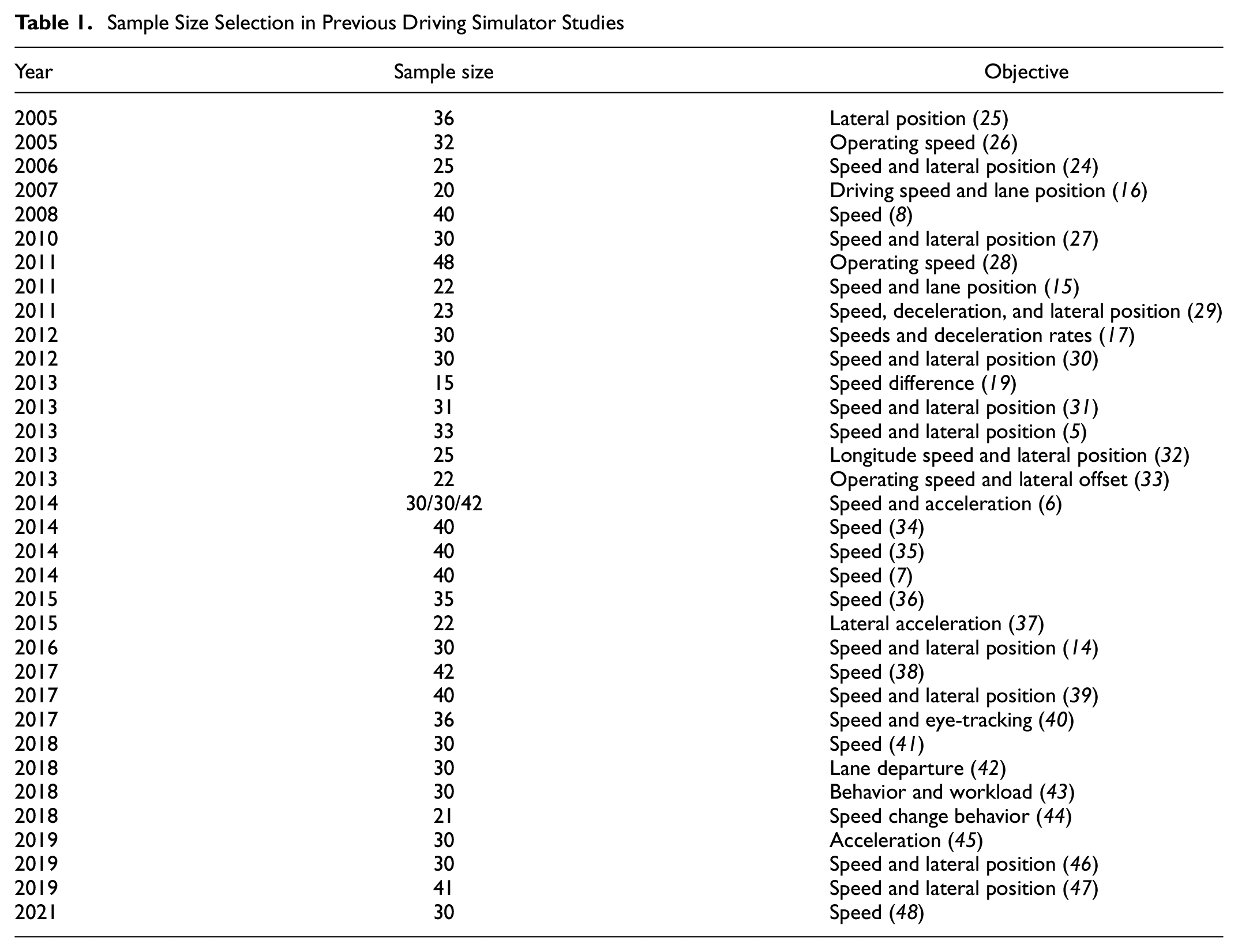
For simulator studies, sample size determination is crucial but hard in experiment design. An under-sized experiment is not able to provide researchers with credible results, while an over-sized experiment is expensive. The selections of sample size are usually a compromise of necessity, cost, and time. In previous studies, sample sizes were usually decided empirically without detailed discussion and quantitative analysis ( 5 – 8 ). Among the 34 papers reviewed in this study, where sample sizes varied from 15 to 48, none of them gave an explicit explanation of sample size determination. Therefore, proposing a quantitative method to calculate the smallest acceptable sample size is essential in driving simulator studies, as there are limitations on the number of participants which can be recruited because of resource constraints such as time and money ( 9 ).

Conventional statistical methods for determining sample size include: empirical methods; resource equations; power analysis with pre-assumed confidence intervals, power, and standard deviation (SD); and Bayesian methods with prior distributions ( 10 ). However, significant boundaries and prior distributions of operational indices are not easily identified in simulator studies, which makes it difficult to apply power analysis or Bayesian methods to choose the acceptable sample size. To solve this problem, this study proposes an empirical method, based on the parameter coefficient convergence elbow point of selected variables measured by mean squared error (MSE), to find the acceptable sample size.

This study developed two mixed effects models to assess driving behavior on combined alignments on a mountainous freeway. Fifty-five drivers’ data were collected to create a sufficiently large overall sample to permit different smaller sample sizes to be extracted from the pool to compare their model fitness. A random sampling method was employed to select sample sizes from 5 to 50 drivers; that is, the pool was randomly sampled 10 times for each of 10 sample sizes, with 5 drivers added to each subsequent sample size.

The parameter coefficient convergence elbow point of each selected variable was investigated with boxplots and MSE curves. Convergence was measured by the change of MSE for every parameter coefficient as the sample size increased, and was reached when the MSE curve elbow point appeared. Stability was measured by sample variance implied in the boxplots and inferred using the elbow method. The Wilcoxon signed-rank test was applied to examine whether the difference existed between sample sizes if there were more than one possible acceptable sample size inferred from the MSE curve. A smallest acceptable sample size was determined to be acceptable when both convergence and stability were realized.

This study takes into consideration the possible influence of model structure, estimation approach, and data distribution on sample size estimation from the elbow method convergence trend. Different types of model structures and estimation approaches were tested for different data fitting. Elbow points of MSE plots in the proposed method show that 30 is the minimum sample size for various model structures and estimation approaches.

Literature Review

Conventional Statistical Methods for Determining Sample Size

Conventional statistical methods for determining sample size include empirical methods, the resource equation, power analysis, and the Bayesian method ( 11 ). Statistical analysis is applied to determine the significant difference between the means or proportions observed in two or more comparison groups ( 12 ).

Empirical Methods

Many investigators are inclined to use the same sample size that has been confirmed effective in other similar work. Cox and Reid pointed out that the sample size is related to the experiment type, independent and dependent variables, experimental units, outcome variables, and so on ( 13 ).

For simulator studies, three papers used 40 drivers with ages ranging from 23 to 60, with 60% male participants and 40% female, and claimed that participant features were consistent with those of participants used in the previous study ( 5 – 8 ). Wu et al. conducted a simulator experiment beginning with 36 participants, though only 30 participants’ data were valid at the end ( 14 ). Four similar studies in road infrastructure are summarized in this paper that have sample sizes of 22 participants, 36 participants, and 30 participants ( 15 – 17 ).

Since no solid statistical analysis of sample size for driving simulator experiment design is given in these papers, the sample size of these papers cannot be directly considered reasonable without further analysis.

The Resource Equation

This method is widely used in the agricultural and industrial literature, as shown in Equation 1 ( 18 ). Singh and Masuku used a similar equation and gave a clear description of each parameter of the equation, and then proceeded to offer an example ( 12 ):

E = N - T

(1)

where

N = the total number of individuals in the study (minus 1),

T = the treatment component, corresponding to the number of experimental groups (minus 1), and

E = the degrees of freedom of error component.

Singh and Masuku concluded that, to achieve a better experiment effect, the value of E should range from 10 to 20. For example, if a study had a sample size of 32 (N = 31) and was divided into four treatment groups (T = 3) of eight participants each, then E would be equal to 28, which is higher than the cutoff of 20, indicating that the sample size might be a bit large and six participants per group might be more appropriate.

We reviewed 34 papers on the driving simulator experiments of freeway design safety evaluations and examined the values of all indicators: only one paper had the degrees of freedom of error component less than or equal to 20 ( 19 ). Thus, this method does not apply to us.

Power Analysis

In power analysis, the sample size can be estimated by the other five variables: effect size (ES), SD, power, significance level, and sidedness of the test ( 20 ).

The ES is the smallest mean difference between two study groups that the experimenter wants to detect. Previous experiments can help us estimate the SD of the character of interest. The power is the probability that the experiment will reject the null hypothesis when it is false. A power of 80% or 90% is usually specified. The significance level is the probability of rejecting the null hypothesis when the null hypothesis is true (determined by citing an α level). It is customarily set to 5%. Since the mean of the treated group could be either larger or smaller than the mean of the control group, a two-sided test is usually used. In some cases, it may be known before the investigation that any differences between the treated or control group may exist in only one direction. In such cases, one-sided statistical analysis can be considered ( 11 ).

In the current study, operation speed and lane departure cannot be obtained before the driving simulator experiment. Consequently, the variance of the response, the desired significance level, and the desired power of the operational indices present challenges because of the lack of significant boundaries of operational indices. Therefore, power analysis cannot be applied.

Bayesian Method

$θ ϵ Θ$ and $f (θ)$ are defined as the parameter of interest and the prior distribution for $θ$ , respectively. $Θ$ is the range where θ is computable. $x = (x_{1}, x_{2}, x_{3}, \dots, x_{n})$ is the sample of sample size n, x is the data space, $f (θ | x)$ . Let $f (x) = \int f (x | θ) f (θ) d θ$ represent the predictive marginal distribution of the data. For any given x, $f (θ | x) = f (x | θ) f (θ) / f (x)$ denotes the posterior distribution for $θ$ . In the Bayesian method, for a fixed posterior interval length l, the sample size can be determined by finding the smallest n that satisfies the inequation (2) as shown below in Equation 2. Therefore, the prior distribution is required at a given level $α$ when using the Bayesian approach ( 9 ).

\int {\int_{a}^{a + l} f (θ | x, n) d θ} f (x) dx \geq 1 - α

(2)

In the current study, the corresponding indices, such as SD and prior distribution, cannot be acquired before the driving simulator experiment has been conducted. Besides, making assumptions on the prior distribution of the Bayesian sample size estimation approach is not possible.

To sum up, conventional statistical methods for determining the sample size are not applicable in simulator studies. Power analysis demands pre-assumptions of the size of the response researchers want to detect, the variance of the response, the desired significance level, and the desired power. The Bayesian approach requires the identification of the prior distribution based on existing information ( 21 ). The equations and parameters of conventional statistical methods for determining sample size can be found in the Appendix in Table A.

Indices Adopted in Driving Simulator Application on Roadway Alignment Design

Poorly designed combined (vertical and horizontal) alignments cause a deterioration of freeway safety ( 22 , 23 ). In real applications, identifying alignment problems in the design stage is more efficient than identifying them after construction. Thus, driving simulators have been widely used as the main tools for proactively examining roadway alignment designs. This study reviewed 34 papers from 2005 to 2021 that used driving simulators to investigate roadway design safety. As summarized in Table 1, speed and lateral position are the most frequently used surrogate measures ( 15 , 16 , 24 ).

Table 1.

Sample Size Selection in Previous Driving Simulator Studies

Year	Sample size	Objective
2005	36	Lateral position ( 25 )
2005	32	Operating speed ( 26 )
2006	25	Speed and lateral position ( 24 )
2007	20	Driving speed and lane position ( 16 )
2008	40	Speed ( 8 )
2010	30	Speed and lateral position ( 27 )
2011	48	Operating speed ( 28 )
2011	22	Speed and lane position ( 15 )
2011	23	Speed, deceleration, and lateral position ( 29 )
2012	30	Speeds and deceleration rates ( 17 )
2012	30	Speed and lateral position ( 30 )
2013	15	Speed difference ( 19 )
2013	31	Speed and lateral position ( 31 )
2013	33	Speed and lateral position ( 5 )
2013	25	Longitude speed and lateral position ( 32 )
2013	22	Operating speed and lateral offset ( 33 )
2014	30/30/42	Speed and acceleration ( 6 )
2014	40	Speed ( 34 )
2014	40	Speed ( 35 )
2014	40	Speed ( 7 )
2015	35	Speed ( 36 )
2015	22	Lateral acceleration ( 37 )
2016	30	Speed and lateral position ( 14 )
2017	42	Speed ( 38 )
2017	40	Speed and lateral position ( 39 )
2017	36	Speed and eye-tracking ( 40 )
2018	30	Speed ( 41 )
2018	30	Lane departure ( 42 )
2018	30	Behavior and workload ( 43 )
2018	21	Speed change behavior ( 44 )
2019	30	Acceleration ( 45 )
2019	30	Speed and lateral position ( 46 )
2019	41	Speed and lateral position ( 47 )
2021	30	Speed ( 48 )

Speed, especially free-flow speed, is frequently used to evaluate operational safety. Continuous operating speed profiles are good measures of the general interaction between drivers and the roadway design ( 8 ). Lane departure event, identified as extremely large lateral lane departures, is another critical safety surrogate, which has been used as a predictive variable in many studies of single vehicle run-off-road (ROR) crashes ( 16 , 42 , 49 ). Torbic et al., for instance, found that approximately 76% of curve-related fatal crashes were single-vehicle ROR crashes ( 50 ).

Sample Size of Driving Simulator Experiments for Freeway Design Safety Evaluations

Determining whether the sample size is adequate, that is, the smallest, in performing a reliable statistical analysis in freeway design safety evaluations, greatly saves cost and time when doing driving simulators studies. Nevertheless, none of the 34 investigated studies, shown in Table 1, present quantitative arguments that justify their choice of a given in sample size for their experiment. The chosen sample sizes for these studies varied from 15 to 48 drivers: 40 or more samples were used in nine papers, 30 to 40 were used in 16 papers, and fewer than 30 samples were used in nine papers.

The determination of adequate sample size in driving simulator studies with constraints on the number of participants is still nascent ( 21 ). This is particularly true of roadway safety evaluation. Chen et al. were the first researchers to use statistical methods to determine an acceptable sample size in driving simulator studies of geometric design where hard limitations exist on the sample size ( 42 ). They employed a quantitative measure which applied a t-test in the comparison of the results of all 30 drivers and 27 male drivers (included in the 30 drivers sample pool) ( 42 ). As no difference between various sample sizes was detected through the t-test, they chose to use the model developed from the 27 male drivers for the parsimonious rule of cost saving ( 42 ). This selection appears to be assertive because no distinct differences were detected in their study.

As noted in previous sections of this paper, speed and lane departure are the most frequently used surrogate measures in roadway design safety evaluation. In this case, the operation speed and the characteristics of lane departure cannot be obtained before the driving simulator experiment, since the road is still in the design stage. Consequently, the confidence interval and SD of the operational indices cannot be determined, which makes it difficult to apply traditional methods to choose the acceptable sample size ( 9 ). To solve this problem, this study proposes an empirical method, based on the parameter coefficient convergence of selected variables measured by MSE, to find the acceptable sample size.

Data Preparation

Equipment

The Tongji University driving simulator (see Figure 1) has an eight-degree-of-freedom motion system with an X-Y range of 20 × 5 m. The simulator cabin is a closed dome with a fully instrumented Renault Megane III vehicle in the center. The complete force feedback system of the steering wheel, pedals, and gears provides a responsive driving experience, and the visual system, which includes five projectors and three LCD monitors, adds to the recorded data. The immersive five-projector system provides a front image view of 250° × 40° at 1,400 × 1,050 × 5 pixels resolution refreshed at 60 Hz, and the LCD monitors give rear views of the central and side mirrors. Numerous experiments evidence that the Tongji University driving simulator reliably collects driving behavior data with its steady and realistic driving scenarios ( 33 ).

Figure 1.

Tongji University driving simulator: (a) driving simulator, (b) vehicle, and (c) driver view.

Studied Freeway Configuration

The simulated driving scenario was based on a section of the Yongji Freeway, a mountainous freeway in Hunan Province, China. The section is a 24 km four-lane roadway with a longitudinal grade ranging from −6.0% to +4.0%, and a horizontal curve radius ranging from 400 m to 2,000 m. The steepest −6.0% slope appears in the bridge section of Yongji Freeway with a speed limit of 80 km/h, while the design speed for other parts is 100 km/h. A cross-section profile of the simulated roadway is shown in Figure 2 and the aerial view of the simulated freeway is shown in Figure 3.

Figure 2.

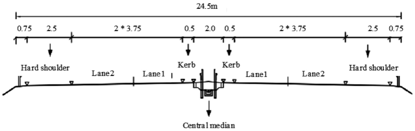
Road cross-section.

Figure 3.

Aerial view of the simulated freeway.

Driver Recruitment

A stratified sampling method was used to choose a random sample proportional to the male and female driver ratio in China, which is around 5:1. Criteria for participant selection included their having driven at least 10,000 km and having an average mileage of at least 3,000 km annually. Apart from driving experience and gender, drivers’ age was also considered to generally conform to the distribution of the driving population. The drivers’ ages ranged from 23 to 57 with an average age of 33 and a SD of 9.1. A physiological survey was conducted after the experiment, to assess possible simulator sickness; it consisted of four levels: no feeling of sickness, mildly sick, moderately sick, and severely sick ( 44 ). Driving data was excluded if any level of sickness was detected during the experiment. As a result, 55 of the original 57 recruited drivers completed the experiments successfully; the basic information about them is summarized in Table 2.

Table 2.

Participating Drivers

Category	Count	Percentage
Gender
Male	46	83.6
Female	9	16.4
Age
<35	33	60.0
≥35	22	40.0
Driving experience
<4 years	17	30.9
≥4 years	38	69.1

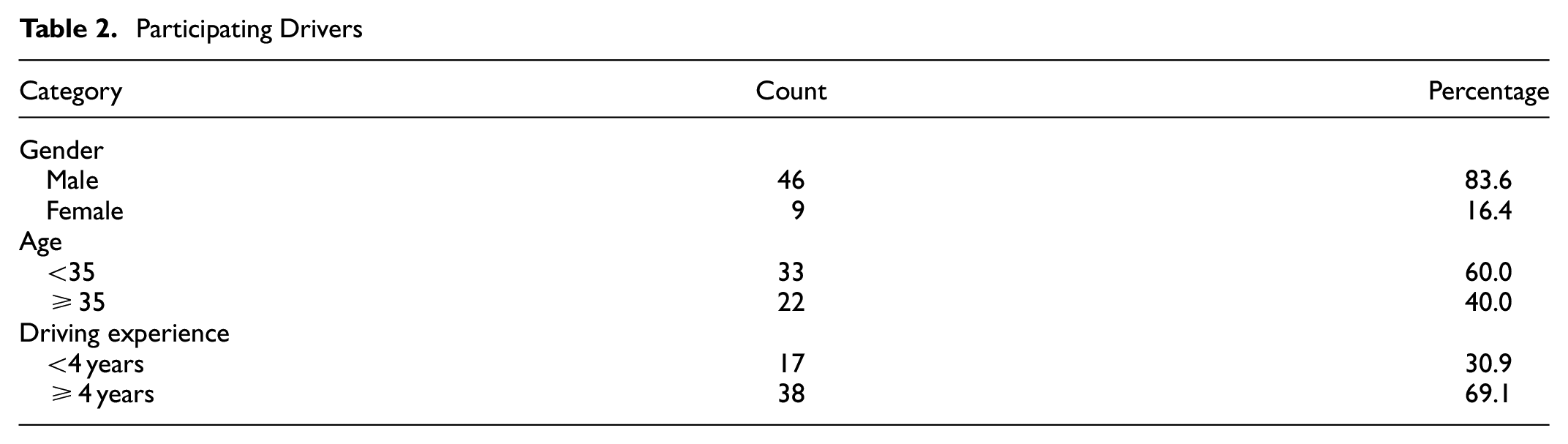
The participants’ driving experience criteria is based on the papers for driving simulator research of roadway design safety evaluation. Previous studies (e.g., Bella, Domenichini et al., and Bella and Silvestri) selected the participants according to the following characteristics: at least 4 years of driving experience and an average annual driven distance of at least 2,500 km ( 7 , 8 , 38 , 39 ). Then, the total mileage of the participants was at least 10,000 km. Calvi and Bella, and Bella et al. required the participants’ annual mileage to be at least 3,000 km ( 34 , 35 ). Therefore, another selection criteria included participants having driven at least 10,000 km and having an average mileage of at least 3,000 km annually.

Experimental Procedures and Design

To eliminate possible interference from traffic and environment and to focus on geometric design variables, the driving scenarios were set under free flow conditions, in daylight, and on dry pavement. The experimental sessions consisted of three phases: preparation, warm-up, and test. During the preparation phase, drivers filled in their personal information and were informed of the research purpose, potential risks, and operation of the simulator vehicle. In the warm-up phase, the drivers spent 10 min driving in other simulation scenarios to get familiar with the operational characteristics of the simulator. In the test phase, each participant drove the 24 km length of the study freeway in a single continuous run, immediately followed by driving in the opposite direction.

Driving Data Collection

Following previous work on roadway design safety evaluation, speed and lane departure were the main focus of this study. Speed is a good reflection of a vehicle’s longitudinal performance. Lane departure is determined by the lateral lane shift of the vehicle ( 33 , 42 ). Lateral lane shift is the distance between the lane’s center line and the vehicle’s center line—lane departure was identified when lateral shift exceeded 77.5 cm. A schematic diagram illustrating lane departure is shown in Figure 4.

Figure 4.

Schematic diagram of a lane departure scenario: (a) diagram of a lane departure scenario and (b) calculation of lateral lane offset thresholds.

The driving simulator collects data at a frequency of 20 Hz. To compare different drivers at the same locations, the 24 km road section was divided into short equidistant segments of 5 m. Vehicle operation measures of speed and lane departure collected on the first and last kilometers of the studied road were excluded because of the potential inaccuracy caused by the vehicles’ acceleration and deceleration at these points.

Collection of Geometric Design Characteristics

To predict this study’s variables of speed (a continuous variable) and occurrence of lane departure (a binary variable), geometric parameters were collected from 400 m, 300 m, 200 m, 150 m, 100 m, and 50 m adjacent segments upstream and downstream from the driver, as well as from the roadway’s combined alignments of the current segment. The idea of this modeling strategy is that vehicle operation measures taken by drivers at the current combined alignment are influenced by their experience along the roadway (upstream) segment and their expectations based on the viewable upcoming (downstream) segment (Figure 5) ( 42 ). The stopping sight distance (SSD) is 72.50 m (from the SSD equation provided in the U.S.’s Green Book A Policy on Geometric Design of Highways and Streets) ( 23 ). The authors used a 50 m interval for convenience during data preparation.

Figure 5.

Current, upstream, and downstream segments.

Since the alignment of the two directions is not completely consistent, the operation data used in the paper was the one-sided driving data from south to north. Various geometric characteristics were extracted as independent variables. From the current segment, grade, direction, and curvature were collected. From adjacent segments, average grade, tangent-proportion, and maximum change in slope were collected. Descriptive statistics for the roadway’s current and adjacent segments are listed in Tables 3 and 4.

Table 3.

Continuous Variables of Geometric Design Characteristics

	Variables	Description	Mean	Standard deviation	Min.	Max.
Current segments	$Curvature$	Curvature of current segment	0.0007	0.0007	0	0.0025
Current segments	Slope	Slope of current segment	−0.00584	0.025	−0.06	0.06
Adjacent segments (e.g., upstream 400 m segment)	AvgSU400	Mean slope of upstream 400 m segment	−0.0064	0.0214	−0.06	0.0351
	$Δ S_{U 400}$	Slope differential of max. and min. value of upstream 400 m segment	0.0233	0.0205	0	0.081
	AvgCU400	Mean curvature upstream 400 m segment	0.0007	0.0006	0	0.0024
	DiffCU400	Curvature differential of max. and min. values of upstream 400 m segment	0.0015	0.0013	0	0.005
	DownPU400	Down slope proportion of upstream 400 m segment	0.3044	0.3361	0	1
	$Tangent_P_{U 400}$	Straight proportion of upstream 400 m segment	0.3874	0.3992	0	1
Adjacent segments (e.g., downstream 400 m segment)	AvgSD400	Mean slope of downstream 400 m segment	−0.0059	0.0214	−0.06	0.0350
	$Δ S_{D 400}$	Slope differential of max. and min. value of downstream 400 m segment	0.0231	0.0205	0	0.081
	AvgCD400	Mean curvature downstream 400 m segment	0.0007	0.0006	0	0.0024
	DiffCD400	Curvature differential of max. and min. values of downstream 400 m segment	0.0015	0.0013	0	0.005
	DownPD400	Down slope proportion of downstream 400 m segment	0.3009	0.3370	0	1
	$Tangent_P_{D 400}$	Straight proportion of downstream 400 m segment	0.3874	0.3992	0	1

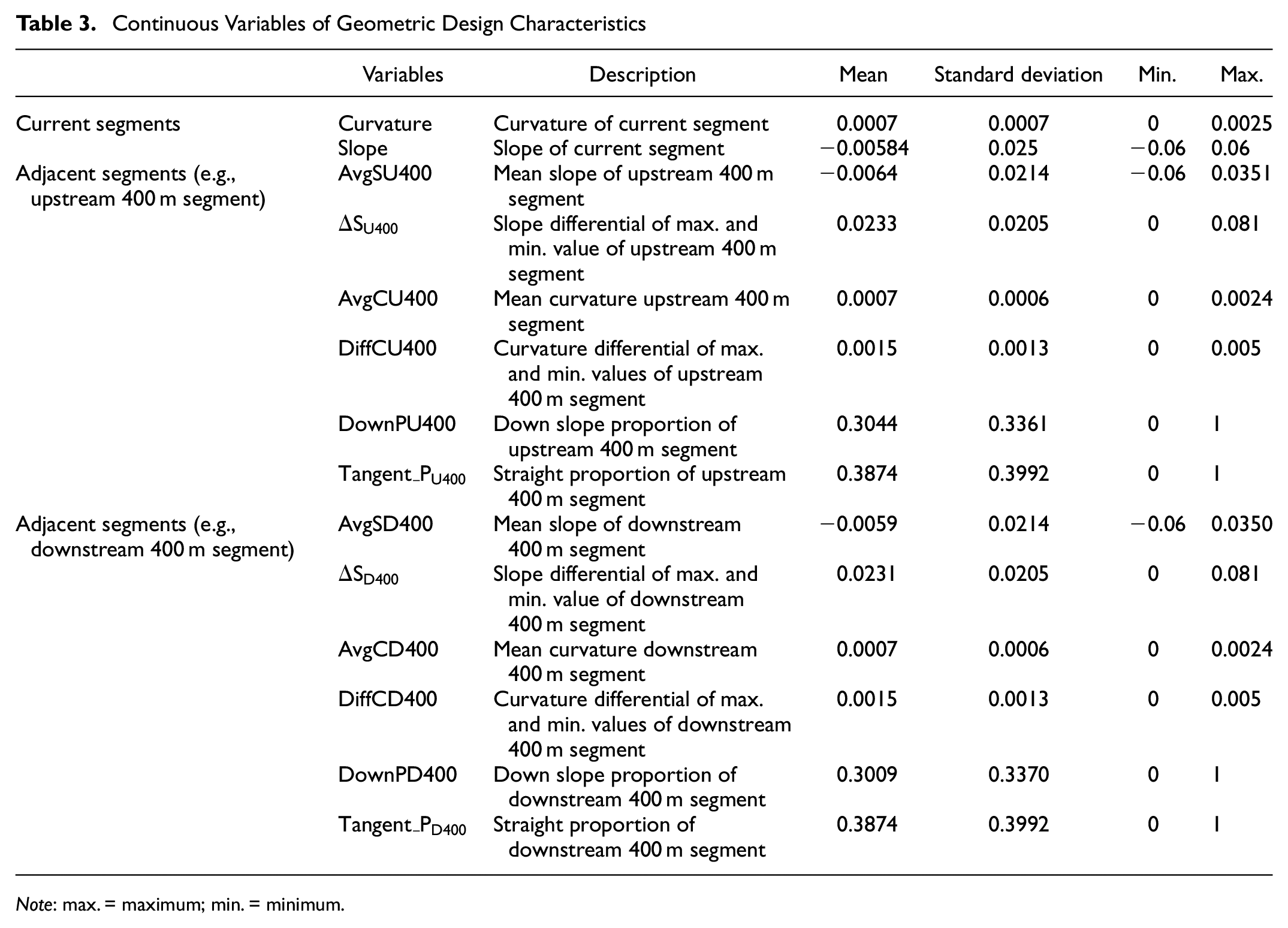
Note: max. = maximum; min. = minimum.

Table 4.

Categorical Variables of Geometric Design Characteristics

	Variables	Group	Value	Percentage
Current segments	$S_{type}$ (slope type)	Downslope: slope < −0.03	−1	15.3
		Flat: −0.03 < slope < 0.03	0	79.2
		Upslope: slope > 0.03	−1	5.5
	Direction (direction type)	Straight	0	38.7
		Turn left	1	30.2
		Turn right	2	31.0
	$H_{type}$ (alignments type)	Straight	1	38.7
		Circle curve	2	32.0
		Approach transition	3	14.7
		Depart transition	4	14.6
Adjacent segments (e.g., Upstream 400 m segment)	$SD_L_{U 400}$ (slope difference)	=0	0	33.02
		0–0.02	1	12.45
		0.02–0.04	2	28.81
		> 0.04	3	25.72
	$Reverse_C_{U 400}$ (reverse curve)	No	0	63.71
	$Reverse_C_{U 400}$ (reverse curve)	Yes	1	36.29
	$MaxC_L_{U 400}$ (max curvature)	=0	0	19.11
		0–0.0014 and radius > 700 m	1	41.85
		>0.0014 and radius < 700 m	2	39.04

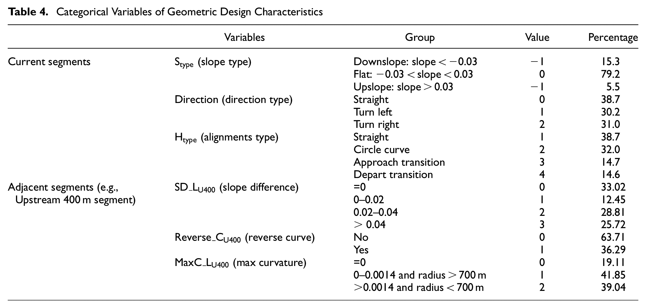
As shown in Tables 3 and 4, there are three categorical variables divided by threshold, slope type of current segment, slope difference of adjacent segment, and maximum curvature of adjacent segment. The threshold of the three variables were defined in consideration of Specification for Highway Safety Audit and Design Specifications for Highway Alignment in China ( 4 ). The principles adopted are summarized as follows:

1) Slope type

According to B.2.1 Division of analysis unit of Specification for Highway Safety Audit in China, the gradient of 3% was used as the threshold value for dividing the straight road section and longitudinal slope section ( 4 ). Therefore, the slope-type was divided into three groups: downslope (grade less than −3%), level (grade between −3% and 3%), and upslope (grade greater than 3%).

2) Slope difference

According to 8.2 Slope of Design Specification for Highway Alignment in China, when the design speed is 100 km/h, the grade should be flatter than 4% ( 51 ). In addition, considering the distribution of slope, the slope difference was divided into four groups: 0, 0%–2%, 2%–4%, and >4%.

3) Maximum curvature

According to 7.3 Circular curve of Design Specification for Highway Alignment in China, the minimum radius of the circular curve with 100 km/h design speed for freeway is recommended to be 700 m ( 51 ). Therefore, the MaxCurvature-typeF400 was divided into three groups: 0, 0–0.0014, and >0.0014.

Methodology

Random Intercept Model

As noted, speed and lane departure reflect driving stability longitudinally and laterally. In our study, speed and lane departure behavior data from a driving simulator experiment were modeled to establish the relationships between these behaviors and roadway geometric design. Considering that heterogeneity may arise from individual differences in modeling, drivers’ individual effects were treated as random effects, accordingly ( 44 ). A mixed linear model was used to investigate the relationship between geometric design and speed, and a mixed logistic regression model was used to investigate the effects of design on lane departure.

Equation 3 displays the formula for the mixed linear model to measure the relationship between speed and geometric design:

v_{ij} = Σ_{j = 1}^{n} α_{C} X_{C} + Σ_{kU = 1}^{n} α_{kU} X_{kU} + Σ_{kD = 1}^{n} α_{kD} X_{kD} + ε_{ij}^{*}

(3)

where

$v_{ij}$ = the speed of driver $i$ at segment j,

$X_{kU}$ and $X_{kD}$ = the geometric characteristics of the adjacent segments (several alternative segment ranges (k = 50, 100, 150, 200, 300, 400) were compared by model fitness to decide the optimal range for evaluating their influence on speed),

$ε_{ij}^{*}$ = the random effect of driver $i$ at segment j, and

$ε_{ij}^{*}$ = $NID (0, σ^{2})$ .

A mixed logistic regression model was used to measure the relationship between lane departure and geometric design. Probabilities were estimated using a logistic function where the log-odds of the probability of moving out of a lane is the linear combination of predicting variables ( 52 ). Occurrence of lane departure was set as the dependent variable with two possible values of 0 and 1, with 0 referring to staying in the lane, and 1 referring to moving out of the lane.

\begin{matrix} \log \frac{P (Y_{ij} = 1)}{P (Y_{ij} = 0)} = Σ_{j = 1}^{n} β_{C} X_{C} + Σ_{kU = 1}^{n} β_{kU} X_{kU} \\ + Σ_{kD = 1}^{n} β_{kD} X_{kD} + μ_{ij} \end{matrix}

(4)

where

$P (Y_{ij} = 1)$ = the probability that driver $i$ moves out of the lane at segment j, and

$μ_{ij}$ = the random effect for the driver’s individual effects on parameter coefficient estimation (which is assumed to follow standard normal distribution with a mean of 0 and constant variance).

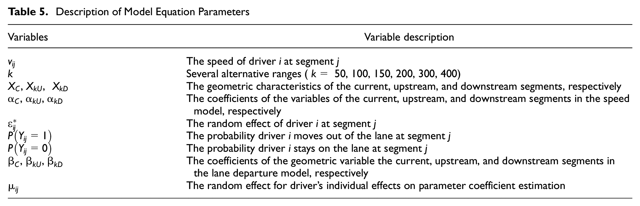
A description of model equation parameters is summarized in Table 5.

Table 5.

Description of Model Equation Parameters

Variables	Variable description
$v_{ij}$	The speed of driver $i$ at segment j
$k$	Several alternative ranges ( $k =$ 50, 100, 150, 200, 300, 400)
$X_{C}$ , $X_{kU}$ , $X_{kD}$	The geometric characteristics of the current, upstream, and downstream segments, respectively
$α_{C}$ , $α_{kU}$ , $α_{kD}$	The coefficients of the variables of the current, upstream, and downstream segments in the speed model, respectively
$ε_{ij}^{*}$	The random effect of driver $i$ at segment j
$P (Y_{ij} = 1)$	The probability driver $i$ moves out of the lane at segment j
$P (Y_{ij} = 0)$	The probability driver $i$ stays on the lane at segment j
$β_{C}$ , $β_{kU}$ , $β_{kD}$	The coefficients of the geometric variable the current, upstream, and downstream segments in the lane departure model, respectively
$μ_{ij}$	The random effect for driver’s individual effects on parameter coefficient estimation

Acceptable Sample Size Test

The primary purpose of this study was to determine optimal sample size for simulator research, considering factors such as time consumed, cost, and the level of necessity for data collection. A simple random sampling method was applied in this study to choose sample sizes ranging from 5 to 50 drivers. To maintain information while not increasing computing expenditure, the 55-driver pool was randomly sampled to arrive at 10 sample sizes in increasing 5-driver increments from 10 to 50, with all but the largest size having 10 separate random samples. The initial sample size is the largest one implemented to date in an experiment of this sort based on a meta-analysis of previous research. The sample size derived from an empirical method is unlikely to be larger than the initial sample size.

The elbow of the models’ estimated coefficients is a good indicator of acceptable sample size. Model coefficient convergence estimation should be quantitatively identified, since the elbow of a steady trend in parameter coefficients implies the appropriateness of a sample size ( 53 ). MSE averages the squares of the errors, and is typically used as a measure of estimate quality. MSE thus can be a good criterion by which to check the convergence of model coefficients estimation. A popularly used loss function is shown in Equation 5:

MSE = L (f (X), Y) = \frac{1}{n} \sum_{i = 1}^{n} {({\tilde{Y}}_{I} - Y_{i})}^{2}

(5)

where

$f (X)$ = is the parameter coefficient for a certain number of samples, and

Y = the parameter coefficient for our 55-driver pool.

The smaller the MSE, the more sufficient the sample size. Acceptable sample size is identified when convergence and stability are reached beyond the elbow point. The “elbow point” is a tipping point which denotes the trend is converged after this point no matter the size of the largest sample size that is being collected. Besides MSE, the stability of the estimated coefficients of the boxplot interquartile after the elbow point, as sample size increases, also can indicate the adequate sample size has been reached.

MSE and boxplots were, therefore, used in this study, and further investigation was conducted through the Wilcoxon signed-rank test to check the suitability of the sample size in comparison to the full-size models. The Wilcoxon signed-rank test, along with the Wilcoxon-rank sum test, were nonparametric tests proposed by Wilcoxon in 1945 for the one-sample location problem ( 54 ). The Wilcoxon signed-rank test is used to compare the equality of two paired dependent samples, and it is a nonparametric alternative to the paired Student’s t-tests ( 55 ). It does not assume the samples are normally distributed, which loosens the normality assumption that many dependent samples may not satisfy.

Acceptable Sample Size for Speed Model Analysis

The mixed linear model was used to establish the relationship between speed and geometric design features for the differently sized samples (Table 6). Speed was set as the dependent variable. The process of variable selection is as follows:

Insignificant variables with p-values less than 0.05 were removed from the total 113 variables included in the mixed linear speed model.

The stepwise method was then applied to select variables in the retained subset based on the Akaike information criteria (AIC).

After the stepwise regression, a variance of inflation (VIF) test was performed on the model with reserved variables; some had VIFs over 10, implying multicollinearity.

To remedy the multicollinearity, a least absolute shrinkage and selection operator (LASSO) regression was built by adding an optimal constant tuning parameter with the minimization of cross-validation error.

Variables with penalized coefficients of 0 were removed, and some highly correlated independent variables were dropped.

Variables were removed if they overlapped much in meaning with other variables, while more unique variables were retained in the final model.

Table 6.

Speed Model Coefficient Estimations for Different Sample Sizes

Sample size	Variables	Evaluation	Standard deviation	t-value	P-value	R-square*
55	Intercept	99.0872	1.4394	68.84	<.0001	0.039309
	Slope	−30.014	1.2254	−24.49	<.0001
	AvgSU400	−154.11	1.8919	−81.46	<.0001
	DownPU400	−3.3884	0.08468	−40.02	<.0001
	DownPD400	−2.0711	0.0616	−33.62	<.0001
	AvgCU400	−192.75	26.8761	−7.17	<.0001
50	Intercept	99.7395	1.5225	65.51	<.0001	0.041; 0.049; 0.043; 0.038; 0.037; 0.039; 0.038; 0.039; 0.044; 0.036
	Slope	−29.5935	1.2681	−23.34	<.0001
	AvgSU400	−151.41	1.9577	−77.34	<.0001
	DownPU400	−3.3142	0.08762	−37.82	<.0001
	DownPD400	−1.9997	0.06375	−31.37	<.0001
	AvgCU400	−220.35	27.8121	−7.92	<.0001
45	Intercept	99.5349	1.6131	61.71	<.0001	0.044; 0.037; 0.035; 0.051; 0.041; 0.038; 0.035; 0.036; 0.037; 0.064
	Slope	−32.0267	1.3571	−23.6	<.0001
	AvgSU400	−149.31	2.0952	−71.26	<.0001
	DownPU400	−3.3361	0.09378	−35.57	<.0001
	DownPD400	−2.0158	0.06822	−29.55	<.0001
	AvgCU400	−225.18	29.7646	−7.57	<.0001
40	Intercept	99.4581	1.7129	58.07	<.0001	0.050; 0.033; 0.031; 0.033; 0.036; 0.073; 0.034; 0.042; 0.030; 0.049
	Slope	−32.047	1.4661	−21.86	<.0001
	AvgSU400	−141.42	2.2634	−62.48	<.0001
	DownPU400	−3.3469	0.1013	−33.04	<.0001
	DownPD400	−2.0098	0.0737	−27.27	<.0001
	AvgCU400	−208.54	32.1542	−6.49	<.0001
35	Intercept	99.9193	1.7232	57.99	<.0001	0.053; 0.033; 0.045; 0.098; 0.034; 0.056; 0.047; 0.028; 0.023; 0.042
	Slope	−39.0183	1.4455	−26.99	<.0001
	AvgSU400	−150.78	2.2316	−67.56	<.0001
	DownPU400	−3.7151	0.09988	−37.2	<.0001
	DownPD400	−2.2341	0.07266	−30.75	<.0001
	AvgCU400	−196.4	31.7025	−6.2	<.0001
30	Intercept	100.12	1.8969	52.78	<.0001	0.050; 0.030; 0.041; 0.146; 0.026; 0.051; 0.056; 0.038; 0.022; 0.050
	Slope	−34.3749	1.6581	−20.73	<.0001
	AvgSU400	−147.32	2.5598	−57.55	<.0001
	DownPU400	−3.2306	0.1146	−28.2	<.0001
	DownPD400	−1.9756	0.08335	−23.7	<.0001
	AvgCU400	−198.54	36.3657	−5.46	<.0001
25	Intercept	101.31	1.3835	73.22	<.0001	0.058; 0.029; 0.040; 0.152; 0.023; 0.052; 0.060; 0.036; 0.017; 0.042
	Slope	−21.7793	1.5191	−14.34	<.0001
	AvgSU400	−238.29	2.3452	−101.61	<.0001
	DownPU400	−4.6357	0.105	−44.16	<.0001
	DownPD400	−1.3094	0.07636	−17.15	<.0001
	AvgCU400	−174.28	33.3165	−5.23	<.0001
20	Intercept	101.08	2.6557	38.06	<.0001	0.052; 0.022; 0.031; 0.220; 0.026; 0.061; 0.066; 0.039; 0.020; 0.055
	Slope	−21.6694	1.9235	−11.27	<.0001
	AvgSU400	−200.12	2.9695	−67.39	<.0001
	DownPU400	−4.457	0.1329	−33.53	<.0001
	DownPD400	−2.2006	0.09669	−22.76	<.0001
	AvgCU400	−324.88	42.1855	−7.7	<.0001
15	Intercept	103.09	3.1996	32.22	<.0001	0.045; 0.021; 0.039; 0.188; 0.041; 0.082; 0.089; 0.047; 0.017; 0.059
	Slope	−23.3031	2.3527	−9.9	<.0001
	AvgSU400	−160.22	3.6321	−44.11	<.0001
	DownPU400	−3.5367	0.1626	−21.76	<.0001
	DownPD400	−1.4086	0.1183	−11.91	<.0001
	AvgCU400	−329.89	51.5988	−6.39	<.0001
10	Intercept	105.3	4.7131	22.34	<.0001	0.050; 0.023; 0.031; 0.206; 0.088; 0.118; 0.097; 0.048; 0.021; 0.044
	Slope	−28.0432	3.0142	−9.3	<.0001
	AvgSU400	−222.2	4.6534	−47.75	<.0001
	DownPU400	−6.5992	0.2083	−31.68	<.0001
	DownPD400	−3.0311	0.1515	−20	<.0001
	AvgCU400	−279.46	66.1076	−4.23	<.0001

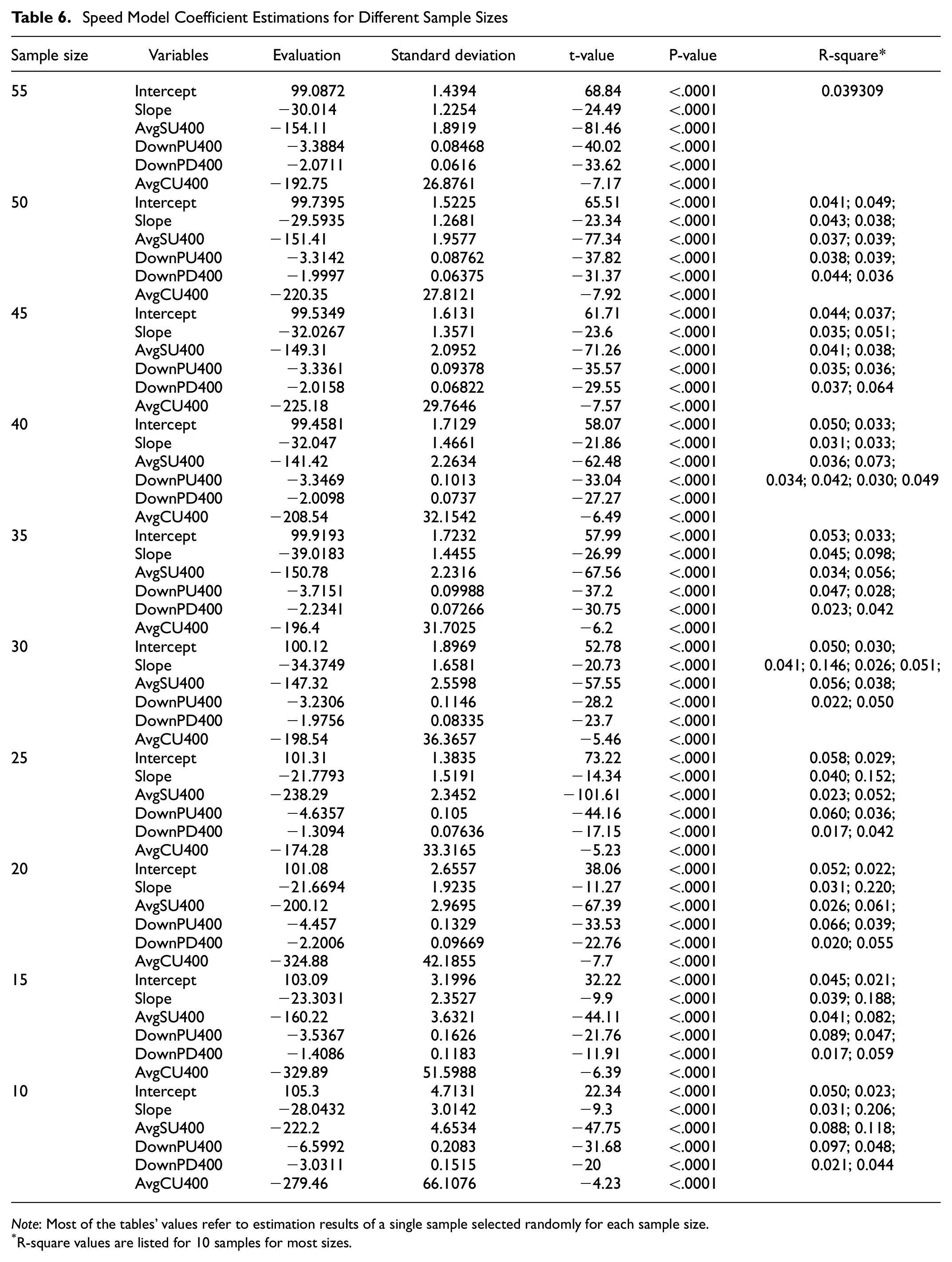
Note: Most of the tables’ values refer to estimation results of a single sample selected randomly for each sample size.

R-square values are listed for 10 samples for most sizes.

As a result, excessively overlapped variables (with correlation higher than 0.6) were removed, and slope, avgSU400, downPU400, downPD400, and avgCU400 were left in the final model. Data heterogeneity resulting from the discrepancies in driver behavior was handled by treating drivers as a random effect. To consider inflation, R-square was calculated by using a fixed-effects, mixed linear model, as shown below ( 56 ).

The significance of the random effect, the intercept of every model, implies that the existence of individual discrepancies is substantially related to the change of speed; thus, drivers’ individual differences cannot be neglected. It can be seen in Table 6 that all the mixed effect variables are significant for every sample size. Model interpretability becomes more trustworthy as sample size increased in the speed model analysis, as indicated by the stability of R-square. Values of R-square fluctuate between 0.019 and 0.172 for sample sizes less than 25, as listed in Table 6. The change of R-square approaches stability at sample sizes larger than 30.

Coefficients of intercept, slope, avgSU400, downPU400, downPD400, and avgCU400 were calculated by the random sampling method of selecting 5 drivers for every sample step 10 times. Boxplots were constructed to check the converging stability of each variable in different sample sizes, where variability is measured by interquartile and the bands inside the boxes represent the medians (Figure 6).

Figure 6.

Box-plot of speed model coefficient estimation of different sample sizes: (a) intercept, (b) slope, (c) avgSU400, (d) downPU400, (e) downPD400, and (f) avgCU400.

It can be seen in all six variables that, as sample size increased, fluctuations, or variability, of the estimated coefficients generally decreased. Stability can be inferred from the gradual attenuated fluctuations of the parameter coefficients, reflected in the steady change of interquartile and median. As Figure 6 shows, downPD400 reached stability quickly as sample size increased to 25, and slope and avgCU400 became stable when sample size increased to 30. AvgSU400 and downPU400 were the least sensitive to increase in sample size, where stability was achieved only at sizes over 30. Although the trends to convergence stability are not identical for all variables, converging patterns are apparent as sample size moves above 30.

Determination of acceptable sample size by boxplots is unsteady and lack of validation.Quantitative measurement methods rather than empirical approaches should be applied, such as MSE, which is typically used as a measure of estimator quality.

MSE is a good measure for loss function, which is based on the average of the squared of errors, and can be a good criterion to check the convergence of a model estimated coefficients. The converged point is the tipping point to indicate that patterns remain the same after the tipping point. Figure 7 depicts the change in MSE as sample size increased.

Figure 7.

Mean squared error (MSE) of each variable for different speed model sample sizes: (a) intercept, (b) slope, (c) avgSU400, (d) downPU400, (e) downPD400, and (f) avgCU400.

In Figure 7, distinct converging patterns are shown for the different variables. For example, avgSU400, downPD400, and avgCU400 converged quickly as sample size increased. Twenty-five drivers is considered to be the acceptable size for these four variables according to GRAPH ACEF. Slope and downPU400 display a slightly different converging style according to GRAPH BD: a steady trend appears first, but is followed with a further downtrend that converges at the size of 30. Figure 7 shows 30 as an acceptable sample size, since the converging trend exists by that point, even with GRAPH BD. However, sample size of 35 may also be the acceptable size to consider since the trend is more converged at 35. Sample sizes larger than 40 are not necessary to check because they are too close to the full size of 55.

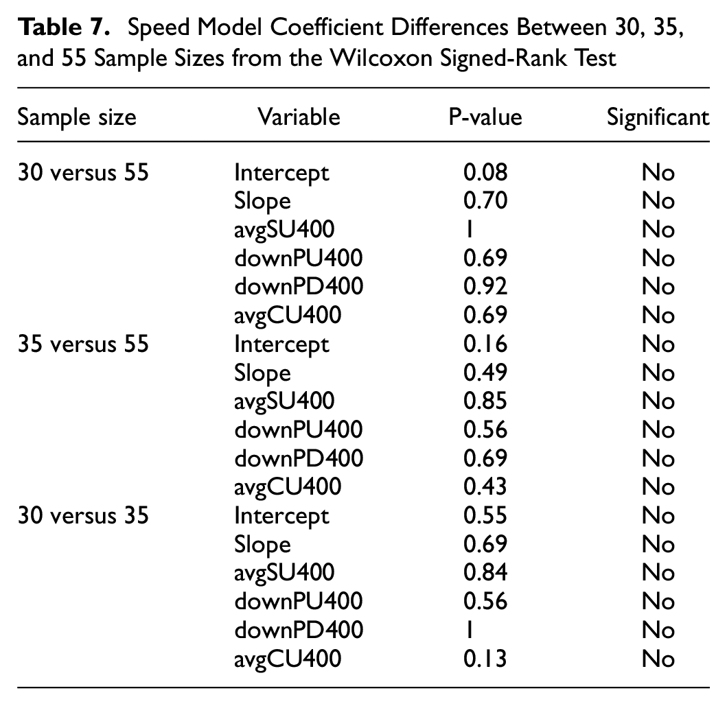
To check the acceptability of the sample size, the Wilcoxon signed-rank test was used to determine whether the coefficients of sample size 30 and sample size 35 significantly differ from coefficients for the full set of 55 drivers from speed model. The Wilcoxon signed-rank test is the nonparametric alternative to the paired Student’s t-tests that loosens the normality assumption for random error.

A lack of significant difference in a variable’s Wilcoxon signed-rank test indicates that no significant difference was detected for the variable between the two compared models of different sample sizes. If most of the variables’ values showed insignificant differences, then the two models were considered as identical. As shown in Table 7, neither the 30- nor 35-driver model was found to significantly differ from the full-size model, since all of the regressed variables were insignificant. Therefore, a sample size of 30 drivers should be sufficient for building a mixed linear regression speed model for the parsimonious rule of cost saving.

Table 7.

Speed Model Coefficient Differences Between 30, 35, and 55 Sample Sizes from the Wilcoxon Signed-Rank Test

Sample size	Variable	P-value	Significant
30 versus 55	Intercept	0.08	No
	Slope	0.70	No
	avgSU400	1	No
	downPU400	0.69	No
	downPD400	0.92	No
	avgCU400	0.69	No
35 versus 55	Intercept	0.16	No
	Slope	0.49	No
	avgSU400	0.85	No
	downPU400	0.56	No
	downPD400	0.69	No
	avgCU400	0.43	No
30 versus 35	Intercept	0.55	No
	Slope	0.69	No
	avgSU400	0.84	No
	downPU400	0.56	No
	downPD400	1	No
	avgCU400	0.13	No

Acceptable Sample Size for Lane Departure Model Analysis

A mixed logistic regression model was used to establish the relationship between lane departure and geometric design because of driver heterogeneity and the possibility of unobserved individual-level correlated effects. The 113 explanatory variables were examined for high dimensionality. The process of variable selection is as follows:

A critical p-value level of 0.05 was set to check the significance of each independent variable, and insignificant variables were removed.

Stepwise method in regression was then applied to select variables according to AIC.

Multicollinearity was investigated by calculating VIF values for each variable. Signs of multicollinearity were evident, since several explanatory variables had VIF values higher than 10.

Ridge regression was then utilized to select the variables. L2 norm regularization was applied with optimal lambda that minimizes the generalized cross-validation error, and variables with penalized coefficients of 0 were dropped.

Variables were removed if they overlapped much in meaning with other variables, while more unique variables were retained in the final model.

As a result, lane departure was set to be the dependent variable in the final mixed logistic regression model, and the independent variables of slope, curvature, and diffCU300 were regressed to assess their variance change. Slope and curvature measured lane departure in the current segment, and diffCU300 measured the curvature differential of maximum and minimum values in the upstream 300 m segment. No measure of lane departure in the upstream segment was selected because of the insignificance of that variable in the full-size model. Data heterogeneity resulting from the discrepancies in driver behavior was handled by treating drivers as a random effect. To consider inflation, pseudo R-square was calculated by using fixed effects, as shown in Table 8 ( 56 ).

Table 8.

Lane Departure Model Coefficient Estimations for Different Sample Sizes

Sample size	Variable	Evaluation	Standard deviation	t-value	P-value	Pseudo R-square*
55	Intercept	−2.237	0.477	−4.690	<.0001	0.006
	Slope	0.809	0.232	3.490	0.001
	Curvature	0.188	0.013	14.680	<.0001
	DiffCU300**	0.038	0.006	6.770	<.0001
50	Intercept	−2.295	0.476	−4.820	<.0001	0.007; 0.008; 0.008; 0.010; 0.006; 0.006; 0.005; 0.008; 0.007; 0.007
	Slope	0.210	0.242	0.870	0.387
	Curvature	0.215	0.013	16.090	<.0001
	DiffCU300**	0.039	0.006	6.760	<.0001
45	Intercept	−2.360	0.587	−4.020	0.000	0.019; 0.012; 0.020; 0.016; 0.021; 0.009; 0.012; 0.023; 0.015; 0.028
	Slope	0.567	0.255	2.230	0.026
	Curvature	0.143	0.014	10.340	<.0001
	DiffCU300**	0.076	0.006	12.400	<.0001
40	Intercept	−2.390	0.639	−3.740	0.001	0.018; 0.011; 0.016; 0.007; 0.012; 0.036; 0.018; 0.012; 0.013; 0.020
	Slope	0.500	0.267	1.870	0.061
	Curvature	0.280	0.015	18.730	<.0001
	DiffCU300**	0.022	0.006	3.450	0.001
35	Intercept	−2.415	0.644	−3.750	0.001	0.018; 0.008; 0.014; 0.017; 0.021; 0.016; 0.017; 0.004; 0.007; 0.010
	Slope	0.652	0.283	2.310	0.021
	Curvature	0.286	0.016	18.150	<.0001
	DiffCU300**	0.034	0.007	5.080	<.0001
30	Intercept	−2.620	0.321	−8.170	<.0001	0.020; 0.016; 0.013; 0.053; 0.022; 0.015; 0.023; 0.006; 0.0076; 0.015
	Slope	−1.484	0.319	−4.660	<.0001
	Curvature	0.169	0.017	10.180	<.0001
	DiffCU300**	0.156	0.007	20.920	<.0001
25	Intercept	−2.463	0.820	−3.000	0.006	0.028; 0.012; 0.022; 0.082; 0.018; 0.017; 0.025; 0.004; 0.003; 0.040
	Slope	2.288	0.343	6.670	<.0001
	Curvature	−0.037	0.018	−2.050	0.040
	DiffCU300**	0.134	0.008	16.290	<.0001
20	Intercept	−2.549	1.071	−2.380	0.029	0.012; 0.010; 0.014; 0.101; 0.032; 0.026; 0.052; 0.007; 0.002; 0.016
	Slope	2.630	0.364	7.230	<.0001
	Curvature	0.410	0.021	19.650	<.0001
	DiffCU300**	−0.042	0.009	−4.780	<.0001
15	Intercept	−2.563	0.671	−3.820	0.002	0.039; 0.011; 0.016; 0.097; 0.062; 0.035; 0.041; 0.015; 0.005; 0.011
	Slope	1.958	0.438	4.470	<.0001
	Curvature	0.532	0.024	21.850	<.0001
	DiffCU300**	0.088	0.010	8.590	<.0001
10	Intercept	−2.703	1.113	−2.430	0.041	0.013; 0.025; 0.007; 0.075; 0.045; 0.018; 0.057; 0.063; 0.004; 0.037
	Slope	5.178	0.555	9.320	<.0001
	Curvature	−0.020	0.030	−0.660	0.511
	DiffCU300**	0.095	0.013	7.130	<.0001

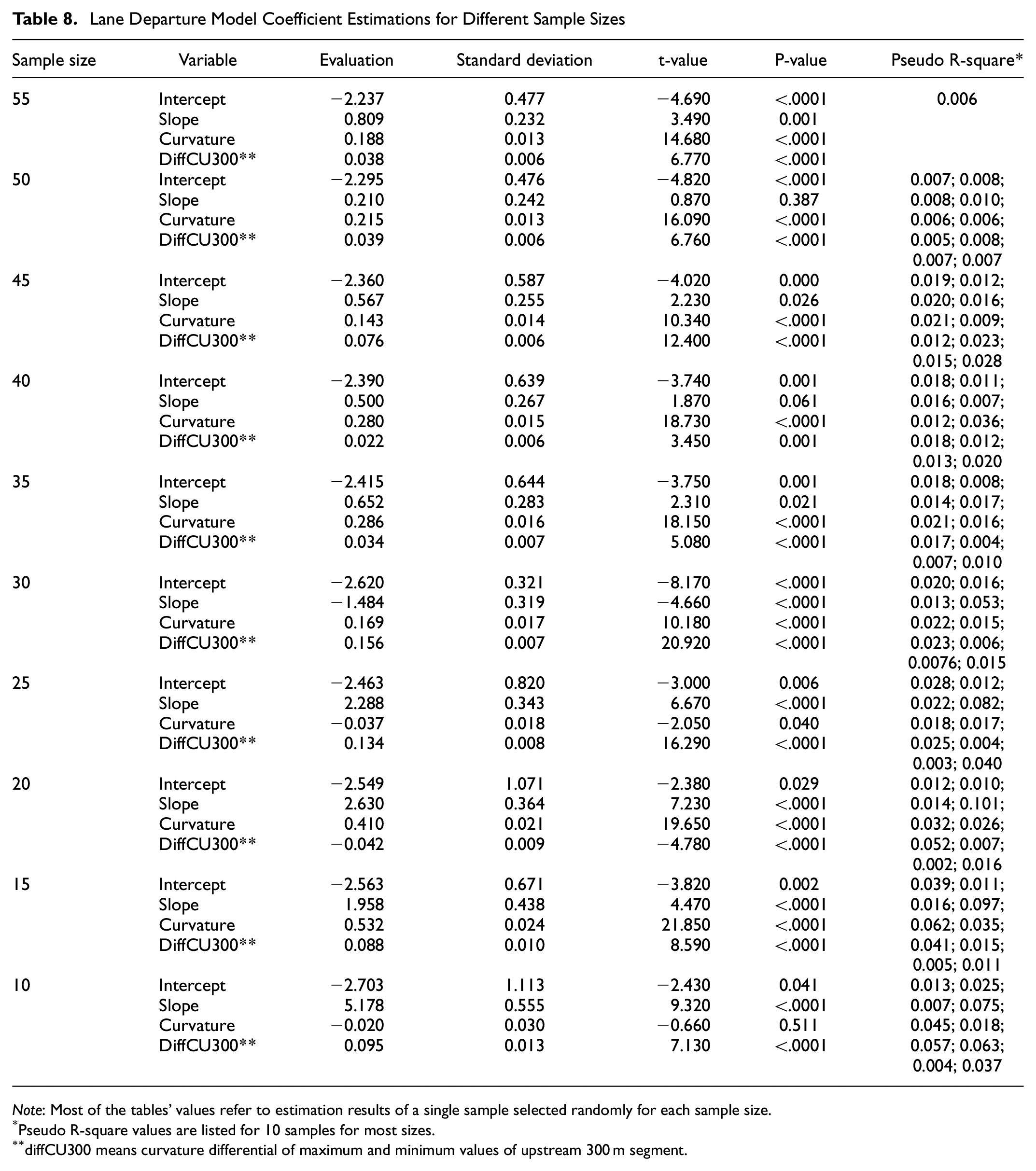
Note: Most of the tables’ values refer to estimation results of a single sample selected randomly for each sample size.

Pseudo R-square values are listed for 10 samples for most sizes.

diffCU300 means curvature differential of maximum and minimum values of upstream 300 m segment.

The significance of the intercept implies that the existence of individual discrepancies is substantially related to lane departure; consequently, drivers’ individual effects cannot be neglected. Pseudo R-square values for the 10 generated samples of each size are listed in Table 8, where they can be seen to fluctuate between 0.006 and 0.188 for sample sizes less than 25. The change of pseudo R-square stabilizes as the sample size becomes larger than 30, indicating the models have become more trustworthy.

Coefficients of intercept, slope, curvature, and diffCU300 were calculated by the random sampling method of selecting 5 drivers for every increased sample step 10 times. Boxplots were constructed to check the converging stability of each variable in the different sample sizes, where variability is measured by interquartile, and the bands inside the boxes are the medians (Figure 8).

Figure 8.

Box-plot of lane departure model coefficient estimation of different sample sizes: (a) intercept, (b) slope, (c) curvature, and (d) diffCU300.

The general trend of the four variables is that as sample size increased, fluctuations of estimated coefficients tended to decrease. Stability can be inferred from the gradual attenuated fluctuation of the parameter coefficients. Median and variability are good measures of fluctuations with change of sample size, so stability is implied in the change of interquartile range becoming stable after a certain sample size is reached. As seen in Figure 8, some variables reached stability quickly as sample size increased, but others are less sensitive to the increase. Slope converged at around 20, for example, but stability for curvature and diffCU300 was achieved at a sample size of around 30.

As with the speed model, however, determination of acceptable sample size requires mathematical validation using quantitative measurement methods such as MSE rather than relying on subjective approaches. Figure 9 depicts the change in MSE as lane departure sample size increased.

Figure 9.

Mean squared error (MSE) of each variable for different lane departure sample sizes: (a) intercept, (b) slope, (c) curvature, and (d) diffCU300.

Convergence patterns for the different variables can be seen to be similar. All variables converged quickly in response to the increase in sample size. Slope converged when the sample size reached 25, and curvature and diffCU300 patterns converged at 35. The converged point is the tipping point to indicate that patterns remain the same after the tipping point.

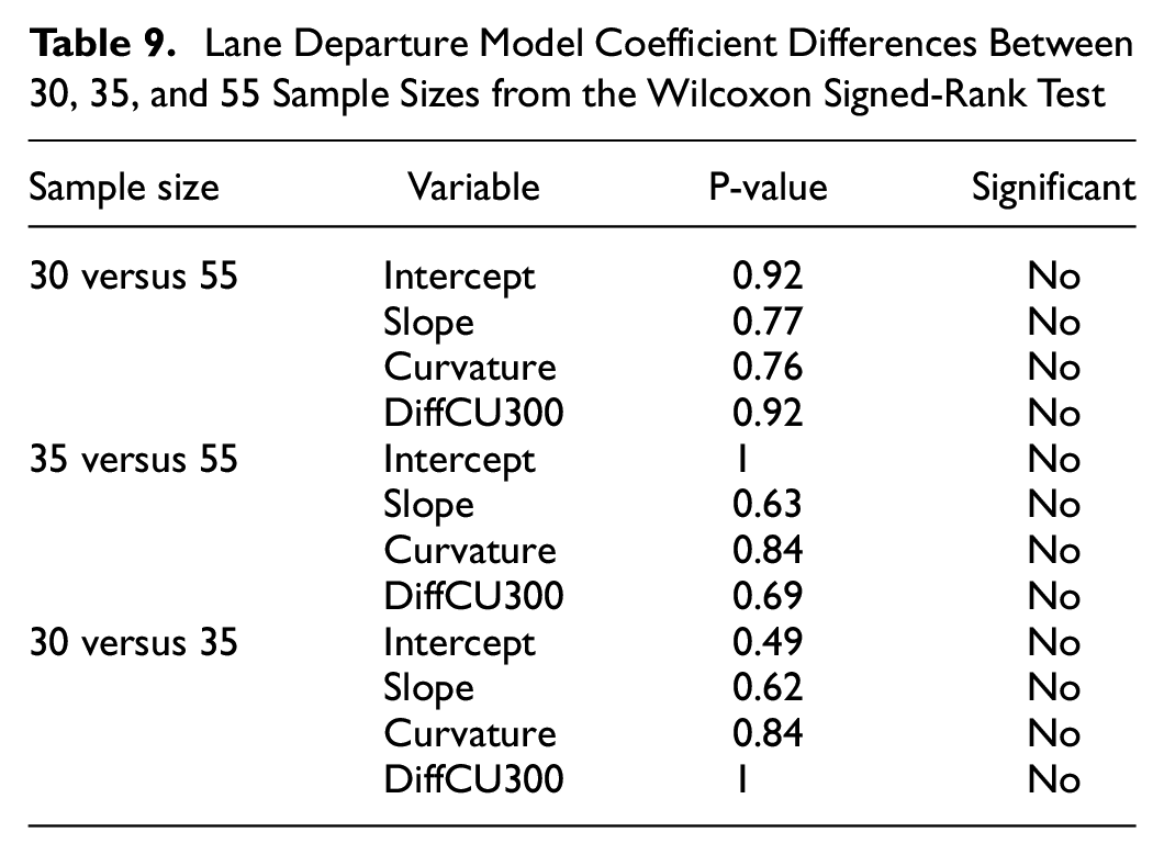
As evidenced from the boxplots and MSE curves, sample sizes of both 30 and 35 appear to be acceptable for lane departure, so the Wilcoxon signed-rank test was used to determine whether the coefficients of the 25-driver sample, the 30-driver sample, and the 35-driver sample are significantly different from those of the full-size 55-driver model. The Wilcoxon signed-rank test was also conducted to compare the difference between the 30 and 35 model sizes.

Because 55 is used as the full sample size in this paper, the bigger the sample size (closer to 55), the smaller the difference compared with 55 sample size. If smaller sample size is converged, then larger sample size is expected to be converged as well.

Differences between these two models were assessed by the Wilcoxon signed-rank test. Insignificance of variable indicates that no difference was detected on this certain variable in two models with respective sample sizes. As shown in Table 9, compared with the full-size model, the model of sample size 30 and the model of sample size 35 do not appear significantly different, since all regressed variables were insignificant. It is appropriate to choose both sample sizes of 30 and 35 in the mixed logistic regression model of lane departure to replace the full-size model of 55 drivers. The smaller the sample, the bigger the difference will be compared with the population (i.e., 55). Since 30 sample size is just starting to converge, 25 or 20 sample size is, by definition, not yet converged.

Table 9.

Lane Departure Model Coefficient Differences Between 30, 35, and 55 Sample Sizes from the Wilcoxon Signed-Rank Test

Sample size	Variable	P-value	Significant
30 versus 55	Intercept	0.92	No
	Slope	0.77	No
	Curvature	0.76	No
	DiffCU300	0.92	No
35 versus 55	Intercept	1	No
	Slope	0.63	No
	Curvature	0.84	No
	DiffCU300	0.69	No
30 versus 35	Intercept	0.49	No
	Slope	0.62	No
	Curvature	0.84	No
	DiffCU300	1	No

Therefore, a sample size of 30 drivers should be sufficient for building a mixed linear regression speed model for the parsimonious rule of cost saving.

Discussion and Conclusion

This study proposes a way to determine acceptable sample size, and offers a recommendation for future sample sizes related to modeling techniques and performance measures. The paper takes into consideration two general conditions in the driving simulator study of geometric design safety evaluation. The mixed linear regression model was used to establish the relationship between geometric design features and vehicle speed. The mixed logistic regression model was used to establish the relationship between geometric design features and lane departure. An empirical method of choosing acceptable sample size was executed by checking the convergence, measured by MSEs, of selected variables in the mixed effects models. Thirty was determined to be the proper number to be selected as the acceptable sample size in our study.

The method of determining acceptable sample size depending on the elbow of the models’ estimated coefficients is an approach analogous to the elbow method in unsupervised learning cluster analysis, which provides a way to choose the number of clusters based on convergence of the computed sum of squared error for certain values of the number of clusters ( 53 ). The elbow method is a classical method for cluster analysis that validates the acceptable number of clusters in situations where the loss function is unknown and pre-assumptions cannot be specified. A similar idea to the Elbow method is initiated in this paper—a steady trend referring to the MSE, which avoids the difficulty of finding loss function and inventing assumptions about geometric design features ( 10 ). Random sampling was used in this research. A relatively homogeneous subject sample was selected for this study to avoid biased results caused by irrelevant factors. This homogeneity is common in driving simulator studies, as it permits a sample smaller than that which would be needed for a more heterogenous sample. Generally, the more characteristics taken into consideration, the larger the required sample size. The acceptable experimental sample size found in this study, then, was applicable to the effects of roadway geometric characteristics of combined alignments on speed and lane departure, and the particular driving characteristics of a homogenous sample ( 42 ). Results should, therefore, not be understood as absolute values for driving simulator research of roadway design safety evaluation.

This method to determine the sample size by convergence of the models’ estimated coefficients can not only be applied in road design safety assessment, but can also be taken advantage of in experiments with homogeneous samples with specific evaluation indicators. Thirty can be utilized as an acceptable sample size in road safety assessments on mountainous freeways because the road conditions and metrics used in driving simulation experiments are close. If road environment and traffic scenarios, such as urban or rural road scenarios, in driving simulator experiments differ too much from the mountain freeways that are used as an example in this paper, then 30 may not be used directly as the least acceptable sample size. For other distinct road conditions, driving simulation experiments can be devised to identify the acceptable sample size using the method described in this paper.

Supplemental Material

sj-docx-1-trr-10.1177_03611981221144296 – Supplemental material for Sample Size Study of Driving Simulator Experiment for Freeway Design Safety Evaluations

Supplemental material, sj-docx-1-trr-10.1177_03611981221144296 for Sample Size Study of Driving Simulator Experiment for Freeway Design Safety Evaluations by Xuesong Wang, Shuang Liu, Bowen Cai, David Hurwitz, Qiming Guo and Xiaomeng Wang in Transportation Research Record

Footnotes

Author Contributions

The authors confirm contribution to the paper as follows: study conception and design: X. Wang, S. Liu, B. Cai, D. Hurwitz, Q. Guo; data collection: X. Wang, S. Liu, B. Cai, D. Hurwitz, Q. Guo; analysis and interpretation of results: X. Wang, S. Liu, B. Cai, D. Hurwitz, Q. Guo; draft manuscript preparation: X. Wang, S. Liu, B. Cai, D. Hurwitz, Q. Guo. All authors reviewed the results and approved the final version of the manuscript.

Declaration of Conflicting Interests

The author(s) declared no potential conflicts of interest with respect to the research, authorship, and/or publication of this article.

Funding

The author(s) disclosed receipt of the following financial support for the research, authorship, and/or publication of this article: This work was supported by the Chinese National Science Foundation (51878498), and the Driving Simulation Research Project of Shuilang Interchange on Shenzhen Jihe Freeway.

Compliance with Ethics Guidelines

The study was approved by the Ethics Committee of Tongji University.

Data Accessibility Statement

When conducting the driving simulator experiment, informed consent form (ICF) templates were signed with participants, clearly stating that the data of the participants collected in the experiment was only used within the research team, to protect the participants’ privacy. Therefore, according to the agreement of ICF templates, the authors cannot share the data of this paper.

Supplemental Material

Supplemental material for this article is available online.

ORCID iDs

Xuesong Wang

Bowen Cai

David Hurwitz

References

Keith

Trentacoste

M. F.

Depue

Granda

T. M.

Huckaby

Ibarguen

Kantowitz

B. H.

Lum

Wilson

Roadway Human Factors and Behavioral Safety in Europe. Tech Report. FHWA-PL-05-005. Federal Highway Administration, Washington D.C., 2005.

Fisher

D. L.

Caird

J. K.

Rizzo

Lee

J. D.

Handbook of Driving Simulation for Engineering, Medicine and Psychology: An Overview. In Handbook of Driving Simulation for Engineering, Medicine, and Psychology ( Fisher

D. L.

Rizzo

Caird

Lee

J. D.

, eds.), CRC Press, Boca Raton, FL, 2011, pp. 1-1–1-16.

Shinar

Traffic Safety and Human Behavior. Emerald Publishing Limited, Bingley, 2017.

Ministry of Transportation of the People’s Republic of China. Specification for Highway Safety Audit: JTG B05-2015. China Communication Press, Beijing, 2016.

Bella

Driver Perception of Roadside Configurations on Two-Lane Rural Roads: Effects on Speed and Lateral Placement. Accident Analysis & Prevention, Vol. 50, 2013, pp. 251–262.

Bella

Driver Performance Approaching and Departing Curves: Driving Simulator Study. Traffic Injury Prevention, Vol. 15, No. 3, 2014, pp. 310–318. https://doi.org/10.1080/15389588.2013.813022.

Bella

Operating Speeds from Driving Simulator Tests for Road Safety Evaluation. Journal of Transportation Safety and Security, Vol. 6, No. 3, 2014, pp. 220–234. https://doi.org/10.1080/19439962.2013.856984.

Bella

Driving Simulator for Speed Research on Two-Lane Rural Roads. Accident Analysis & Prevention, Vol. 40, No. 3, 2008, pp. 1078–1087. https://doi.org/10.1016/j.aap.2007.10.015.

Aguirre-Urreta

Rönkkö

Sample Size Determination and Statistical Power Analysis in PLS Using R: An Annotated Tutorial. Communications of the Association for Information Systems, Vol. 36, No. 1, 2015, p. 3.

10.

Bausell

R. B.

Power Analysis for Experimental Research: A Practical Guide for the Biological, Medical, and Social Sciences. Cambridge University Press, New York, 2002.

11.

Festing

M. F. W.

On Determining Sample Size in Experiments Involving Laboratory Animals. Laboratory Animals, Vol. 52, No. 4, 2018, pp. 341–350.

12.

Singh

A. S.

Masuku

M. B.

Sampling Techniques & Determination of Sample Size in Applied Statistics Research: An Overview. International Journal of Economics, Commerce and Management, Vol. 2, No. 11, 2014, pp. 1–22.

13.

Cox

D. R.

Reid

The Theory of the Design of Experiments. Chapman and Hall/CRC Press, Boca Raton, FL, 2000.

14.

Zhao

Chen

Rong

Modeling the Influence of Chevron Alignment Sign on Young Male Driver Performance: A Driving Simulator Study. Accident Analysis & Prevention, Vol. 95, 2016, pp. 479–486. https://doi.org/10.1016/j.aap.2016.04.024.

15.

Ben-Bassat

Shinar

Effect of Shoulder Width, Guardrail and Roadway Geometry on Driver Perception and Behavior. Accident Analysis & Prevention, Vol. 43, No. 6, 2011, pp. 2142–2152.

16.

van der Horst

de Ridder

Influence of Roadside Infrastructure on Driving Behavior: Driving Simulator Study. Transportation Research Record: Journal of the Transportation Research Board, 2007. 2018: 36–44.

17.

Calvi

Benedetto

de Blasiis

M. R.

A Driving Simulator Study of Driver Performance on Deceleration Lanes. Accident Analysis & Prevention, Vol. 45, 2012, pp. 195–203. https://doi.org/10.1016/j.aap.2011.06.010.

18.

Mead

The Design of Experiments: Statistical Principles for Practical Applications. Cambridge University Press, 1990.

19.

Ding

Zhao

Rong

Experimental Research on the Effectiveness of Speed Reduction Markings Based on Driving Simulation: A Case Study. Accident Analysis & Prevention, Vol. 60, 2013, pp. 211–218. https://doi.org/10.1016/j.aap.2013.08.007.

20.

Cohen

Statistical Power Analysis for the Behavioral Sciences. Routledge, New York, NY, 2013.

21.

Chen

D.-G.

Fraser

M. W.

A Bayesian Approach to Sample Size Estimation and the Decision to Continue Program Development in Intervention Research. Journal of the Society for Social Work and Research, Vol. 8, No. 3, 2017, pp. 457–470.

22.

Lamm

Psarianos

Mailaender

Highway Design and Traffic Safety Engineering Handbook. McGraw-Hill, New York, NY, 1999.

23.

Hancock

M. W.

Wright

A Policy on Geometric Design of Highways and Streets. American Association of State Highway and Transportation Officials, Washington, DC, 2018.

24.

Horberry

Anderson

Regan

M. A.

The Possible Safety Benefits of Enhanced Road Markings: A Driving Simulator Evaluation. Transportation Research Part F: Traffic Psychology and Behaviour, Vol. 9, No. 1, 2006, pp. 77–87. https://doi.org/10.1016/j.trf.2005.09.002.

25.

Chrysler

T. S.

Williams

Driving Performance in a Simulator as a Function of Pavement and Shoulder Width, Edge Line Presence, and Oncoming Traffic. Proc., Driving Assessment 2005: 3rd International Driving Symposium on Human Factors in Driver Assessment, Training, and Vehicle Design, Rockport, ME, University of Iowa, June 27–30, 2005, 6p.

26.

Bella

Operating Speed Predicting Models on Two-Lane Rural Roads From Driving Simulation. Presented at 84th Annual Meeting of the Transportation Research Board, Washington, D.C., 2005.

27.

Daniels

Vanrie

Dreesen

Brijs

Additional Road Markings as an Indication of Speed Limits: Results of a Field Experiment and a Driving Simulator Study. Accident Analysis & Prevention, Vol. 42, No. 3, 2010, pp. 953–960. https://doi.org/10.1016/j.aap.2009.06.020.

28.

García

Dols

Moreno

A. T.

Tarko

Calatayud

Analysis of the Influence of 3D Coordination on the Perception of Horizontal Curvature Using Driving Simulator. Advances in Transportation Studies an International Journal, Vol. 24, 2011, pp. 33–44.

29.

Montella

Aria

D’Ambrosio

Galante

Mauriello

Pernetti

Simulator Evaluation of Drivers’ Speed, Deceleration and Lateral Position at Rural Intersections in Relation to Different Perceptual Cues. Accident Analysis & Prevention, Vol. 43, No. 6, 2011, pp. 2072–2084.

30.

Zhang

The Impact of Driving Speed on Driving Track on Low-Grade Highways in Mountain Area. Journal of Transport Science and Engineering, Vol. 28, 2012, pp. 59–64.

31.

Yang

Overton

Han

L. D.

Yan

Richards

S. H.

The Influence of Curbs on Driver Behaviors in Four-Lane Rural Highways – A Driving Simulator Based Study. Accident Analysis & Prevention, Vol. 50, 2013, pp. 1289–1297. https://doi.org/10.1016/j.aap.2012.09.031.

32.

Calvi

D’Amico

A Study of the Effects of Road Tunnel on Driver Behavior and Road Safety Using Driving Simulator. Advances in Transportation Studies, Vol. 30, 2013, pp. 59–76.

33.

Wang

Lin

Yang

Evaluating Alignment Consistency for Mountainous Expressway in Design Stage: A Driving Simulator-Based Approach. Presented at 92th Annual Meeting of the Transportation Research Board, Washington, D.C., 2013.

34.

Calvi

Bella

Modeling Speed Differential Parameters in Day and Night Environments Using Driving Simulator. Procedia Engineering, Vol. 84, 2014, pp. 648–661. https://doi.org/10.1016/j.proeng.2014.10.482.

35.

Bella

Calvi

D’Amico

Analysis of Driver Speeds Under Night Driving Conditions Using a Driving Simulator. Journal of Safety Research, Vol. 49, 2014, pp. 45–52. https://doi.org/10.1016/j.jsr.2014.02.007.

36.

Bella

Coordination of Horizontal and Sag Vertical Curves on Two-Lane Rural Roads: Driving Simulator Study. IATSS Research, Vol. 39, No. 1, 2015, pp. 51–57. https://doi.org/10.1016/j.iatssr.2015.02.002.

37.

Wang

Tarko

Tremont

P. J.

The Influence of Combined Alignments on Lateral Acceleration on Mountainous Freeways: A Driving Simulator Study. Accident Analysis & Prevention, Vol. 76, 2015, pp. 110–117. https://doi.org/10.1016/j.aap.2015.01.003.

38.

Domenichini

la Torre

Branzi

Nocentini

Speed Behaviour in Work Zone Crossovers. A Driving Simulator Study. Accident Analysis & Prevention, Vol. 98, 2017, pp. 10–24. https://doi.org/10.1016/j.aap.2016.09.018.

39.

Bella

Silvestri

Interaction Driver–Bicyclist on Rural Roads: Effects of Cross-Sections and Road Geometric Elements. Accident Analysis & Prevention, Vol. 102, 2017, pp. 191–201.

40.

Filtness

A. J.

Larue

Schramm

Fuller

Rakotonirainy

Han

Cairney

Safety Implications of Co-Locating Road Signs: A Driving Simulator Investigation. Transportation Research Part F: Traffic Psychology and Behaviour, Vol. 47, 2017, pp. 187–198.

41.

Beanland

Grant

Read

G. J. M.

Stevens

Thomas

Lenné

M. G.

Stanton

N. A.

Salmon

P. M.

Challenging Conventional Rural Rail Level Crossing Design: Evaluating Three New Systems Thinking-Based Designs in a Driving Simulator. Safety Science, Vol. 110, 2018, pp. 100–114. https://doi.org/10.1016/j.ssci.2018.03.002.

42.

Chen

Quddus

Wang

Impact of Combined Alignments on Lane Departure: A Simulator Study for Mountainous Freeways. Transportation Research Part C: Emerging Technologies, Vol. 86, 2018, pp. 346–359. https://doi.org/10.1016/J.TRC.2017.11.010.

43.

Charlton

S. G.

Starkey

N. J.

Malhotra

Using Road Markings as a Continuous Cue for Speed Choice. Accident Analysis & Prevention, Vol. 117, 2018, pp. 288–297. https://doi.org/10.1016/j.aap.2018.04.029.

44.

Wang

Speed Change Behavior on Combined Horizontal and Vertical Curves: Driving Simulator-Based Analysis. Accident Analysis & Prevention, Vol. 119, 2018, pp. 215–224.

45.

Wang

Cai

Liu

Combined Alignment Effects on Deceleration and Acceleration: A Driving Simulator Study. Transportation Research Part C: Emerging Technologies, Vol. 104, 2019, pp. 172–183. https://doi.org/10.1016/j.trc.2019.04.027.

46.

Kazemzadehazad

Monajjem

Larue

G. S.

King

M. J.

Evaluating New Treatments for Improving Driver Performance on Combined Horizontal and Crest Vertical Curves on Two-Lane Rural Roads: A Driving Simulator Study. Transportation Research Part F: Traffic Psychology and Behaviour, Vol. 62, 2019, pp. 727–739. https://doi.org/10.1016/j.trf.2019.03.002.

47.

Bassani

Catani

Salussolia

Yang

C. Y. D.

A Driving Simulation Study to Examine the Impact of Available Sight Distance on Driver Behavior Along Rural Highways. Accident Analysis & Prevention, Vol. 131, 2019, pp. 200–212. https://doi.org/10.1016/j.aap.2019.07.003.

48.

Wang

Chen

Guo

Tarko

Lizarazo

Wang

Transferability Analysis of the Freeway Continuous Speed Model. Accident Analysis & Prevention, Vol. 151, 2021, p. 105944.

49.

National Academies of Sciences, Engineering, and Medicine. Evaluation of Data Needs, Crash Surrogates, and Analysis Methods to Address Lane Departure Research Questions Using Naturalistic Driving Study Data. The National Academies Press, Washington, D.C., 2011. https://doi.org/10.17226/22848.

50.

Torbic

D. J.

Harwood

D. W.

Gilmore

D. K.

Pfefer

Neuman

T. R.

Slack

K. L.

Hardy

K. K.

Guidance for Implementation of the AASHTO Strategic Highway Safety Plan. Transportation Research Board, Washington, D.C., 2004.

51.

Profession Standard of the People’s Republic of China. Design Specification for Highway Alignment: JTG D20-2017. People’s Communications Press, Beijing, 2017.

52.

Strano

Colosimo

B. M.

Logistic Regression Analysis for Experimental Determination of Forming Limit Diagrams. International Journal of Machine Tools and Manufacture, Vol. 46, No. 6, 2006, pp. 673–682.

53.

Tibshirani

Walther

Hastie

Estimating the Number of Clusters in a Data Set via the Gap Statistic. Journal of the Royal Statistical Society: Series B (Statistical Methodology), Vol. 63, No. 2, 2001, pp. 411–423.

54.

Wilcoxon

Individual Comparisons by Ranking Methods. In Breakthroughs in Statistics ( Kotz

Johnson

N. L.

, eds.), Springer, New York, NY, 1992, pp. 196–202.

55.

Xia

Correlation and Association Analyses in Microbiome Study Integrating Multiomics in Health and Disease. Progress in Molecular Biology and Translational Science, Vol. 171, 2020, pp. 309–491.

56.

Nakagawa

Schielzeth

A General and Simple Method for Obtaining R2 From Generalized Linear Mixed-Effects Models. Methods in Ecology and Evolution, Vol. 4, No. 2, 2013, pp. 133–142. https://doi.org/10.1111/j.2041-210x.2012.00261.x.

Supplementary Material

Please find the following supplemental material available below.

For Open Access articles published under a Creative Commons License, all supplemental material carries the same license as the article it is associated with.

For non-Open Access articles published, all supplemental material carries a non-exclusive license, and permission requests for re-use of supplemental material or any part of supplemental material shall be sent directly to the copyright owner as specified in the copyright notice associated with the article.

0.00 MB

0.03 MB