Modeling Exhaust-Generated Aerodynamic Pressure Loads on Airfield Matting Repair Systems

Abstract

Airfield matting systems are commonly used for rapid repair of damaged runways to facilitate continuity of critical operations. Under normal service conditions, matting repair systems are subject not only to wheel loads exerted by airfield traffic but also to aerodynamic pressure loads resulting from high-speed, turbulent exhaust plumes produced by jets during taxi and take-off. Matting systems employed by the U.S. Air Force have been tested with respect to wheel loads, but probabilities of failure because of pressure loads produced by jet exhaust have not yet been established. This study presents a numerical approach for preliminary estimation of worst-case matting anchor forces resulting from exhaust-generated pressure loads. Using a two-dimensional computational fluid dynamics model, system behavior is evaluated by means of a parametric study of six system variables, of which the most significant are: (1) distance between engine and matting, (2) depth of cavity openings at matting edges, and (3) engine exhaust velocity. The results demonstrate that matting systems are likely to experience net uplift in typical service scenarios, driven by the combined effects of flow separation and cavity pressurization. Worst-case anchor pull-out forces, computed according to a tributary-area approach, are estimated to fall in the range of 130 lb (581 N) to 979 lb (4,350 N), depending on assumed load-sharing behavior among anchors and the size of the repair site. Field testing of instrumented matting systems during jet taxi and take-off sequences is recommended as the best next step toward understanding system behavior.

Keywords

aviation aircraft/airport compatibility airport pavement airport safety operations

Airfields are a crucial part of military infrastructure. Interruption of airfield operations by a bomb strike or debris impacts that deform an airstrip may severely constrain the fleet it serves, rendering planes on the ground useless and leaving those in the air without a safe place to land. This recognized vulnerability has spurred the development of airfield damage repair (ADR) procedures to restore an even pavement surface and resume operations in a matter of minutes. One standard ADR method employed by the U.S. Air Force (USAF) involves first leveling the repair site by back-filling the crater with crushed stone and other aggregate material and mechanically compacting it ( 1 ). A foreign-object debris (FOD) cover, consisting of fiber composite matting, is then assembled and placed over the repair site and secured to the undamaged pavement by anchor bolts, recreating a smooth, durable surface suitable for landing and take-off traffic. The matting systems used for this purpose by the USAF have been tested with respect to wheel loads exerted by airfield traffic and were found to have adequate strength to meet these demands ( 1 ).

Another potential source of damage, which has not yet been specifically addressed in any study, is the aerodynamic loading produced by upstream jet engine exhaust plumes. If the uplift pressures developed on a matting system by a worst-case turbulent exhaust impact are severe enough to reach a reasonably high probability of system failure, pressure-reduction measures or redesigned connections may be warranted, but no test data or simulation results have been made available to this point to characterize the expected load intensity. This paper presents the findings of a numerical investigation of exhaust-generated pressure loads on airfield matting systems, specifically ADR systems used by the USAF. The objective of the study is to offer a first estimate of pressure load intensities and consequent worst-case anchor pull-out forces that can be expected under typical service conditions.

Airfield Matting Repair Systems

This study considers two classes of matting used by the USAF as FOD covers: folded fiberglass matting (FFM) and fiber-reinforced polymer (FRP) matting. FFM was the standard USAF matting solution for some decades; though these systems were serviceable for the heaviest craft operating in the USAF fleet before 1990, field testing performed in 2005 found FFM panels insufficiently resistant to C-17 wheel traffic loads ( 1 ). These same tests also evaluated a legacy FRP matting system and found it inadequate for expected traffic loads because of connector and anchor bushing failures. The current FRP matting system was developed out of the legacy system with redesigned connections. The ADR manual maintained by the Tri-Service Pavements Working Group, last updated in 2020, which guides airfield repair operations for the USAF as well as the U.S. Army and U.S. Navy, provides documentation and installation instructions for both FFM and FRP matting ( 2 ).

FFM units are composed of nine individual fiberglass panels measuring 6 ft by 30 ft (1.83 m by 9.14 m) in area and 0.5 in. (12.7 mm) in thickness. Panels are connected by elastomer hinges 3 in. (76.2 mm) in width that permit the panels to be folded for storage and transport. The approximate weight of a single nine-panel FFM unit is 3,000 lb (1,360 kg) ( 2 ). Anchor holes are spaced at 2 ft (0.609 m) along the perimeter of the FFM to facilitate anchorage. FFM installation is pictured in Figure 1. A single FFM unit, suitable for repair of craters up to 28 ft (8.53 m) in diameter, is depicted in plan view in Figure 2. For larger repairs, FFM units may be spliced together.

Figure 1.

Folded fiberglass matting (FFM) systems installed during airfield damage repair (ADR) exercises at Osan Air Base, Republic of Korea.

Figure 2.

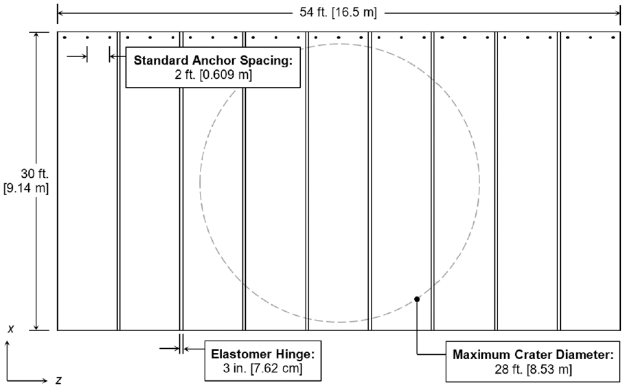
Typical folded fiberglass matting (FFM) system for a small- or medium-scale pavement repair. Anchors are shown on one edge only but are present along the entire perimeter. Airfield traffic travels in the x direction.

FRP matting systems are more modular in form than FFM units. FRP systems are assembled from full panels, measuring 6.67 ft (2.03 m) in width by 18 ft (5.49 m) in length, and half panels, equal in width to full panels but 9 ft (2.74 m) in length. FRP panels have a standard thickness of 0.5 in. (12.7 mm). The ADR manual published by the Pavements Working Group does not include a weight estimate for FRP matting as it does for FFM; if the polymer composite used in FRP matting is assumed to have a density comparable to that of the fiberglass used in FFM, the unit weight of FRP matting is approximately 1.85 lb/ft² (9.03 kg/m²). Anchor holes are spaced at 2 ft (0.609 m) along the edges of each panel for anchorage to the pavement and for inter-panel connections. This spacing is typical for most of the perimeter of each panel, though holes are spaced more closely at panel corners and at the center of the long dimension of full panels. FRP matting installation is pictured in Figure 3. Example FRP matting assemblies for a small-scale repair, composed of one full panel and two half panels, and a medium-scale repair, consisting of two full panels and two half panels, are depicted in Figure 4. Matting assemblies for larger repair sites are constructed similarly, with panels arranged in staggered fashion.

Figure 3.

Fiber-reinforced polymer (FRP) matting system installed over a simulated large-scale repair site during field tests at Tyndall Air Force Base, Florida.

Figure 4.

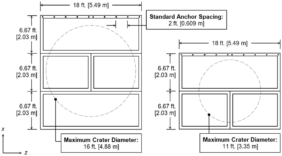
Typical fiber-reinforced polymer (FRP) matting assemblies for medium- and small-scale pavement repairs. Anchors are shown on one edge only but are present along the entire perimeter. Airfield traffic travels in the x direction.

Aerodynamic Loading Mechanisms

Engine exhaust plumes have been an important topic of research to the aerospace community for at least the past 50 years. Before the advent of gas turbine engines, the wake generated by propeller-driven planes during taxi and take-off—commonly called “prop-wash”—was never a substantial threat to life or property but, as commercial and military aviation transitioned to jet-engine-powered craft, the high-velocity, turbulent exhaust plumes produced by these jets quickly signaled a need to address safety issues and implement damage mitigation measures on airfields, in relation to structure frangibility and other non-fixed structures such as noise mitigation panels and specific pavement repairs ( 5 ). In the case of airfield matting systems, the probable controlling limit state because of exhaust plume interaction is that of anchor pull-out failure as a consequence of matting uplift. For pull-out failure to occur, the plume must generate a net uplift pressure load across the matting sufficient to overcome the vertical pull-out resistance of the critical anchor in the system. Three loading mechanisms conducive to the development of net uplift pressures are: flow separation, cavity pressurization, and the formation of spatio-temporal pressure gradients.

Boundary-layer flow refers to the local flow field that forms around an object immersed in a moving fluid ( 6 , 7 ). In the case of a blunt object, as fluid flow travels around the leading edge of the object, a region of flow separation forms as depicted in Figure 5a. In this illustration, exhaust-generated airflow approaches the leading edge of the matting system. Rapid acceleration of airflow around the edge of the matting produces a local region of recirculation as the flow separates from the matting surface before reattaching at some length downstream of the leading edge. The reattachment length is a function of the local Reynolds number, upstream turbulence intensity, and object geometry, among other variables ( 8 , 9 ). Within the flow separation region, the gauge static pressure on the top surface of the matting is negative—that is, the local static pressure is below atmospheric pressure. On the bottom surface, the gauge static pressure is closer to zero. The resulting pressure differential tends to lift the matting in this region.

Figure 5.

Expected flow behavior at the upstream edge of a typical matting system, including (a) flow separation and (b) cavity pressurization.

The presence of a cavity beneath an object immersed in a fluid provides another mechanism for uplift. Numerous studies have demonstrated that cavity flow is characteristically laminar, with a nearly uniform cavity pressure that is largely a function of cavity depth, the width of cavity openings, and the flow velocity at the cavity entrance ( 10 – 12 ). In cases where the local flow field develops a positive gauge static pressure in the cavity, the result is an uplift force on the bottom surface of the object. The loading mechanism of cavity pressurization is illustrated in Figure 5b, which depicts the portion of the cavity near the upstream edge of the matting system. Exhaust approaching the cavity opening rapidly slows down as it enters the cavity; the loss of dynamic pressure drives a rise in static pressure such that a nearly uniform positive static pressure, represented by the darkest contour in Figure 5b, is attained throughout the whole cavity length, except near the upstream and downstream edge regions.

Closely related to the mechanism of cavity pressurization is the formation of spatio-temporal pressure gradients. Turbulent, free-stream flow above the matting is attended by rapid pressure fluctuations along the top surface produced by separating and reattaching flow, in contrast to the laminar flow below the matting with its more stable, uniform pressure ( 13 – 15 ). As a consequence, sharp pressure gradients tend to develop that vary in space and time. The contribution of this loading mechanism to matting uplift is potentially very significant, especially in cases where the exhaust plume completely envelopes the matting, since this state combines intense turbulent flow on the top surface with positive cavity pressures on the bottom surface. Since time-averaged simulations, which are employed in this study, conceal the impact of spatio-temporal effects, neglecting the influence of this mechanism contributes to underestimation of net forces in the results presented hereafter.

Methods

Computational fluid dynamics (CFD) modeling has become an essential component of aerospace research and development ( 16 ). Past studies have applied CFD approaches to investigate aerodynamic and aeroacoustic effects in the near-downstream region of engine exhaust systems ( 17 , 18 ). Others have developed CFD models of engine exhaust wake to guide the design of components in jet engine test facilities and evaluate the performance of jet-blast deflector systems on airfields, though the aerodynamic loading of airfield matting systems by engine exhaust has not yet been addressed ( 19 , 20 ).

Fluid motion is governed by the Navier–Stokes equations, which consist of a set of coupled equations that enforce conservation of mass and momentum in a fluid domain ( 21 ). Because they cannot be solved analytically except in the simplest cases, CFD methods have been developed to solve the Navier–Stokes equations numerically. The three broad categories of Navier–Stokes analysis methods are: (1) direct numerical simulation (DNS), which solves the governing equations down to the smallest scale of interest without numerical approximation; (2) large-eddy simulation (LES), in which a filter is applied to the governing equations such that turbulent fluctuations above the cutoff scale are resolved and those below are treated with a model; and (3) Reynolds-averaged Navier–Stokes (RANS) methods, in which the flow variables in the governing equations are time-averaged and turbulence at all scales is described by a turbulence model ( 22 ). Of these categories of methods, DNS affords the highest solution accuracy, but the high computational demands of DNS approaches limit its use to problems involving low Reynolds number flows and idealized geometries ( 23 ). RANS methods are limited in their ability to capture turbulent effects and thus provide a lower order of accuracy than either DNS or LES, but the substantially higher computational efficiency offered by RANS accounts for its common use in turbulent flow studies, including jet engine performance studies ( 24 ). LES methods fall between DNS and RANS in accuracy and computational demand. While the superior accuracy of LES in studies of engine exhaust plumes has been established, it has nevertheless been suggested that RANS methods may yield approximate results that are adequate for the purposes of preliminary design or analysis ( 17 , 23 ). On this view, a RANS method is employed in this study to obtain a first estimate of exhaust-generated flow fields and the resulting forces acting on matting systems.

Governing Equations

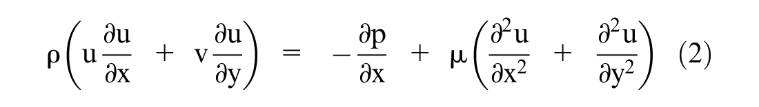
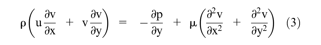
For a two-dimensional domain, the Navier–Stokes equations for continuity and momentum may be expressed as in Equations 1–3:

\frac{\partial u}{\partial x} + \frac{\partial v}{\partial y} = 0

(1)

ρ (u \frac{\partial u}{\partial x} + v \frac{\partial u}{\partial y}) = - \frac{\partial p}{\partial x} + μ (\frac{\partial^{2} u}{\partial x^{2}} + \frac{\partial^{2} u}{\partial y^{2}})

(2)

ρ (u \frac{\partial v}{\partial x} + v \frac{\partial v}{\partial y}) = - \frac{\partial p}{\partial y} + μ (\frac{\partial^{2} v}{\partial x^{2}} + \frac{\partial^{2} v}{\partial y^{2}})

(3)

where

u = fluid velocity component in the x direction,

v = fluid velocity component in the y direction,

ρ = fluid density,

μ = fluid dynamic viscosity, and

p = static pressure.

This form of the Navier–Stokes equations is time-averaged and assumes incompressible flow and negligible gravitational and thermal effects. Though this analysis considers exhaust velocities for which Ma > 0.30 in the near-downstream region of the engine exit nozzle, the incompressibility assumption is made since Ma < 0.30 everywhere in the local flow field around the affected matting system, which is the region of interest to this study.

In addition to the RANS equations of motion defined in Equations 1–3, a turbulence model is needed to provide a complete set of coupled equations. Recognizing that past turbulent jet studies have commonly used some form of the two-equation k-ε or k-ω turbulence model, the realizable k-ε model is selected for the present analysis ( 25 – 27 ). The model consists of two transport equations for variables k and ε, which represent the turbulent kinetic energy and the turbulent dissipation rate, respectively. The transport equations are given in Equations 4 and 5:

\begin{matrix} \frac{\partial}{\partial t} (ρ k) + \frac{\partial}{\partial x} (ρ ku) = \frac{\partial}{\partial x} [(μ + \frac{μ_{t}}{σ_{k}}) \frac{\partial k}{\partial x}] \\ + μ_{t} S^{2} - ρ ε \end{matrix}

(4)

\begin{matrix} \frac{\partial}{\partial t} (ρ ε) + \frac{\partial}{\partial x} (ρ ε u) = \frac{\partial}{\partial x} [(μ + \frac{μ_{t}}{σ_{ε}}) \frac{\partial ε}{\partial x}] \\ + ρ C_{1} S ε - ρ C_{2} \frac{ε^{2}}{k + \sqrt{ν ε}} \end{matrix}

(5)

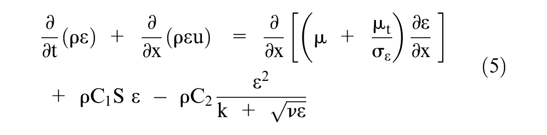
where

μ_t = turbulent dynamic viscosity,

S = modulus of the mean rate-of-strain tensor ( 27 ), and

ν = kinematic viscosity.

The model constants have accepted values of C₂ = 1.9, σ_k = 1, and σ_ε = 1.2, based on calibration to experimental data ( 26 ). Coefficient C₁ is computed as a function of k and ε according to Equation 6:

C_{1} = \max [0.43, \frac{η}{η + 5}], η = S \frac{k}{ε}

(6)

Flow Domain

The spatial relationship between a jet engine exhaust plume and a typical airfield matting system is illustrated in pseudo-three-dimensional space in Figure 6. Turbulent flow within the plume is bounded by a conical envelope that grows at a constant spreading angle θ_s. Though this system is inherently three-dimensional, for the purpose of obtaining a first estimate of matting pressure loads, the system is here approximated by a two-dimensional flow domain based on Figure 6b, neglecting flow variation along the z axis. Understanding that the error associated with this modeling choice tends to overpredict pressure loads, a two-dimensional flow domain is adopted here for its substantial advantages in computational efficiency, making possible a parametric analysis that would be impractical in three-dimensional space.

Figure 6.

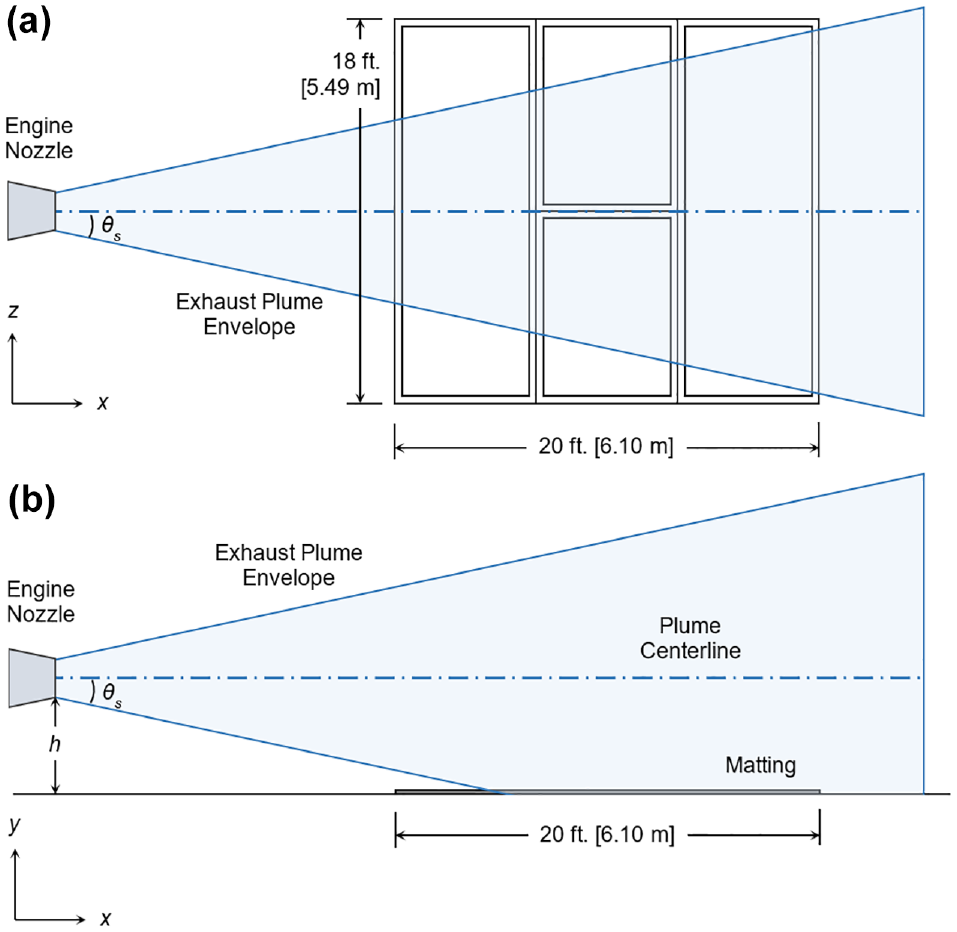
A jet exhaust plume impinging on an airfield matting system, shown in (a) plan and (b) elevation, illustrating the conical shape of the plume envelope that bounds turbulent flow. Matting measurements correspond to a medium-sized repair using fiber-reinforced polymer (FRP) panels.

The geometry of the flow domain is depicted in Figure 7, where the geometric parameters are assigned values as in Table 1. Boundary conditions are defined as follows:

Velocity Inlet : The source of the exhaust plume is the lower half of a jet engine exit nozzle of radius r, located a clear height h above pavement elevation, a distance x upstream of the leading edge of the matting system. Values assigned to r and h are comparable in scale to the engine radius and clear height of F-16 fighter jets, though it is not the intent of this study to strictly replicate any particular model of jet. Following classical subsonic jet theory, the exhaust velocity U_i is assumed to have a uniform profile, oriented normal to the boundary ( 23 , 28 ).

Pressure Inlet : The open boundary defined by the engine height h in Figure 7 is represented by a pressure inlet, located a distance x_i upstream of the velocity inlet. The value of x_i is arbitrary and serves merely to separate this boundary from the velocity inlet. Ambient atmospheric conditions are assumed here.

Pressure Outlet : The open boundary at the downstream edge of the flow domain is represented by a pressure outlet and is defined similarly to the pressure inlet. The properties of this boundary are largely arbitrary and have a negligible effect on the results if the outlet is placed a sufficient distance downstream x₀ of the matting. A suitable value of x₀ was determined by a sensitivity study.

Symmetry Boundary : The upper boundary of the domain is assigned a symmetry condition. The symmetry boundary has the effect of enforcing an idealized plume with a parallel-to-ground centerline and reduces the size of the computational domain relative to what would be needed to model the entire plume. One limitation of applying symmetry in this way is that the flow becomes artificially constrained as distance x increases, which may underestimate net pressures on the matting at larger values of x considered in this analysis.

Matting : The matting system is modeled as a rigid, impervious plate of length l and thickness t_m, with no-slip shear conditions along the boundaries. The matting thickness is set to 0.50 in. (1.27 cm), the standard thickness of both FFM and FRP matting panels ( 2 ). The length l corresponds to a medium-sized pavement repair using FRP panels.

Pavement and Cavity : The hypothesized loading mechanism of pressurization assumes the presence of a cavity below the matting. This is to be expected, since, under normal service conditions, airfield traffic subjects matting systems to repeated wheel loads in the same direction, tending to compact the back-filled repair material. Furthermore, though the matting is anchored to the existing pavement, it is not sealed in such a way as to prevent airflow through the cavity. Thus, in this model the cavity geometry is defined by four parameters: (1) cavity depth d, which is the assumed uniform depth throughout most of the cavity; (2) cavity opening depth d_e, representing the width of the openings between the matting and the pavement at the upstream and downstream ends; (3) cavity opening length l_e, which represents the length over which the matting overlaps the existing pavement at the upstream and downstream ends; and 4) cavity slope θ, an assumed constant slope at the transition regions between depth d and opening depth d_e. The pavement and cavity surfaces are solid boundaries with no-slip shear conditions.

Figure 7.

Geometric model of the flow domain and assigned boundary conditions. The matting system is modeled as a rigid, impermeable element spanning a trapezoidal cavity.

Table 1.

Geometric Parameters

Parameter	Symbol	Value
Cavity depth	d	1 in. (2.54 cm)
Cavity opening depth	d_e	Variable
Cavity opening length	l_e	Variable
Cavity slope	θ	30°
Downstream distance	x ₀	25.0 ft (7.62 m)
Engine height	h	48 in. (122 cm)
Engine radius	r	12 in. (30.5 cm)
Engine upstream distance	x	Variable
Matting length	l	20 ft (6.10 m)
Matting thickness	t_m	0.50 in. (1.27 cm)
Pressure-inlet distance	x_i	12 in. (30.5 cm)

Computational Mesh and Model Settings

The flow domain is discretized using the meshing utility in ANSYS Workbench 18.1. Across all simulations, the multizone quadrilateral-triangle method is applied with two sizing constraints specified: a maximum cell face size of 1.50 in. (3.81 cm) across the domain and a target cell face size of 0.0156 in. (0.0397 cm) along the boundaries of the matting. To refine the mesh around the matting and in the cavity, the cell growth rate is set to 1.20 along the top edge of the matting and to 1.02 along the bottom and side edges of the matting. The resulting mesh is shown in Figure 8, which depicts the local mesh resolution around the upstream edge of the matting. The total number of cells in the mesh varies as the geometry changes but is always on the order of 1 million cells. Because the output of key interest to this analysis is the distribution of net pressure along the length of the matting system, mesh adequacy is evaluated with respect to this quantity. The distributions of net pressure, represented by ΔC_p, obtained at four levels of mesh refinement are displayed in Figure 9. The mesh configuration used in this study corresponds to Curve A; the other curves are generated using increasingly coarse meshes, according to Table 2. At this level of mesh refinement, the error is judged to be negligible in light of the questions this analysis seeks to answer.

Figure 8.

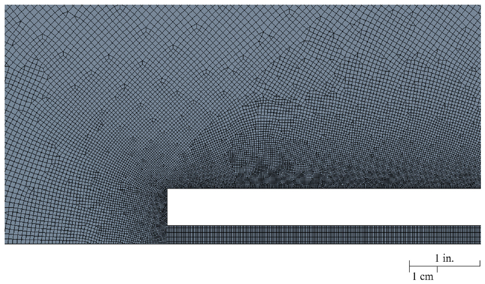
Detail view of computational mesh at the matting system upstream edge.

Figure 9.

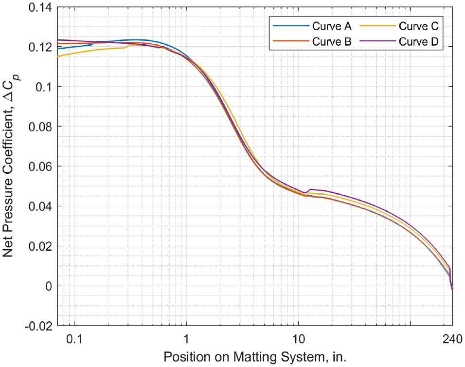
Results of the mesh convergence study presented in relation to the net pressure coefficient ΔC_p. Curve A corresponds to the mesh used in this study; the remaining curves are for meshes defined in Table 2.

Table 2.

Meshes Used in Mesh Convergence Study

Curve	Maximum cell face size, inches (cm)	Target cell face size on matting, inches (cm)
A	1.50 (3.81)	0.0156 (0.0397)
B	1.75 (4.45)	0.0208 (0.0529)
C	2.00 (5.08)	0.0313 (0.0794)
D	2.25 (5.72)	0.0625 (0.159)

The governing equations are solved in ANSYS Fluent 18.1. A steady-state solution method, which solves the time-invariant form of the RANS equations, was found to achieve adequate convergence compared with convergence obtained with a time-dependent simulation. Residuals of continuity were consistently reducible to the order of 1·10⁻³, residuals of ε were reducible to the order of 1·10⁻⁴, and the remaining residuals were generally reducible to 1·10⁻⁶ or less. The material properties of the fluid present in the flow domain are set to values typical of air—namely, density ρ is set to 0.00238 slugs/ft³ (1.23 kg/m³) and dynamic viscosity μ is set to 0.374·10⁻⁶ lb·s/ft² (0.179 mPa·s), and both quantities are assumed constant. Solutions are obtained with the pressure-based solver, using the SIMPLE pressure-velocity coupling algorithm ( 27 ). Gradients are computed using the least-squares cell-based method. Values of pressure at cell faces are calculated from cell center values using the second-order scheme to improve solution accuracy; similarly, the second-order upwind scheme is used for momentum, turbulent kinetic energy k, and turbulent dissipation rate ε.

Parameter Space

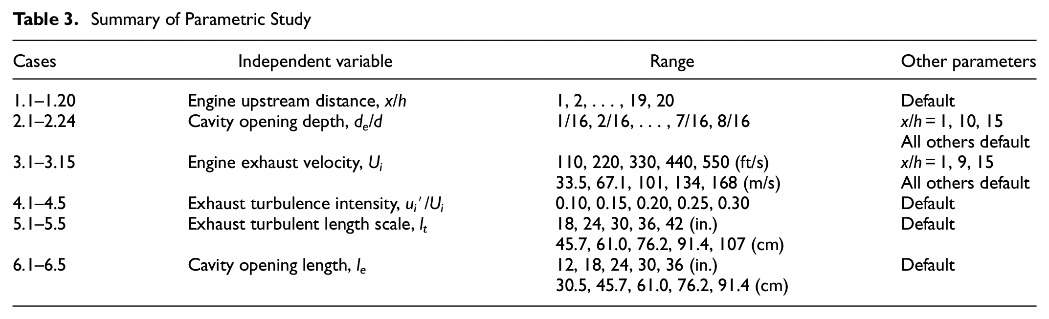
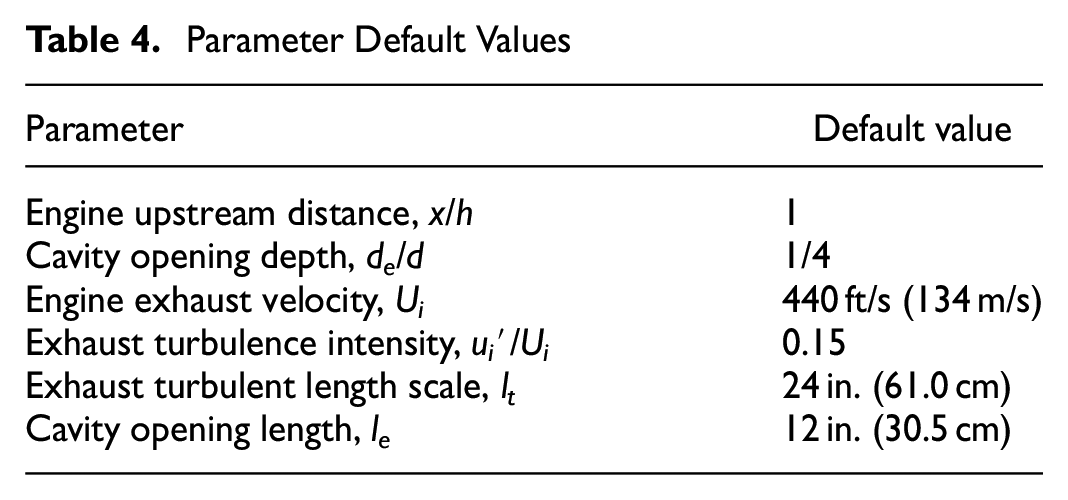
The study is organized into six case sets; in each set, one system parameter is swept over a range of values while the other parameters are held at default values. The structure of the parametric study is summarized in Table 3, which contains the contents of each case set, and in Table 4, which lists the default values assigned to the parameters. The first three case sets evaluate the sensitivity of the results to: (1) the upstream distance between the engine and the matting, represented by parameter x/h; (2) the depth of the cavity openings at the upstream and downstream edges of the matting, represented by parameter d_e/d; and (3) the engine exhaust velocity, represented by parameter U_i. Anticipating greater variability in the results because of changes in these parameters, these case sets are more exhaustive than the others. Case Sets 4–6 serve to characterize the influence of the engine exhaust turbulence intensity u_i′/U_i and turbulent length scale l_t and the cavity opening length l_e on matting pressure loads; because significantly less variability is expected to attend these parameters, only five values are considered in each of these sets. It is noted that cases are numbered in such a way that some cases are duplicates; for example, Cases 1.15, 2.20, and 3.14 are identical. Altogether, a set of 66 unique cases are evaluated in this study.

Table 3.

Summary of Parametric Study

Cases	Independent variable	Range	Other parameters
1.1–1.20	Engine upstream distance, x/h	1, 2, . . . , 19, 20	Default
2.1–2.24	Cavity opening depth, d_e/d	1/16, 2/16, . . . , 7/16, 8/16	x/h = 1, 10, 15
2.1–2.24	Cavity opening depth, d_e/d	1/16, 2/16, . . . , 7/16, 8/16	All others default
3.1–3.15	Engine exhaust velocity, U_i	110, 220, 330, 440, 550 (ft/s)	x/h = 1, 9, 15
3.1–3.15	Engine exhaust velocity, U_i	33.5, 67.1, 101, 134, 168 (m/s)	All others default
4.1–4.5	Exhaust turbulence intensity, u_i′/U_i	0.10, 0.15, 0.20, 0.25, 0.30	Default
5.1–5.5	Exhaust turbulent length scale, l_t	18, 24, 30, 36, 42 (in.)	Default
5.1–5.5	Exhaust turbulent length scale, l_t	45.7, 61.0, 76.2, 91.4, 107 (cm)	Default
6.1–6.5	Cavity opening length, l_e	12, 18, 24, 30, 36 (in.)	Default
6.1–6.5	Cavity opening length, l_e	30.5, 45.7, 61.0, 76.2, 91.4 (cm)	Default

Table 4.

Parameter Default Values

Parameter	Default value
Engine upstream distance, x/h	1
Cavity opening depth, d_e/d	1/4
Engine exhaust velocity, U_i	440 ft/s (134 m/s)
Exhaust turbulence intensity, u_i′/U_i	0.15
Exhaust turbulent length scale, l_t	24 in. (61.0 cm)
Cavity opening length, l_e	12 in. (30.5 cm)

Post-Processing

Simulation results are readily visualized by generating surface plots of flow variables as functions of location within the computational domain. A representative set of surface plots, generated using CFD-Post 18.1, are shown in Figures 10 and 11, which present part of the solution obtained for Case 1.1. The u and v components of velocity are plotted in Figure 10 to visualize the speed and direction of airflow around the upstream matting edge. An arrow plot of velocity magnitude is plotted on contours of gauge static pressure in Figure 11, illustrating the pocket of negative pressure associated with flow separation.

Figure 10.

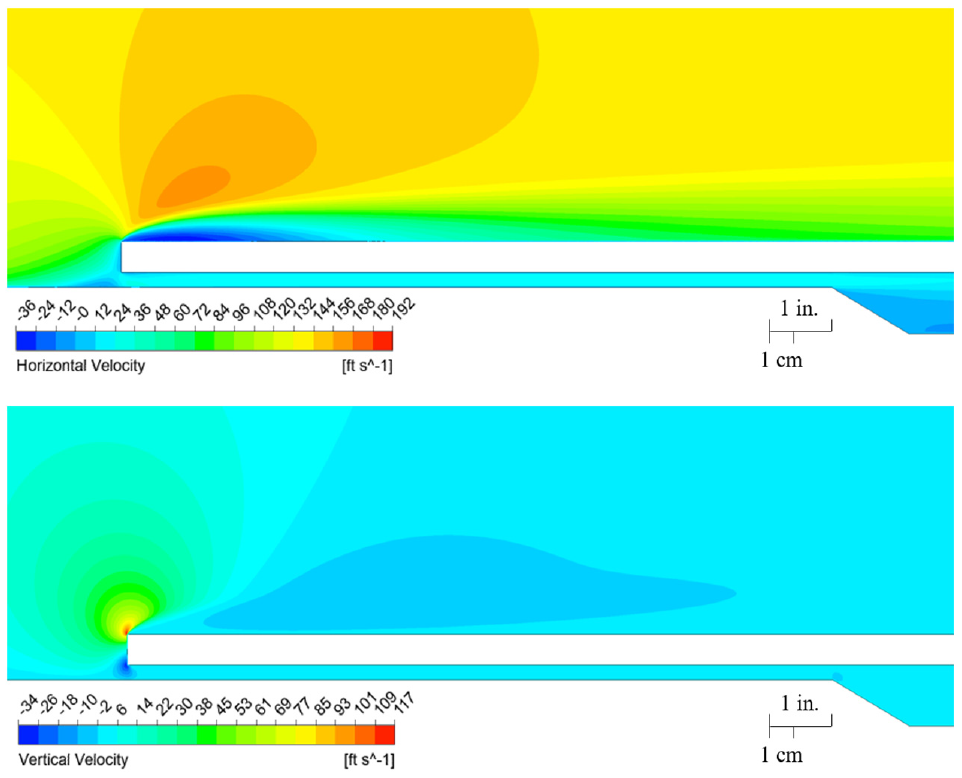
Contours of horizontal velocity u (top) and vertical velocity v (bottom) for Case 1.1, visualizing flow behavior around the leading edge of the matting.

Figure 11.

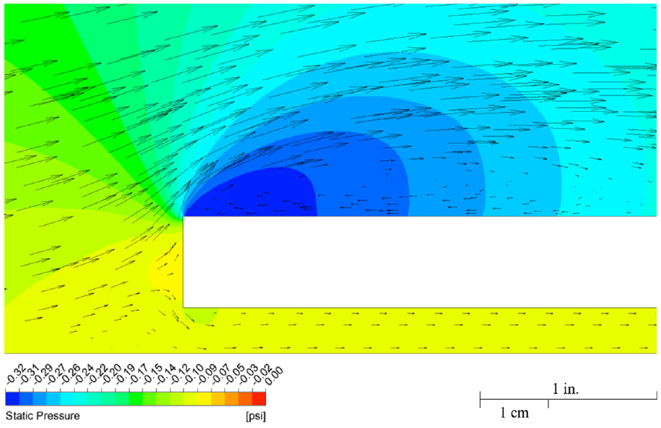
Contours of gauge static pressure underlying an arrow plot of velocity magnitude for Case 1.1. Arrow length and orientation represent the vector sum of velocity components u and v. Recirculation within the flow separation region is clearly seen.

While surface plots of pressure and velocity provide useful qualitative insights into system aerodynamic behavior, the quantity of primary interest in this study is the pressure coefficient C_p, defined according to Equation 7:

C_{p} = \frac{p - p_{r}}{\frac{1}{2} ρ_{r} v_{r}^{2}}

(7)

where

p = static pressure at a specific point,

p_r = static pressure at an arbitrary reference point,

ρ_r = reference fluid density, and

v_r = reference fluid velocity.

Since the denominator in Equation 7 is a reference dynamic pressure, C_p expresses pressure in a non-dimensional form. Furthermore, for an element subject to aerodynamic loading, the net pressure acting across the element may be quantified according to Equation 8:

Δ C_{p} = C_{p}^{'} - C_{p} = \frac{p' - p}{\frac{1}{2} ρ_{r} v_{r}^{2}}

(8)

where

$C_{p}^{'}$ and C_p = pressure coefficients computed on opposite faces of the element.

The coefficient of net pressure ΔC_p is thus the difference in static pressure normalized by a reference dynamic pressure.

The key variables for quantifying matting pressure loads are the coefficients of pressure on the top surface and bottom surface of the matting system, denoted by C_pt and C_pb, and the resulting coefficient of net pressure ΔC_p. More specifically, it is the distribution of these coefficients across the length of the matting system that is of interest. Accordingly, the static pressures computed at every discrete point along the top surface and bottom surface of the matting are exported from the simulation data file and converted to pressure coefficients C_pt and C_pb by means of Equation 7. Unless stated otherwise, in all C_p calculations, the reference density ρ_r is taken as 0.00237 slugs/ft³ (1.23 kg/m³), which is the density of air at standard temperature and pressure; the reference velocity v_r is taken as the default uniform exhaust velocity of 440 ft/s (134 m/s); and the reference pressure p_r is taken as zero. The coefficient of net pressure ΔC_p is then computed according to Equation 8 as C_pb−C_pt. For C_pt and C_pb, a positive sign indicates positive pressure—that is, +C_pt corresponds to downward pressure on the matting, and +C_pb corresponds to upward pressure. The coefficient of net pressure ΔC_p is computed such that a positive value indicates net upward pressure on the matting and a negative value indicates net downward pressure.

Results

Plotting C_pt, C_pb, and ΔC_p together as functions of position on the matting system provides a means of visualizing the influence of system parameters on pressure distributions. One such plot, presenting the pressure profiles for Case 1.1, is given in Figure 12. To remove noise caused by convergence error, these pressure profiles and all other profiles of C_pt, C_pb, and ΔC_p produced in this study have been smoothed using a rolling-average method. According to the established sign convention, the matting in Case 1.1 experiences a negative pressure on both its top and bottom surfaces, indicated by the negative C_pt and C_pb pressure curves, but the net effect is of upward pressure over most of the length of the matting, indicated by the positive ΔC_p curve. Pressure profiles have been developed for all cases listed in Table 3 and are available in the supplemental data document as Figures S1–S16. Study results are presented here in relation to force coefficients ΔC_f, C_ft, and C_fb, which represent applied force per unit width of matting and are obtained by numerical integration of ΔC_p, C_pt, and C_pb. Force coefficients are numerically equivalent to the average values of their respective pressure profiles and allow a clearer comparison of parameter influence.

Figure 12.

Pressure coefficients C_pt and C_pb and net pressure coefficient ΔC_p are plotted as functions of position for Case 1.1. Relative position along matting length is shown on the lower x axis; absolute position measured from engine nozzle is shown on the upper x axis. The sign convention dictates that positive ΔC_p corresponds to net uplift pressure.

Case Set 1: Engine Upstream Distance

A paradigm for understanding the dependence of pressure load intensity on matting position, represented by engine upstream distance x/h, is depicted in Figure 13. Based on the relative position between the matting and exhaust plume, one of three interaction states is possible:

Interaction State I. The matting is sufficiently close to the engine that no part of the matting falls within the plume envelope that bounds turbulent flow; the point of impingement is downstream of the matting. Characteristic behavior: negative gauge static pressure characterizes the top surface of the matting because of local flow separation as well as a more general suction effect arising from the proximity of the high-velocity plume; in response, negative gauge static pressure develops on the bottom surface as pressure seeks to equalize but is constrained by the size of the cavity openings, producing a net uplift pressure.

Interaction State II. The matting is positioned partially within the plume envelope; the matting is subjected to direct impingement in this state. Characteristic behavior: gauge static pressure on the matting top surface is generally negative as in Interaction State I but is driven closer to zero within the plume envelope as a consequence of direct impingement; pressure equalization again leads to negative gauge static pressure throughout the cavity; the result is that only slight, if any, net uplift pressure is possible in this state.

Interaction State III. The matting is far enough from the engine that it is completely enveloped by the exhaust plume; the point of impingement is upstream of the matting. Characteristic behavior: the matting top surface is again characterized by negative gauge static pressure in the flow separation region, but gauge static pressure approaches zero over most of the top surface; positive static pressure builds on the bottom surface as the local velocity upstream of the matting, which is greater than in States I and II, and more effectively pressurizes the cavity, resulting in net uplift over almost the entire matting length.

Force coefficients computed for Case Set 1 are plotted as functions of x/h in Figure 14. Following the interaction state paradigm, the net uplift force ΔC_f declines from x/h = 1 to x/h = 9, driven by a consistent rise in C_ft as the system moves from Interaction State I to Interaction State II, followed by a sharp increase in ΔC_f as x/h increases from 10 to 15 on transition to Interaction State III before reaching a plateau from x/h = 16 to x/h = 20.

Figure 13.

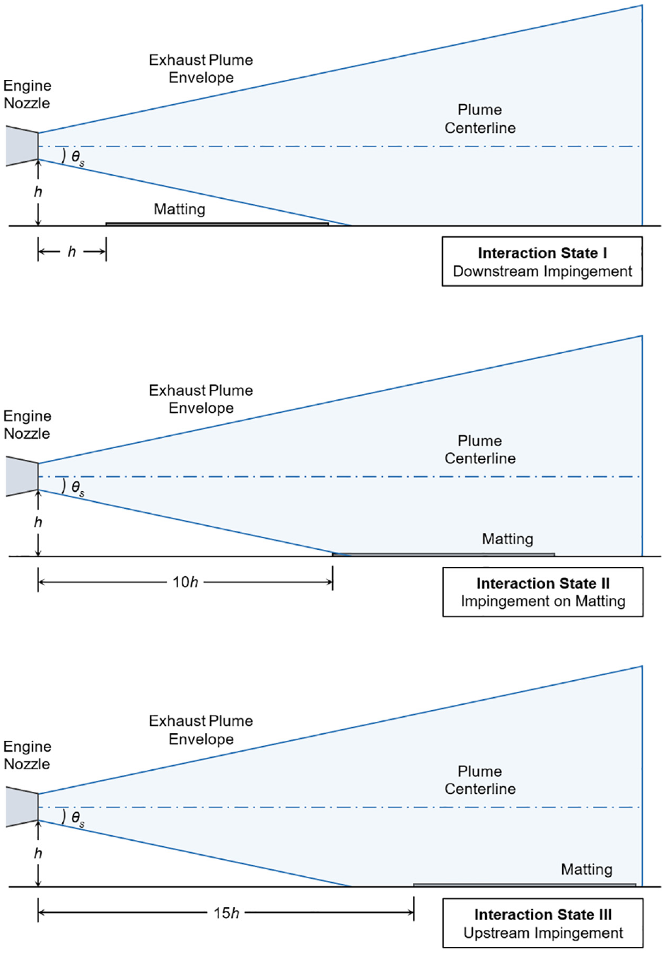
Elevation view of an airfield matting system subjected to jet exhaust plume impacts at three distances, representing three basic interaction states: impingement downstream of matting (top), direct impingement on matting (middle), and impingement upstream of matting (bottom).

Figure 14.

Force coefficients computed by integration of the ΔC_p, C_pt, and C_pb profiles for Cases 1.1–1.20, summarizing the results of Case Set 1.

Case Set 2: Cavity Opening Depth

Force coefficients computed for Case Set 2 are plotted in Figure 15. Eight cavity depth ratios d_e/d are considered at three distances x/h, corresponding to the interaction states of Figure 13. A linear fit of the net pressure coefficient ΔC_f indicates that cavity opening depth is positively correlated with net uplift pressure at each value of x/h, especially at x/h = 15 (Interaction State III). This behavior is expected, since wider openings allow for freer airflow through the cavity, with an attendant increase in cavity pressure.

Figure 15.

Force coefficients computed by integration of the ΔC_p, C_pt, and C_pb profiles for Cases 2.1–2.8 (top), Cases 2.9-2.16 (middle), and Cases 2.17-2.24 (bottom). Linear fits of the data illustrate an increase in the net uplift force ΔC_f with increasing d_e/d.

Case Set 3: Engine Exhaust Velocity

Force coefficients computed for Case Set 3 are plotted in Figure 16. As with Case Set 2, three distances x/h are considered guided by the interaction state paradigm. At x/h = 1 (State I), increasing exhaust velocity U_i magnifies the suction effect on the matting owing to proximity to the plume envelope; the increasingly negative top-surface pressure drives a rise in ΔC_f as U_i increases. At x/h = 9 (State II), which is the point of most pronounced net downward force according to the results in Figure 14, increasing velocity builds negative static pressure on the bottom surface at a greater rate than on the top surface, leading to a slight reduction in ΔC_f. Lastly at x/h = 15 (State III), ΔC_f again increases with U_i, driven by a combination of: (1) increasing negative pressure across the top surface because of more severe flow separation as velocity increases and (2) positive pressure on the bottom surface, which increases as higher-velocity airflow more effectively pressurizes the cavity.

Figure 16.

Force coefficients for Cases 3.1–3.5 (top), Cases 3.6-3.10 (middle), and Cases 3.11-3.15 (bottom).

Case Sets 4–6: Turbulence Characteristics and Cavity Opening Length

Force coefficients obtained for Case Sets 4–6 are plotted in Figure 17, illustrating the influence of exhaust turbulence intensity and turbulent length scale and the cavity opening length. In contrast to the previous three parameters, the net force ΔC_f is relatively insensitive to changes in these parameters, reflected in the near-zero slope of the linear fit of ΔC_f in all three case sets. The conclusion drawn from these data is that, within this modeling framework, the values selected for the engine exhaust turbulence characteristics and cavity opening length are of little consequence to the results.

Figure 17.

Force coefficients for Case Set 4 (top), Case Set 5 (middle), and Case Set 6 (bottom).

Estimating Anchor Forces

Because the motivating question for this study is the estimation of the worst-case anchor uplift forces that can be expected under typical service conditions, results must be expressed in relation to equivalent uplift forces. This can be accomplished by means of a tributary-area approach in which the most vulnerable anchor in the system, which would be an anchor located near the center of the upstream edge of the matting, is assumed to resist the net uplift force acting over its tributary area. This concept is illustrated in Figure 18, which depicts the specific case of a medium-sized repair using an FRP matting system but is applicable in principle to both FFM and FRP systems of other sizes. The width of the tributary area is equal to the anchor spacing of 2 ft (0.610 m) that is typical of FFM and FRP systems. Two anchors are installed near some points along the perimeter of FRP systems, including at the center of the upstream edge, but a spacing of 2 ft (0.610 m) applies for most anchors. The length of the tributary area is equal to the length of the matting system. A length of 20 ft (6.10 m), corresponding a medium-sized FRP repair, has been used as a benchmark length throughout this analysis; depending on the size of the repair site and the matting system used, the system length can range from a minimum of 13.3 ft (4.07 m) for a small-crater FRP repair to a maximum of 60 ft (18.3 m) for a large-crater FFM repair.

Figure 18.

Tributary-area approach used to estimate worst-case anchor uplift forces. The width of the tributary area is equal to the standard anchor spacing of 2 ft (0.610 m), which applies to both fiber-reinforced polymer (FRP) and folded fiberglass matting (FFM) systems.

The force acting over the tributary area is, in reality, shared by two anchors as Figure 18 indicates. Since the net pressure is never evenly distributed across the length of the system, an indeterminate analysis method would be required to determine precisely what fraction of the net force is resisted by each anchor in each case. Alternatively, for the purposes of estimating the worst-case load estimation, the load-sharing ratio may be conservatively assumed. Lastly, it is assumed that the average net force over the tributary area is equal to ΔC_f−w_d, where ΔC_f is numerically equivalent to the average value of ΔC_p in each case, and w_d is the matting dead load, approximated as 1.852 lb/ft² (88.7 Pa) based on the unit weight of FFM systems ( 2 ). Applying this procedure to the simulation results obtained for Cases 1.1–1.20, the study of engine upstream distance, x/h, yields the estimated uplift forces plotted in Figure 19, where the established sign convention in relation to uplift continues to apply. The curves in this plot are based on the results obtained for the benchmark medium-sized FRP system 20 ft (6.10 m) in length; curves representative of the other possible FRP and FFM system configurations are developed by linear scaling according to the length of each system. Since numerical solutions were obtained only for a matting length of 20 ft (6.10 m), the scaling operation gives only approximate results for the other lengths but reflects the change in net force that would be expected were these other systems to be modeled directly.

Figure 19.

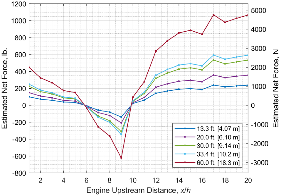
Estimated net force on the tributary area as a function of engine upstream distance x/h, computed for a tributary area of 2 ft (0.610 m) by 20 ft (6.10 m) on the assumption that the average net pressure across the tributary area is equal to ΔC_f. The computed net force accounts for an estimated dead load of 1.852 lb/ft² (88.7 Pa). System lengths correspond to five possible folded fiberglass matting (FFM) or fiber-reinforced polymer (FRP) matting configurations.

It is clear in Figure 19 that the most severe uplift demands occur at distances x/h ≥ 15, in Interaction State III. Because of the artificial variability in this range, worst-case loads are computed from Figure 19 using the mean net force in the interval x/h = 15 to x/h = 20. These net forces, since they are based on results in Case Set 1, assume a cavity opening depth d_e/d = 0.25 and an engine exhaust velocity U_i = 440 ft/s (134 m/s). Lastly, the ratio of load-sharing between the upstream and downstream anchors must be specified. It is noted that, for x/h ≥ 15, the characteristic shape of the ΔC_p profiles is weighted slightly more heavily toward the upstream edge than the downstream, because of the effect of flow separation at the upstream edge and the local negative net pressure in the downstream edge region. Thus, a load fraction of at least 0.60 for the upstream anchor seems appropriate. Worst-case anchor forces for each matting system are evaluated for load fractions from 0.60 to 1.00 in Figure 20. In summary, the methodology employed in this study finds the lower-bound worst-case anchor load to be 130 lb (581 N) in the case of a small-scale repair using FRP matting and the upper-bound anchor load to be 979 lb (4,350 N) in the case of a large-scale FFM repair.

Figure 20.

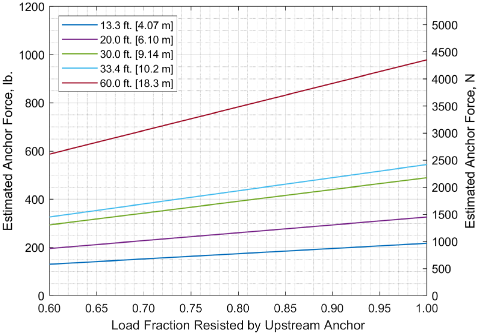
Estimated worst-case anchor uplift force as a function of load fraction resisted by the upstream anchor. The net force acting on the tributary area is drawn from Figure 19 as the mean net force in the range x/h = 15–20. System lengths correspond to five possible folded fiberglass matting (FFM) or fiber-reinforced polymer (FRP) matting configurations.

Conclusions

This study has applied a computationally efficient methodology to obtain a first estimate of exhaust-generated pressure loads on FFM and FRP airfield matting systems under typical service conditions. The key conclusions are:

Engine-to-matting distance x/h and engine exhaust velocity U_i are significant system parameters in relation to their influence on net pressure ΔC_p. Of the seven parameters considered, ΔC_p and the corresponding net force ΔC_f are largely determined by these two parameters alone. The results suggest that the most severe uplift forces occur in the state in which the exhaust plume completely envelopes the matting, for x/h ≥ 15, where ΔC_f is on average about three times the mean value of ΔC_f over the interval x/h < 15.

Cavity opening depth, represented by d_e/d, is found to be a less significant system parameter, but not negligibly so. Allowing for wider cavity openings at matting edges facilitates cavity pressurization, intensifying uplift forces. This effect is observed in the parametric study results for d_e/d at three values of x/h, where net force coefficient ΔC_f rises from 0.021 to 0.032 for x/h = 1, from 0.007 to 0.016 for x/h = 10, and from 0.036 to 0.048 for x/h = 15 as d_e/d increases from 1/16 to 1/2.

Engine exhaust turbulence characteristics u_i′/U_i and l_t and the cavity opening length l_e are found to have minimal influence on pressure loads.

Worst-case anchor uplift forces, computed according to a tributary-area approach, are estimated to have a lower bound value of 130 lb (581 N) and an upper bound value of 979 lb (4,350 N), depending on assumed load-sharing behavior among anchors and the size of the repair site.

Field testing of instrumented matting systems during jet taxi and take-off sequences is recommended as the ideal next step toward understanding system behavior and model validation.

The conclusions drawn in this work must be understood in light of the assumptions in the methodology. The nature of the assumptions is such that the error associated with them cannot be formally quantified without additional modeling using more computationally demanding approaches. Nevertheless, the assumptions can generally be grouped into two categories: those which tend to produce more conservative results, and those which, at least potentially, tend toward less conservative results. First, at least four qualities of the model may contribute to overestimation of the worst-case pressure loads, namely:

The flow domain is defined in two-dimensional space. In two-dimensional space, the system behaves as if the exhaust plume were constant in depth, rather than conical as depicted in Figure 6. It follows that the error introduced by this assumption is more significant at lower values of x/h but less significant for x/h ≥ 15, which is the range of interest for estimating worst-case forces.

The matting is modeled as a rigid element. In reality, both FFM and FRP matting systems have some degree of flexibility and deflect in response to pressure loads, and deflection tends to relieve the pressure differential. The absence of deflection thus tends to overstate ΔC_p, especially for larger matting systems.

The matting is modeled as perfectly impervious. Impermeability to airflow is a reasonable assumption for the composite panels that make up FFM and FRP matting systems, but the model does not account for the possibility of airflow through the joints between panels. Panels are bolted together during assembly but are not sealed against airflow; the presence of small openings at these joints would tend to reduce ΔC_p by facilitating pressure equalization ( 29 ).

The edges of the matting are defined by perfect right angles. The sharp corners of the matting in the geometric model are approximations and may overstate the peak in ΔC_p present at the upstream edge because of flow separation.

On the other hand, at least four aspects of the modeling approach may contribute to underestimation of pressure loads, namely:

The exhaust plume centerline is modeled by a symmetry boundary. The use of a symmetry boundary condition at the plume centerline offers computational advantages at the cost of some degree of accuracy at greater values of x/h. In reflecting the whole domain across the symmetry boundary, the solver behaves as though a mirror image of the pavement and matting were located a distance h + r above the symmetry line; thus, as distance x increases, the domain would in some respects increasingly resemble a constrained half-pipe flow. It is not expected that this behavior begins to influence the results until x is sufficiently large that the impingement of the exhaust plume with the imagined pavement surface in the upper half-plane is able to rebound to any part of the matting system in the lower half-plane. On this view, such a rebounding effect would tend to increase positive pressure on the top surface of the matting—that is, it would raise C_pt, and thereby reduce ΔC_p. Based on the conical shape of the plume envelope, it is supposed that this behavior is applicable for x/h ≥ 15, and may account for some part of the variability observed in Figures 14 and 19 for this range of x/h values.

The exhaust plume is horizontal across all cases. At most points during jet taxi, take-off, and landing sequences, incident exhaust plumes are expected to be oriented parallel to the ground or nearly so. For this reason, plume angle of attack is not taken into account in the parametric study. Nevertheless, it is recognized that during take-off the combined effects of a downward angle of attack and a plume impingement upstream of the matting may produce more severe worst-case uplift forces than those found in the present study. Future modeling efforts could account for this possible scenario.

The modeling approach does not account for transient pressure fluctuations. The steady-state solutions obtained in this study represent time-averaged pressure fields. Because the worst-case anchor forces realistically correspond to peak pressure loads produced by transient fluctuations, application of some type of peak factor to the steady-state results would be justified.

The numerical method is insufficient to represent realistic turbulent effects. The RANS analysis method adopted in this study is inadequate to represent the turbulent behavior of real jet engine exhaust plumes ( 24 ). This is closely related to the previous point, since the turbulent character of the engine exhaust is the source of the transient pressure fluctuations that would generate peak pressure loads on the matting system. The RANS method was adopted because of its computational feasibility and level of accuracy sufficient for a first estimate of exhaust-generated flow fields around matting systems. Particularly for purposes of identifying dominant system parameters and characterizing relative parameter influence on net pressure, the limitations of the RANS approach are not of great practical consequence.

Supplemental Material

sj-docx-1-trr-10.1177_03611981221145136 – Supplemental material for Modeling Exhaust-Generated Aerodynamic Pressure Loads on Airfield Matting Repair Systems

Supplemental material, sj-docx-1-trr-10.1177_03611981221145136 for Modeling Exhaust-Generated Aerodynamic Pressure Loads on Airfield Matting Repair Systems by Brandon M. Rittelmeyer, David B. Roueche, Alessandra Bianchini and James S. Davidson in Transportation Research Record

Footnotes

Author Contributions

The authors confirm contribution to the paper as follows: study conception and design: B. Rittelmeyer, D. Roueche, A. Bianchini, J. Davidson; data collection: B. Rittelmeyer; analysis and interpretation of results: B. Rittelmeyer, D. Roueche; draft manuscript preparation: B. Rittelmeyer. All authors reviewed the results and approved the final version of the manuscript.

Declaration of Conflicting Interests

The author(s) declared no potential conflicts of interest with respect to the research, authorship, and/or publication of this article.

Funding

The author(s) disclosed receipt of the following financial support for the research, authorship, and/or publication of this article: This research was supported in part by an appointment to the Student Research Participation Program at the USAF Civil Engineer Center, administered by the Oak Ridge Institute for Science and Education through an interagency agreement between the U.S. Department of Energy and AFCEC.

ORCID iDs

David B. Roueche

Alessandra Bianchini

Data Accessibility Statement

A portion of the datasets generated as part of this study is included in this published article and its supplementary file. Additional generated data are available from the corresponding author on reasonable request.

Distribution Statement

Approved for public release: distribution unlimited. AFCEC-20220028, 6 July 2022.

Supplemental Material

Supplemental material for this article is available online.

References

Rushing

J. F.

Floyd

W. C.

Rushing

T. W.

Garcia

Carruth

W. D.

Tingle

J. S.

Rutland

C. A.

Validation of FRP Matting Requirements. ERDC/GSL TR-16-22. U.S. Army Engineer Research and Development Center, Geotechnical and Structures Laboratory, Vicksburg, MS, 2016.

Airfield Damage Repair . TSPWG Manual 3-270-01.3-270-07. U.S. Air Force Civil Engineer Center, Tyndall Air Force Base, FL, 2020.

Foster

U.S., ROKAF, Combine for Airfield Damage Repair Exercise. Osan Air Base, U.S. Air Force. 2010. https://www.osan.af.mil/News/Stories/Display/Article/405557/us-rokaf-combine-for-airfield-damage-repair-exercise/. Accessed September 28, 2021.

Wade

Osan’s Airfield Damage Repair Team Exercises With Republic of Korea Air Force. Osan Air Base, U.S. Air Force. 2009. https://www.osan.af.mil/News/Stories/Display/Article/405779/osans-airfield-damage-repair-team-exercises-with-republic-of-korea-air-force/. Accessed September 25, 2021.

Jones

D. N.

Introduction to Jet-Engine Exhaust and Trailing Vortex Wakes. Technical Report 226. U.S. Air Force, Air Weather Service, 1970.

Simpson

R. L.

Turbulent Boundary-Layer Separation. Annual Review of Fluid Mechanics, Vol. 21, 1989, pp. 205–234.

Schlichting

Gersten

Boundary-Layer Theory, 9th ed. Springer, Berlin, Heidelberg, 2016.

Tafti

D. K.

Vanka

S. P.

A Numerical Study of Flow Separation and Reattachment on a Blunt Plate. Physics of Fluids A: Fluid Dynamics, Vol. 3, No. 7, 1991, pp. 1749–1759.

Essel

E. E.

Nematollahi

Thacher

E. W.

Tachie

M. F.

Effects of Upstream Roughness and Reynolds Number on Separated and Reattached Turbulent Flow. Journal of Turbulence, Vol. 16, No. 9, 2015, pp. 872–899.

10.

Bienkiewicz

Sun

Wind Loading and Resistance of Loose-Laid Roof Paver Systems. Journal of Wind Engineering and Industrial Aerodynamic, Vol. 72, 1997, pp. 401–410.

11.

J. H.

Kopp

G. A.

Modelling of Spatially and Temporally-Varying Cavity Pressures in Air-Permeable, Double-Layer Roof Systems. Building and Environment, Vol. 82, 2014, pp. 135–150.

12.

Miller

C. S.

Kopp

G. A.

Morrison

M. J.

Aerodynamics of Air-Permeable Multilayer Roof Cladding. Journal of Wind Engineering and Industrial Aerodynamics, Vol. 207, 2020, p. 104409.

13.

Cherry

N. J.

Hillier

Latour

M. E. M. P.

Unsteady Measurements in a Separated and Reattaching Flow. Journal of Fluid Mechanics, Vol. 144, 1984, pp. 13–46.

14.

Mohammed-Taifour

Weiss

Unsteadiness in a Large Turbulent Separation Bubble. Journal of Fluid Mechanics, Vol. 799, 2016, pp. 383–412.

15.

Meneveau

Mittal

Spatio-Temporal Dynamics of Turbulent Separation Bubbles. Journal of Fluid Mechanics, Vol. 883, 2020, p. A45.

16.

Johnson

F. T.

Tinoco

E. N.

N. J.

Thirty Years of Development and Application of CFD at Boeing Commercial Airplanes, Seattle. Computers and Fluids, Vol. 34, 2005, pp. 1115–1151.

17.

Fureby

Henriksson

Parmhed

Sjökvist

Tegnér

CFD Predictions of Jet Engine Exhaust Plumes. Proc. 38th Fluid Dynamics Conference and Exhibit, AIAA 2008-3727, Seattle, WA, 2008.

18.

Bui

T. T.

CFD Analysis of Nozzle Jet Plume Effects on Sonic Boom Signature. Proc. 47th AIAA Aerospace Sciences Meeting, AIAA 2009-1054, Orlando, FL, 2009.

19.

Gilmore

Jermy

CFD Study of Wake Decay and Separation Regions in Jet Engine Test Facilities. Proc. 16th Australasian Fluid Mechanics Conference, Gold Coast, Australia, 2007. pp. 436–442.

20.

Alostaz

Fantozzi

Feenstra

Innovative Jet Blast Deflector System: Analysis and Design. Proc. Structures Congress, Portland, OR, 2015. pp. 2143–2152.

21.

Munson

B. R.

Okiishi

T. H.

Huebsch

W. W.

Rothmayer

A. P.

Fundamentals of Fluid Mechanics. Wiley, Hoboken, NJ, 2012.

22.

Cao

CFD Applications in Structural Wind Engineering. In Advanced Structural Wind Engineering ( Tamura

Kareem

, eds.), Springer, Tokyo, Japan, 2013. pp. 301–324.

23.

Kaushik

Kumar

Gunasekaran

Review of Computational Fluid Dynamics Studies on Jets. American Journal of Fluid Dynamics, Vol. 5, No. 3A, 2015, pp. 1–11.

24.

Georgiadis

N. J.

DeBonis

J. R.

Navier-Stokes Analysis Methods for Turbulent Jet Flows with Application to Aircraft Exhaust Nozzles. Progress in Aerospace Sciences, Vol. 42, 2006, pp. 377–418.

25.

Wilcox

D. C.

Turbulence Modeling for CFD, 2nd ed. DCW Industries, La Cañada, CA, 1998.

26.

Shih

T.-H.

Liou

W. W.

Shabbir

Yang

Zhu

A New k-ε Eddy Viscosity Model for High Reynolds Number Turbulent Flows. Computers and Fluids, Vol. 24, No. 3, 1995, pp. 227–238.

27.

ANSYS. ANSYS Fluent Theory Guide. Ansys, Canonsburg, PA, 2009.

28.

Rajaratnam

Turbulent Jets. Elsevier Science, Amsterdam, The Netherlands, 1976.

29.

Van Schijndel

A. W. M.

Schols

S. F. C.

Modeling Pressure Equalization in Cavities. Journal of Wind Engineering and Industrial Aerodynamics, Vol. 74–76, 1998, pp. 641–649.

Supplementary Material

Please find the following supplemental material available below.

For Open Access articles published under a Creative Commons License, all supplemental material carries the same license as the article it is associated with.

For non-Open Access articles published, all supplemental material carries a non-exclusive license, and permission requests for re-use of supplemental material or any part of supplemental material shall be sent directly to the copyright owner as specified in the copyright notice associated with the article.

0.00 MB

4.11 MB