Deep Q-Network-Based Efficient Driving Strategy for Mixed Traffic Flow with Connected and Autonomous Vehicles on Urban Expressways

Abstract

With the increase in the number of automated vehicles, roads will contain a mix of automated vehicles and human-driven vehicles. At present, rule-based driving strategy control of automated vehicles in mixed traffic flow makes it difficult to obtain optimal control. Therefore, this study proposes a learning-based driving strategy for connected and autonomous vehicles under mixed traffic flow. The proposed method differs from other driving strategies in two respects. First, both the lane-change and car-following policies are included, and the Deep Q-network algorithm is utilized to train the two policies in a mixed traffic-flow environment. Second, the proposed driving strategy considers both traffic efficiency and safety when designing the reward function. Through simulation experiments, the differences in traffic efficiency and safety of this method and the rule-based method were compared and analyzed under different traffic densities and penetration rates of connected and autonomous vehicles. Simulation results show that the driving strategy improves the average velocity (by 7.02 km/h) and traffic safety (especially in high-density traffic), compared with traditional rule-based driving strategy.

Keywords

operations automated vehicles connected vehicles self-driving

With the continuous advancements in single-vehicle intelligence technology and vehicle infrastructure integration technology, connected and autonomous vehicles (CAVs) have been developed. Vehicle-to-vehicle, vehicle-to-base, and base-to-base interactions are acquired using onboard and roadside devices. This enables CAVs to obtain increasingly accurate real-time traffic data, thereby reducing traffic accidents, congestion, and trip delays ( 1 , 2 ). However, the complete replacement of human-driven vehicles (HDVs) by CAVs has not been achieved. This will lead to a mixed traffic-flow (MTF) scenario consisting of both CAVs and HDVs for a long time in the future ( 3 ). Therefore, improving transportation efficiency while ensuring traffic safety is the next major task facing MTF.

At present, there is rich experience in both domestic and international research in relation to MTF. Researchers have proposed driving strategy methods using dynamical models ( 4 ), mathematical algorithms ( 5 ), and game theory ( 6 ). With the development of onboard sensors and network connectivity technology, CAVs collect data through onboard sensors as the input to strategy methods and subsequently analyze the data to obtain a CAV-appropriate driving strategy ( 7 ). Existing non-learning-based driving strategy methods can only be used in fixed situations. On the contrary, learning-based driving strategy methods are more common; they only have to adjust the state, action, and reward functions for different scenarios for training a driving strategy to fit the target scenario. The current research on rule-based driving strategies demonstrates that rule-based approaches guarantee driving. The introduction of machine learning approaches is expected to optimize efficiency indicators while ensuring safety, further expanding the driving strategies.

Therefore, based on the existing research, this study further expands the application of Deep Q-network (DQN) in the driving strategy initialization. A CAV driving strategy was divided into lane-change and car-following policies. Based on the Markov decision process (MDP), the corresponding state parameter, action parameter, and reward function were established, in which the reward function considered traffic efficiency and safety. Subsequently, a DQN algorithm was used to solve the MDP problem. A neural network was developed for the CAV driving strategy. Finally, a simulation platform was built using MATLAB, and the reward function of the platform was verified. Under identical conditions, the DQN- and rule-based driving strategies were tested. The traffic efficiency and safety indicators (CAVs as a proportion of total traffic flow) were analyzed under different densities and CAV penetration rates, thereby validating the proposed method. The contributions of this study are as follows:

(i) A DQN-based driving strategy method developed for CAVs is applied to MTF. This method is more versatile than non-learning-based driving strategies. This implies that most common scenarios can be learned using the proposed method.

(ii) Compared with the rule-based approach, this can increase the average vehicle velocity to 7.02 km/h under all density conditions and CAV penetration situations. Particularly, in the 0 to 41 vehicle/km range and CAV penetration range of 35 to 60%, the DQN-based driving strategy increases the average velocity of MTF by 23.13 km/h, compared with the rule-based driving strategy. The proposed driving strategy improves the safety of high-density traffic based on the traffic density indicator time to collision (TTC).

(iii) The experiments in this study demonstrated that if CAVs are selected for a learning-based driving strategy in the MTF, CAVs with high penetration rates make the formulation of the driving strategy difficult. This implies that vehicles in front and back of the same lane often choose the same driving strategy. This phenomenon occurs mainly at low to medium traffic densities; that is, the vehicle itself is in an efficient driving condition. However, conflicting driving strategies between vehicles affect optimal driving behavior, leading to less efficient driving in the overall traffic flow. Thus, with low to medium traffic density conditions, moderate penetration of CAVs is more suitable than higher penetration conditions.

Review on Driving Decision-Making

Compared with HDVs, CAVs have better controllability. They can direct the entire traffic flow and improve the road efficiency by adjusting the CAV drive. The driving process of the CAVs can be divided into three steps: environmental perception, driving strategy planning, and control execution. Among these, driving strategy is particularly important in the context of MTF, that is, a complex traffic scene. At present, rule-based and learning-based approaches are often used for the driving strategy ( 7 ).

The rule-based approach combines dynamics models with experience and traffic characteristics to determine the driving strategy. Autonomous vehicles choose the appropriate driving strategy based on the scenario they are in, depending on which a multi-factor perceptional following model is proposed. This considers several factors such as vehicle synergistic optimization, velocity difference of multiple CAV vehicles, and spacing of multiple HDVs, through which the average velocity and traffic flow of the system can be effectively improved ( 4 ). Chen et al. extracted information from the strategy process of human drivers and developed a lane-changing algorithm for autonomous vehicles. It provided ideal velocity control actions and decisions in relation to whether to change lanes in real-world urban environments, while ensuring safety ( 5 ). Yu et al. proposed a lane-changing policy model suitable for autonomous vehicles in mixed environments based on the dynamic multiplayer game theory. They further proposed a hybrid splitting algorithm to obtain the Nash equilibrium solution in multiplayer games, thus obtaining the optimal strategy for autonomous vehicles’ lane-changing policy ( 6 ). Martin-Gasulla et al. investigated the phenomenon in which low penetration rates of CAVs decrease the overall vehicle throughput. They aimed to alleviate this phenomenon at urban intersections by classifying CAVs and preset green-time start-up and produced a calibrated micro simulation model using VISSIM, which can reflect this operational solution ( 8 ). Cao et al. set up a nonlinear dynamic time headway strategy for urban roads in a networked vehicle environment based on this new MTF flow. They analyzed the basic graphic model of MTF in cooperative adaptive cruise control (CACC) vehicles under different permeabilities, using CACC as a model of networked vehicles ( 9 ).

The learning-based approach involves learning from data through trial and error to obtain effective driving patterns for different road environments. Reinforcement learning is a machine learning tool that enables proxy vehicles to interact with their environment to gradually improve their driving behavior ( 10 ). You et al. modeled the interaction between autonomous vehicles and the environment as a random MDP. The driving strategies of experienced drivers were considered as the learning objectives. By designing the MDP’s reward function, the expected driving strategies of autonomous vehicles are obtained using reinforcement learning ( 11 ). However, this reinforcement learning mode can only be used in situations where the road environment is less complex, and the vehicle logic is relatively simple. Consequently, autonomous driving strategies are often combined with deep reinforcement learning to address these complex issues. As a classical deep reinforcement learning algorithm, the DQN algorithm is widely used to solve the problems associated with autonomous vehicles. Zhang et al. proposed an improved DQN lane-change policy model for autonomous vehicles. Using two neural networks with identical structure and different frequency of parameter updating to train simultaneously improved the success rate of the lane-change policy and convergence velocity of the network ( 12 ). Quek et al. used both the 2D environment built by DQN in Python and 3D environment built by Unity to control the vehicle and realized the ability of vehicle navigation and avoiding obstacles without prior information of the surrounding environment ( 13 ). Ko et al. proposed speed coordination and combined control for traffic congestion with waste of fuel consumption in bottleneck sections. They used DQN to train CAV driving behavior to alleviate traffic congestion in bottleneck sections ( 14 ).

Thus, current research on CAVs in MTF focuses on rule-based methods. Only a few studies have focused on learning-based methods. In addition, existing learning-based CAV driving strategy studies are incomplete. Only a few studies have addressed lane-changes, vehicle followings, and simultaneous impacts on traffic efficiency and safety.

Organization

This paper is organized as follows: the next section introduces the basic concept of reinforcement learning and constructs a DQN-based approach. Following this, a section establishes a simulation platform and calibrates reward function parameters, HDV driving strategy, and rule-based CAV driving strategy. There follows a section that compares and concludes a DQN-based driving strategy method with a rule-based driving strategy. The final section summarizes the study and provides its outlook.

DQN-Based Driving Strategy Methodology

The parameters for the theoretical method include input and output parameters of the CAV driving strategy, DQN algorithm, and neural network training parameters.

General Framework

The context of this research is urban expressway. CAV driving research can be approximately divided into three steps: (1) perception and data collection of the surroundings; (2) deciding whether to change lanes and plan lanes following the strategy; and (3) implementing driving behaviors.

In general, step (1) is to collect the peripheral data through onboard sensors and roadside devices.

To achieve this goal, we hypothesize that the target vehicle obtains information in relation to both the surrounding vehicles and vehicle itself in real time, ${v_{s}, v_{\max}, v_{s, f}, v_{s, b}, v_{a, f}, v_{a, b}, d_{s, f}, d_{s, b}, d_{a, f}, d_{a, b}}$ .

Step (2) comprises the main content of this research. In this paper, the two steps for CAVs in lane-change policy and CAV following policy are simplified. The lane-changing policy is first considered, followed by the car-following policy attributable to the difference of the former decision, resulting in different environment status data. However, the lane-change policy as the first step is used to predict the nature of the assumptions. It does not necessarily imply that the CAV will undergo lane changing. In the actual driving process, CAV lane-change behavior and following behavior are considered simultaneously.

In the initial phase, the CAV does not have any effective lane-change or car-following driving behavior. Rather, it has a driving behavior that benefits the most from trial and error under different environmental conditions. The lane-change and vehicle-following policies are based on the DQN algorithm. The entire algorithm is divided into two stages. The first stage is Q-learning training, in which the CAV selects reward functions from different actions in different environments, which are stored in tabular form. The second stage is neural network training. The corresponding neural network is learned and generated using the value function matrix of the action state obtained in the first stage.

In this study, the driving strategy in step (2) is implemented in a considerably short time. Thus, no specific research on step (3) was presented. Instead, the CAV is set to drive directly to the appropriate spot in the moments following lane-change or car-following policies. This ignores the details of vehicle movements between these two moments. The overall framework is shown in Figure 1.

Figure 1.

General framework.

Reinforcement Learning

The basic framework for reinforcement learning is the MDP ( 15 ). The simplest MDP comprises four tuples: state S, action A, reward function R, and transition probability P. The MDP provides an agent with an arbitrary state $s \in S$ in which the agent chooses an action with a certain transfer probability P. After completing the action $a \in A$ , the agent reaches a new environmental state and gives a reward value R.

DQN-Based Lane-Change Policy Parameter

Here, the state parameters for the CAV lane-change policy include: the distance between the target vehicle and front of the current lane $d_{s, f}$ ; distance between the target vehicle and front of the adjacent lane $d_{a, f}$ ; velocity of vehicle in front of the target vehicle in the current lane $v_{s, f}$ ; velocity of the car in front of the target vehicle in the adjacent lane $v_{a, f}$ ; and whether the lane adjacent to the target vehicle is empty, $f_{empty}$ .

s_{lc} = {d_{s, f}, d_{a, f}, v_{s, f}, v_{a, f}, f_{empty}}

(1)

Because this study deals with the dual carriageway of an urban expressway, the target vehicle only needs to consider whether it needs to change lanes.

a_{lc} = {lane change, no lane change}

(2)

To ensure that the CAV can change lanes under the premise of sufficient lane-change space, we consider the following two aspects before the lane-change behavior to account for the reward function of the lane-change policy.

Equation 3 considers whether there are other vehicles in an identical position on the adjacent carriageway of the current target vehicle. Suppose that there are two vehicles driving in parallel in the adjacent lanes, and a better driving space exists for one car in front of the other. According to driving habits, for driving safety reasons, the first car will not forcefully overtake to change lanes. Therefore, the reward function is set as follows: if there are no other vehicles, a reward $R_{1}$ will be granted; otherwise, the lane change of the target vehicle will cause considerable interference such that a larger penalty $P_{1}$ will be imposed.

r_{empty} = {\begin{matrix} R_{1}, f_{empty} = 1 \\ P_{1}, f_{empty} \neq 1 \end{matrix}

(3)

Equation 4 considers whether the lane change of the target vehicle is influenced by the distance to the future driving space ( 16 ). CAVs have more road traffic data than HDVs do. Thus, they can consider how fast a vehicle is moving in the front or adjacent lane of the current lane during the decision stage. They can judge whether to change lanes based on the velocity of the current and next lane and the longitudinal distance between the target vehicle and the vehicle in front of it. This implies that if the target vehicle chooses a lane that provides more driving space in the future, there is a larger incentive. This reward function is defined using the longitudinal distance between the vehicle in front of the selected lane and the target vehicle as well as the distance traveled by the vehicle in a future time step.

r_{space} = {\begin{matrix} d_{s, f} + v_{s, f} T, lane no change \\ d_{a, f} + v_{a, f} T, lane change \end{matrix}

(4)

The reward function of the lane-change decision consists of two small reward functions.

r_{lc} = r_{empty} + r_{space}

(5)

DQN-Based Car-Following Policy Parameter

The CAV following policy presented here is formulated by the state parameters, including the target vehicle current velocity $v_{s}$ , target vehicle maximum velocity, velocity of the target vehicle at the next moment $v_{target}$ , distance between the target vehicle and front of the current lane $d_{s, f}$ , distance between the target vehicle and back of the current lane $d_{s, b}$ , velocity of the vehicle in front of the target vehicle in the current lane $v_{s, f}$ , and velocity of the car behind the target vehicle in the current lane $v_{s, b}$ .

s_{following} = {v_{s}, v_{\max}, v_{target}, d_{s, f}, d_{s, b}, v_{s, f}, v_{s, b}}

(6)

To optimize the calculation process, the original acceleration-oriented calculation was changed to a velocity-oriented calculation. It provides the CAV with six velocity options to increase its dynamic changes. Subsequently, the velocity interval ranged from the minimum to the maximum velocity. The minimum velocity is zero, and the maximum velocity is set according to road requirements.

a_{following} = {v_{0}, v_{1}, v_{2}, v_{3}, v_{4}, v_{5}}

(7)

To ensure that a CAV can maximize the driving efficiency under the premise of safety, the reward function of the car-following policy in this paper includes four aspects, including traffic safety of the CAV, driver’s comfort, driving distance and velocity limits.

Equation 8 considers the traffic safety of the CAV on the road, similar to the cellular automata model ( 17 ) presented by Taniguchi and Suzuki, which includes the TTC; a lower TTC value corresponds to a higher probability of danger. Therefore, the value must be inverted to ensure positive correlation with the reward function. To ensure the maximum security of the CAV, if the determined velocity of the CAV at the next moment is reduced, and the vehicle spacing in the front gives a reward $R_{2}$ , assuming that the target vehicle in front of the vehicle stops in the next moment, the TTC is calculated. The result is multiplied by the reciprocal of the TTC value and penalty value $P_{2}$ .

TTC = {\begin{matrix} \frac{d_{s, f} - d_{l}}{v_{s} - v_{s, f}}, v_{s} > v_{s, f} \\ + \infty, v_{s} \leq v_{s, f} \end{matrix}

(8)

r_{ttc} = {\begin{matrix} R_{2}, v_{target} < d_{s, f} \\ \frac{v_{target}}{d_{s, f} - d_{l}} P_{2}, v_{target} \geq d_{s, f} \end{matrix}

(9)

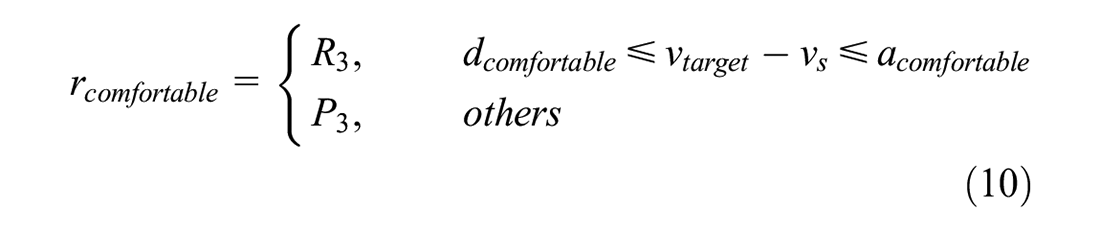
Equation 10 considers the impact of velocity changes on the driver’s comfort. The magnitude of the acceleration is closely related to the decision-making and control of autonomous vehicle systems. Jin et al. analyzed the interaction between passengers and autonomous vehicle systems ( 18 ). They proposed an acceleration control strategy for autonomous vehicles and divided the driving comfort into different acceleration intervals, stipulating that accelerations above 2 m/s² are significantly uncomfortable. If the acceleration of the target vehicle is in the comfort zone, a reward $R_{3}$ is assigned. Otherwise, a small penalty $P_{3}$ is imposed.

r_{comfortable} = {\begin{matrix} R_{3}, d_{comfortable} \leq v_{target} - v_{s} \leq a_{comfortable} \\ P_{3}, others \end{matrix}

(10)

Equation 11 represents how the velocity and distance are used as a value function ( 19 ) when studying the car-following policy based on reinforcement learning to ensure that the CAV can travel at a certain velocity on the road. Therefore, the distance that the CAV can drive in the next time step is also a reward function for the following decisions in the text.

r_{distance} = v_{target} T

(11)

As different vehicles have different driving functions, they require velocity limits. Equation 12 ensures that the target vehicle does not choose to move faster than its maximum velocity limit. Within this limit, a reward $R_{4}$ is provided. Otherwise, a larger penalty $P_{4}$ is imposed.

r_{constra int} = {\begin{matrix} R_{4}, v_{target} < v_{\max} \\ P_{4}, v_{target} \geq v_{\max} \end{matrix}

(12)

The reward function for subsequent decisions consists of the four small reward functions.

r_{following} = r_{ttc} + r_{comfortable} + r_{distance} + r_{constra int}

(13)

DQN Algorithm

After setting up the three elements of the MDP, the function of the state action value is calculated using the Q-learning algorithm and stored in a Q-table. However, this method is feasible in environments with only few actions and states. Modeling CAV scenarios requires a relatively complex environment. Thus, the Q-table becomes significantly large. Additionally, it is inconvenient to call data if the values of the corresponding operations are stored in all different states in the Q-table. Therefore, we chose the neural network DQN algorithm based on the Q-learning algorithm. Based on the input stochastic state condition, the neural network is used to approach the state action value function and output the corresponding state action value under different actions. Finally, the CAV selects the action corresponding to the maximum value.

DQN Algorithm
Input: S, a, R, α, γ
Output: Q-network
01: $Q \leftarrow Q_{0}$
02: Repeat (for each episode):
03: Random generation $s$
04: Repeat (for each a from A):
05: Take action $a$ , Observe $r, s'$
06: $R (s, a) \leftarrow r, s \leftarrow s'$
07: Repeat (for each $a'$ from A):
08: Take action $a'$ , Observe $r$
09: $Q (s', a') \leftarrow r$
10: Until $a'$ is terminal
11: $Q (s, a) \leftarrow Q (s, a) + α [R (s, a) + γ \max Q (s', a') - Q (s, a)]$
12: Perform a gradient descent step
$L (θ) = {(r + γ_{a'}^{\max} Q^{} (s', a', θ^{}) - Q (s, a, θ))}^{2}$
13: Update $θ$ , Q-network
14: Until s is terminal
15: Until episode is terminal

DQN Training

Here, machine learning and deep learning applications in MATLAB were utilized to train the DQN-based lane-change and car-following policies. There were five and seven inputs and two and six outputs for the two neural networks, respectively. The number of neurons in the hidden layer was set to ten based on the empirical formula for determining the number of neurons in the hidden layer. The number of nodes in the hidden, input, and output layers are represented by h, m, and n, respectively. $α$ is the ideal 2–10 adjustment constant.

h = \sqrt{m + n} + α

(14)

The complexity of subjects determines the number of hidden layers. The neural network was trained by setting different layers of hidden layers, comparing the training results and training time, and finally setting the hidden layers to two. Trainlm is the default algorithm in MATLAB, which has the fastest convergence speed among medium-sized neural networks. Other neural network parameters are the default parameters of the system as shown in Table 1.

Table 1.

Parameter Specification

Parameter symbols	Parameter descriptions

CAV driving strategy input variables
$v_{s}$	Target vehicle current velocity
$v_{\max}$	Target vehicle max velocity
$d_{s, f}$	Distance between the front-end of the target vehicle and front-end of the adjacent vehicle in the current lane
$d_{s, b}$	Distance between the front-end of the target vehicle and front-end of the adjacent-rear vehicle in the current lane
$d_{a, f}$	Distance between the front-end of the target vehicle and front-end of the adjacent vehicle in the adjacent lane
$d_{a, b}$	Distance between the front-end of the target vehicle and front-end of the adjacent-rear vehicle in the adjacent lane
$v_{s, f}$	Velocity of vehicle in front of the target vehicle in the current lane
$v_{s, b}$	Velocity of the car at the back of the target vehicle in the current lane
$v_{a, f}$	Velocity of the car in front of the target vehicle in the adjacent lane
$v_{a, b}$	Velocity of the car at the back of the target vehicle in the adjacent lane
$f_{empty}$	Whether lane adjacent to the target vehicle is empty
$d_{l}$	Standard vehicle length
T	Time step
CAV driving strategy output variables
$v_{target}$	The velocity of the target vehicle at the next moment
Lane-change	Takes 1 for change; Takes 0 for no change.
DQN algorithm parameters
$s_{i}$	ith state
$a_{i}$	ith action
$r_{i}$	ith reward function
$R_{i}$	ith reward value
$P_{i}$	ith penalty value
$Q (s, a)$	State-value function
$L (θ)$	Loss function
$θ, θ^{*}$	Weights for neural networks
$γ$	Discount factor
Neural network parameter
Number of hidden layers and neurons	[10,10]
Maximum number of epochs to train	1,000
Performance goal	0
Maximum validation failures	6
Minimum performance gradient	1e-7
Initial learning rate	0.001
Learning rate decrease factor	0.1
Learning rate increase factor	10

Note: CAV = connected autonomous vehicle; DQN = deep Q-network.

Figure 2 shows how the loss function varies with the number of iterations during neural network training for both policies (set to 1,000). The loss function was no longer reduced (reaching the best value), and the training was completed. The average loss function of the training (blue line), validation (green line), and test (red line) sets were no longer reduced at the 1,000th lane-change policy iteration or approximately the 750th car-following policy iteration.

Figure 2.

Number of training iterations: (a) Training iterations for lane change policy and (b) training iterations for car following policy.

Experimental Platform Construction and Other Vehicle Parameter Settings

Experimental Environment Setting

Considering the abundance of two-lane city roads and given that a two-lane city road can meet the minimum requirements for changing lanes and accompanying vehicles, this study considers a two-lane city expressway to be the research background.

In this study, a simulation platform to verify the validity of this method was established using the cellular automaton model ( 20 ). Because traffic participants are discrete in nature, using cellular automaton theory to simulate lane-change and car-following policies effectively avoids the approximation transition between discrete–continuous–discrete. The theory was proved to be feasible ( 21 ). To better simulate traffic flow on one-way two-lane city freeways, we referred to the simulation criteria of the cellular automaton model developed by Rickert et al. ( 22 ). Each cell was 7.5 m long and 3.5 m wide. Each road was circular and comprised 1,000 cells, with a total length of 7.5 km and simulation time of 1,000 s. To ensure the safety of vehicle and influence of its factors, the length and width of the CAV and HDV were set to 5 and 1.8 m, respectively. Assuming the vehicle was always at the center of the cell space, that is, the vehicle was 1.25 m from both the upper and lower edges of the cell space, there was a safe distance of 2.5 m between the vehicle and cell, which was maintained even if the vehicle was in two adjacent cells at the front and back. The cell space size as well as the vehicle length were maintained at such a size that the cell length was neither too short to accommodate a vehicle nor too long to cause the vehicle movement to change too fast, and the overall traffic flow change could be reflected roughly under that condition.

In the initial stage of the simulation, vehicles are generated at random locations in the cell space according to a certain CAV permeability and traffic density. Each vehicle was given an initial maximum velocity in the range of three to five cell length/s, that is, 81, 108, and 135 km/h, to ensure that the vehicles running on the simulated road meet the different maximum driving velocity of real vehicles resulting from their driver characteristics and vehicle characteristics. Each vehicle obtained its real-time velocity by multiplying its maximum velocity with a random value between 0 and 1 and rounding up.

Owing to the nature of the cellular automaton model, the vehicle directly performs the following lane-change behaviors to achieve cell-to-cell state transfer, that is, the vehicle does not stop in the middle of two longitudinal cells or between two transverse cells at the next moment. Instead, it directly reached the next cell, and only one vehicle could exist in each cell at a moment during the simulation. The velocity intervals of all types of vehicles were zero to five cell length/s, that is, 0, 27, 54, 81, 108, and 135 km/h. The road and vehicle settings are shown in Figure 3.

Figure 3.

Simulation platform construction.

Reward Function Parameter Calibration

In the previous section, the settings of the reward function related to the DQN lane-change and car-following policies were developed. However, the reward and penalty values had to be further calibrated. In this study, we first assigned values to the reward and penalty using the enumeration method, that is, $R_{i} \in (1, 5), P_{i} \in (- 10, - 1)$ . The reward and penalty values are any integer located in the domain value interval. The decision scheme of the values is then trained, and the neural network obtained from the training results is used in the simulation platform. The simulation will be used to obtain the total average vehicle velocity $V_{total, mean}$ , number of remaining vehicles $N_{vehicle, surplus}$ , and acceleration variation $Δ a_{total, mean}$ . These are the calibrations of the reward function parameters used to measure results. The larger the total average vehicle velocity, the better the calibration of this parameter. The more remaining vehicles, the less cars will collide with each other, calibrating this parameter. The more frequent the acceleration variation, the worse the parameter calibration results are for driver experience.

In this study, the process was repeated 10,000 times to arrive at a matrix that links rewards and penalties to the overall average vehicle velocity, number of remaining vehicles, and acceleration variation.

[R_{1}, R_{2}, R_{3}, R_{4}, P_{1}, P_{2}, P_{3}, P_{4}, V_{total, mean}, N_{vehilce, surplus}, Δ a_{total, mean}]

(15)

After completing the data statistics, the three indicators were normalized. Consequently, the indicators were of the same order and easy to compare and analyze.

X^{'} = \frac{X - \min (X)}{\max (X) - \min (X)}

(16)

Finally, three metrics were summarized. The reward and penalty values corresponding to the maximum value were selected as the correction results of the reward function parameters. $R_{1}$ , $R_{2}$ , $R_{3}$ , $R_{4}$ , $P_{1}$ , $P_{2}$ , $P_{3}$ , and $P_{4}$ are 1, 1, 5, $1$ , −8, −5, −2, and −9, respectively.

Other Vehicle Parameters

In MTF, there are HDVs in addition to CAVs. Thus, it is necessary to set up lane-change and car-following models for HDVs. Simultaneously, to verify the validity of the DQN-based driving strategy, it must be compared with the traditional CAV lane-change and car-following policies.

In relation to the HDV lane-change decisions, the single-lane random cell automaton (STCA) traffic model proposed by Chowdhury et al. ( 23 ) was adopted in this study. The model stipulates that if the target vehicle

(i) does not have sufficient driving space in front of its current lane for it to continue at its current velocity at the next moment;

(ii) the adjacent lane has better driving space than that lane; and

(iii) there is no interference from other vehicles (as the change of vehicle state in the cellular automaton model is done instantaneously from the current moment to the next moment, the rule ensures that there is space to perform a lane change in the adjacent lane where the vehicle is located, which in turn ensures the safety of the vehicle),

then the target vehicle changes its lane, and the lane-change then updates the rules as per Equation 17.

f_{lc} = {\begin{matrix} \begin{matrix} lane change, v_{s} + 1 > d_{s, f} and \\ d_{s, f} < d_{a, f} and \\ f_{empty} = 1 \end{matrix} \\ no lane change, others \end{matrix}

(17)

For the HDV car-following policy, we chose the rule-based STCA proposed by Nagel and Schreckenberg ( 20 ). In this model, each cell can be either occupied by a car or be empty. Each car was assigned a velocity between 0 and $v_{\max}$ but must not exceed $v_{\max}$ . The status of each cell is updated at each time step. The model stipulates that if the target vehicle is in the current lane, conditions exist ahead for the vehicle to accelerate, and the velocity of the vehicle after acceleration does not exceed its maximum limit, the target vehicle accelerates. That is, the current vehicle driving velocity does not exceed the maximum limit, and the driving space in front of the vehicle meets the driving distance after acceleration, and the vehicle accelerates. Similarly, if the forward travel space of the target vehicle is not conducive to maintaining the current velocity, the target vehicle should decelerate. That is, the front driving space is no longer able to meet the current vehicle at the current velocity, and the vehicle slows down.

As a result of the constraints, the HDV is affected by the distance of the vehicle in front of it, thus always maintaining a safe distance greater than or equal to the length of one cell from the vehicle in front of it during driving. The vehicle update rules are as follows:

v_{target} = {\begin{matrix} v_{s} + 1, v_{s} < v_{max} and v_{s} + 1 < d_{s, f} \\ d_{s, f} - 1, v_{s} > d_{s, f} \end{matrix}

(18)

According to the manual vehicle driving test conducted by Sugiyama et al. ( 24 ), at the start of the race, manual vehicles are evenly distributed on the loop and travel at a uniform velocity. However, owing to uncertainties, some vehicles always slow down. This makes it impossible for the entire platoon to maintain uniform velocity. According to this characteristic, combined with the random deceleration rules in the STCA model, an artificially driven vehicle, whose velocity is not zero after implementing the lane-change and car-following policies, is decelerated with probability $P_{r}$ . Each deceleration size is one cell length per second, where $P_{r}$ is 0.1.

v_{target} = {\begin{matrix} v_{target} - 1, v_{target} > 0 and rand < P_{r} \\ v_{target}, other \end{matrix}

(19)

Considering the CAV lane-change policy, the rule-based lane-changing model ( 16 ) proposed by Jin et al., which refers to the reward function of the lane-change policy based on DQN, was adopted here. Depending on the mode of lane-change, the size of the vehicle’s future driving space determines whether a lane-change is required at this moment. The vehicle will move to the lane that provides more space at the next moment when the target vehicle is in the current lane. $D_{S}$ indicates the distance the target vehicle travels in the current lane at the next moment, and $D_{a}$ indicates that in the adjacent lane in the next moment.

D_{s} = d_{s, f} + (v_{s, f} + a_{s, f}) T

(20)

D_{a} = d_{a, f} + (v_{a, f} + a_{a, f}) T

(21)

f_{lc} = {\begin{matrix} lane change, D_{s} < D_{a} and f_{empty} = 1 \\ no lane change, others \end{matrix}

(22)

In relation to the CAV following decision, we adopted the intelligent driver model (IDM) proposed by Treiber et al. ( 25 ). The model consists of two parts: the acceleration trend in automatic state and the deceleration trend considering head-on collision. $v_{d}$ , $d_{safe}$ , $a_{\max}$ , and $b_{\max}$ are the expected velocity, safe distance, maximum acceleration, and maximum deceleration, respectively.

v_{target} = v_{s} + a_{s}

(23)

a_{s} = a_{\max} (1 - {(\frac{v_{s}}{v_{d}})}^{δ} - {(\frac{d^{*} (v_{s}, v_{s, f})}{d_{s, f}})}^{2})

(24)

d^{*} (v_{s}, v_{s, f}) = d_{safe} + v_{s} T + \frac{v_{s} (v_{s} - v_{s, f})}{2 \sqrt{a_{\max} b_{\max}}}

(25)

In this study, the acceleration for each step length is calculated using the IDM. As the IDM was originally used for continuous traffic flow, and the platform simulated in this study was discrete, the simulation time was divided into several small time steps. The acceleration of the vehicle under each small step is calculated using the IDM, such that the sum of the velocity and acceleration of the vehicle cannot exceed the maximum acceleration. The final acceleration is the max integer upward to fit the measurement of the cellular automata model.

Results and Discussion

To verify the effectiveness of the DQN-based driving strategy, the aforementioned rule-based lane-change model and IDM car-following model was combined to obtain the rule-based driving strategy. Both strategies were tested on a simulation platform with different initial traffic densities (two-lane urban expressway conditions at 0–226 vehicles/km) and CAV penetration rates (0%–100% CAV penetration rate). Each experiment was repeated 100 times. Each simulation time was set to 1,000 s under different initial conditions. At each time step, based on different driving strategies, traffic data were used to perform the corresponding driving behavior. The velocity and calculated TTC value were recorded the next moment after the execution.

Traffic Efficiency

The average velocities of the CAVs, HDVs, and other vehicles were chosen as the performance indicators for traffic efficiency. As shown in Figure 4, the horizontal and vertical coordinates on each small graph indicate the two-lane traffic density and CAV penetration rate, respectively. The average velocity of the corresponding vehicle was calculated for each traffic density and CAV penetration and visualized using different colors. The blue and red lines indicate faster and lower average velocities, respectively. The graph directly reflects the change in the running state of the entire traffic flow.

Figure 4.

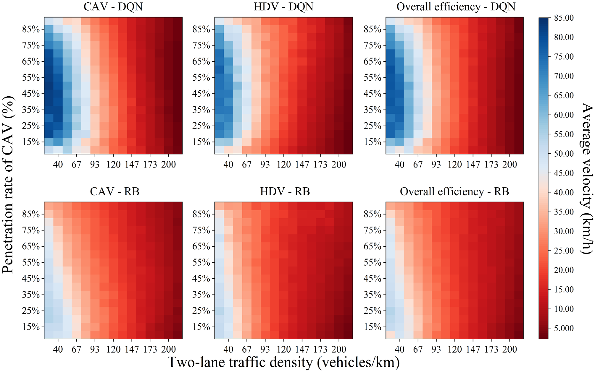
Travel efficiency analysis.

Horizontal coordinate analysis demonstrated that when the traffic density was between 0 and 82 vehicles/km, the DQN-based CAV driving strategy had significant advantages over the rule-based driving strategy in all three indices. This is because the DQN-based driving strategy completed all of its driving actions during the training phase of a potential driving environment to achieve the optimal driving behavior in that environment. An approach was designed to optimize the outcomes of different driving behaviors. The rule-based driving strategy had only one driving behavior in the form of a calculation of the acquired data in the actual driving situation. The method was oriented only to the optimal solution of the calculation formula. DQN-based CAVs can better adapt to the traffic-flow environment under medium and low traffic densities by increasing their own velocity to increase the overall average velocity. This ultimately improves the overall average velocity of all vehicles. Simultaneously, changes in the velocity of CAVs affect the overall traffic flow, changing the velocity available for HDVs.

Considering the vertical coordinate change analysis under the CAV driving strategy proposed here, a larger CAV penetration rate is not preferable. However, a rate within the interval of approximately 35 to 60% is advantageous. The explanation for this is that a DQN-based CAV will choose the best driving behavior in a situation where the traffic density is low, that is, the vehicle has the opportunity to choose its velocity. If there is a CAV in front of the vehicle, the two will often make identical driving decisions in the environment they are in. If the maximum speed of the front CAV is lower than that of the rear CAV, the velocity of the rear CAV is prevented from increasing, causing a chain reaction that reduces the average velocity across the road.

Taking the average overall vehicle velocity in the interval of 0 to 82 vehicles/km and a CAV penetration rate between 35% and 60%, the average overall vehicle velocity of the DQN-based driving strategy reaches 60.81 km/h. In contrast, that of the rule-based driving strategy only reaches 37.68 km/h, that is, a difference of 23.13 km/h. Therefore, the DQN-based driving strategy is more traffic-efficient compared with the rule-based driving strategy.

Presently, CAVs are being developed to bring a more efficient way of travel. However, current CAVs rely only on the information obtained by their sensor equipment to make driving strategies conducive to driving. They do not have a system–body unified scheduling for all CAVs. In this context, the above experimental results are not significantly advantageous for developing single-vehicle intelligence in the mainstream direction promoted today. As CAVs account for an increasing share of road traffic, CAVs will likely adopt conservative measures to drive at low velocities on roads with high CAV penetration. Therefore, a single-vehicle intelligence approach, similar to the one in this study, does not apply to high penetration. Future research on CAV technology should not be limited to single-vehicle intelligence. Rather, it should be directed toward multi-vehicle collaboration to avoid conservative driving behavior ( 26 ). CAV manufacturers can start from the cooperative driving of two vehicles and expand to multiple vehicles. This method can finally expand to the entire road or even the entire road network of all CAV cooperative driving to make the whole area of travel efficient.

To ensure the reliability of the above experimental results, we used the VISSIM microscopic simulation platform for secondary development to evaluate the simulation results of DQN-based driving decisions in the cellular automaton model. Combined with the experimental design of the cellular automata model and considering the limitations of the VISSIM simulation platform itself, the following adjustments were required:

Owing to the limitations of the VISSIM simulation platform, the vehicle input changed from two-lane traffic density to two-lane traffic flow.

To accommodate the different maximum driving velocities of vehicles assumed in the cellular automata model, the expected velocities of the initial input vehicles were distributed equally according to the classification of 60, 70, 80, 90, and 100 km/h.

With the exception of vehicles based on the DQN driving strategy, all vehicles complied with the VISSIM driving rules.

The final simulation results of the VISSIM platform are similar to those of the cellular automata model platform. The average velocities of vehicles with a medium CAV penetration rate were optimal under low- and medium-flow conditions, as shown in Figure 5.

Figure 5.

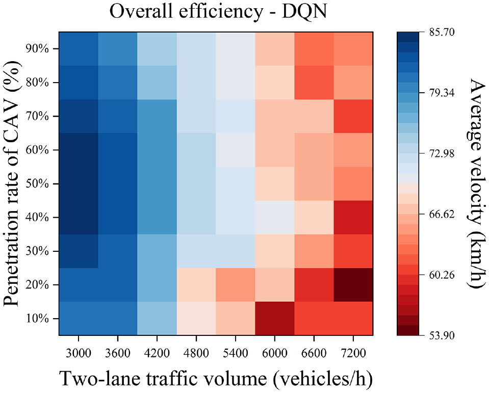
VISSIM simulation platform evaluation experimental results.

Traffic Safety

Assessment of vehicle traffic safety includes the presence of single-behavior threat metrics, optimization methods, formal methods, probabilistic frameworks, and data-driven approaches, such as machine learning ( 27 ). Considering the application scenario of this paper, the TTC index is chosen as the traffic safety assessment criterion ( 28 ). When considering traffic safety, vehicles with a TTC index of less than 1.5 s are identified as having a higher rear-end collision risk factor. Furthermore, the ratio of the number of vehicles to the total number of vehicles is an assessment.

R_{TTC} = \frac{N_{risk}}{N_{total}}

(26)

Under different traffic density conditions and CAV penetration rates, DQN-based driving strategy and rule-based driving strategy methods were adopted, respectively. No collisions occurred during the experiment. The experimental results show that the ratio of rule-based driving strategy to high-risk vehicles was approximately zero under low traffic density conditions. That of the DQN-based driving strategy method can be maintained at low values. Under moderate traffic density conditions, the proportion of high-risk vehicles increases with an increase in penetration rates in both vehicles. The performance of the DQN-based driving strategy method was more stable at high densities, with the CAVs remaining at low operational levels. The proportion of high-risk vehicles was within a reasonable range for CAV penetration. Contrastingly, the performance of the rule-based driving strategy was less stable, especially with high CAV penetration, where the proportion of high-risk vehicles approached approximately 30%. The performance details are shown in Figure 6.

Figure 6.

Driving safety analysis.

General Analysis

The mean velocities for the CAVs, HDVs, and other vehicles for all densities and CAV penetration rates, and the averages of each distribution proportion of TTC were calculated. The absolute differences between the values obtained using the two strategies were determined. In relation to traffic efficiency metrics, the DQN-based driving strategy was better than the rule-based driving strategy at 7.46, 6.5, and 7.02. In relation to traffic safety, the differences between the two strategies were reduced. The TTC indicator for the DQN-based driving strategy exhibited a more uniform distribution; that is, it fluctuated negligibly under all circumstances. The rule-based driving strategy was more severely polarized when the driving environment was more ideal, whereby the TTC indicators were maintained in an ideal state. Once the driving environment becomes complex, the original driving rules that operate in the driving environment may fail. Therefore, a DQN-based driving strategy is more adaptable to different driving environments than a rule-based driving strategy. When considered together, the DQN-based driving strategy increases the overall vehicle efficiency by 7.02 km/h compared with that of the rule-based driving strategy. In contrast, the rule-based driving strategy resulted in only a 3.77% improvement in the CAV high-risk vehicle ratio. The detailed analysis is presented in Table 2.

Table 2.

Total index analysis

Index	Traffic efficiency (km/h)			Traffic safety (TTC distribution proportion)
Range	CAV	HDV	Overall	[0,1)	[1,2)	[2,3)	[3,4)	+∞
DQN policy	30.36	27.47	28.92	9.65%	1.10%	0.45%	0.09%	38.10%
Rule-based policy	22.90	20.97	21.90	5.88%	5.21%	1.27%	0.79%	41.76%
Absolute difference	7.46	6.5	7.02	3.77%	4.11%	0.82%	0.70%	3.66%

Note: CAV = connected autonomous vehicle; DQN = deep Q-network; HDV = human-driven vehicle; TTC = time to collision.

Conclusions

In this paper, we proposed a driving strategy method based on the DQN algorithm for CAVs in MTF and conducted experiments on the rule-based driving strategy method in a built simulation platform. The details are as follows:

The CAV driving process was divided into four steps. Steps 2 and 3 are vehicle lane-change and car-following policies, respectively. Both steps are MDPs. Subsequently, the state, action, and reward functions were established for both processes.

The DQN algorithm was used to train these two strategy methods. The neural network enables CAVs to select the most effective traffic behavior in an MTF environment.

To verify the validity of this strategy, a simulation platform was established using MATLAB. The proposed strategy was compared with the rule-based CAV driving strategy method. The experimental results were verified using the VISSIM simulation platform. Experimental results show that under low and medium traffic density conditions, this strategy achieved significantly better traffic efficiency than that of the rule-based CAV driving strategy. By contrast, the proportion of high-risk vehicles increased slightly. The CAV penetration rate with the maximum benefit was within the range of 35 to 60%.

The research presented here is limited to the theoretical and simulation stages. The driving strategy method based on the DQN is a discrete model. It reflects the change in traffic flow but not the specific movement of vehicles. In the future, we plan to establish a driving strategy model suitable for a continuous traffic-flow environment and use a simulation model to conduct experiments. An open-source trajectory dataset or actual dataset will be used to validate the proposed strategy method ( 29 , 30 ). With permissible conditions, we will ultimately experiment with real CAVs on road.

Footnotes

Author Contributions

The authors confirm contribution to the paper as follows: study conception and design: J. Wang, J. Zhao; data collection: J. Wang, C. Hu; analysis and interpretation of results: J. Wang, C. Hu, J. Zhao; draft manuscript preparation: J. Wang, C. Hu, J. Zhao, S. Zhang, Y. Han. All authors reviewed the results and approved the final version of the manuscript.

Declaration of Conflicting Interests

The author(s) declared no potential conflicts of interest with respect to the research, authorship, and/or publication of this article.

Funding

The author(s) disclosed receipt of the following financial support for the research, authorship, and/or publication of this article: This work was financially supported by the National Natural Science Foundation of China under Grant Nos. 52102398 and 52122215 and Science & Technology Commission of Shanghai Municipality under Grant Nos. 23692107600, 22692194300 and 20ZR1439300.

ORCID iDs

Jiawen Wang

Chenxi Hu

Jing Zhao

Shile Zhang

Data Accessibility Statement

The data used to support the findings of the case study are included in the paper.

References

Cao

D. P.

Wang

L. X.

X. X.

Xing

Chen

Y. Y.

Wang

F. Y.

Future Directions of Intelligent Vehicles: Potentials, Possibilities, and Perspectives. IEEE Transactions on Intelligent Vehicles, Vol. 7, No. 1, 2022, pp. 7–10.

Diakaki

Papageorgiou

Papamichail

Nikolos

Overview and Analysis of Vehicle Automation and Communication Systems from a Motorway Traffic Management Perspective. Transportation Research Part a-Policy and Practice, Vol. 75, 2015, pp. 147–165.

Xiao-ping

The Mixed Traffic Flow of Manual-Automated Driving Based on Safety Distance. Journal of Transportation Systems Engineering and Information Technology, Vol. 16, No. 4, 2016, p. 101.

H. Q.

Y. C.

Chen

Z. W.

Luo

J. L.

Multiple-Factors Aware Car-Following Model for Connected and Autonomous Vehicles. Transportation Research Record: Journal of the Transportation Research Board, 2022. 2676: 649–662.

Chen

X. M.

Tian

Chan

C. Y.

Miao

Y. S.

Gong

J. W.

Jiang

Bionic Lane Driving of Autonomous Vehicles in Complex Urban Environments Decision-Making Analysis. Transportation Research Record: Journal of the Transportation Research Board, 2016. 2559: 120–130.

Y. W.

Liu

S. K.

Jin

P. J.

Luo

Wang

M. X.

Multi-Player Dynamic Game-Based Automatic Lane-Changing Decision Model under Mixed Autonomous Vehicle and Human-Driven Vehicle Environment. Transportation Research Record: Journal of the Transportation Research Board, 2020. 2674: 165–183.

Gonzalez

Perez

Milanes

Nashashibi

A Review of Motion Planning Techniques for Automated Vehicles. IEEE Transactions on Intelligent Transportation Systems, Vol. 17, No. 4, 2016, pp. 1135–1145.

Martin-Gasulla

Sukennik

Lohmiller

Investigation of the Impact on Throughput of Connected Autonomous Vehicles with Headway Based on the Leading Vehicle Type. Transportation Research Record: Journal of the Transportation Research Board, 2019. 2673: 617–626.

Cao

Z. P.

L. L.

Chen

Modeling and Simulating Urban Traffic Flow Mixed With Regular and Connected Vehicles. IEEE Access, Vol. 9, 2021, pp. 10392–10399.

10.

Wang

Y. B.

Wang

Guo

J. Q.

Papamichail

Papageorgiou

Wang

F. Y.

Bertini

Hua

Yang

Q. M.

Ego-Efficient Lane-changes of Connected and Automated Vehicles with Impacts on Traffic Flow. Transportation Research Part C-Emerging Technologies, Vol. 138, 2022, p. 103478.

11.

You

Filev

Tsiotras

Highway Traffic Modeling and Decision Making for Autonomous Vehicle Using Reinforcement Learning. Proc., IEEE Intelligent Vehicles Symposium, Changshu, China, 2018, IEEE, New York, pp. 1227–1232.

12.

Zhang

X. C.

Zhang

Lin

Y. S.

Xie

L. Y.

Research on Decision Model of Autonomous Vehicle Based on Deep Reinforcement Learning. Proc., IEEE 11th International Conference on Electronics Information and Emergency Communication (ICEIEC), Beijing, China, 2021, IEEE, New York.

13.

Quek

Y. T.

Koh

N. T.

Tso

W. A.

Woo

W. L.

Deep Q-Network Implementation for Simulated Autonomous Vehicle Control. IET Intelligent Transport Systems, Vol. 15, No. 7, 2021, pp. 875–885.

14.

Ryu

Park

B. B.

Son

S. H.

Speed Harmonisation and Merge Control Using Connected Automated Vehicles on a Highway Lane Closure: a Reinforcement Learning Approach. IET Intelligent Transport Systems, Vol. 14, No. 8, 2020, pp. 947–958.

15.

Zhou

Laval

Zhou

A. Y.

Wang

W. C.

Qing

Peeta

Review of Learning-Based Longitudinal Motion Planning for Autonomous Vehicles: Research Gaps Between Self-Driving and Traffic Congestion. Transportation Research Record: Journal of the Transportation Research Board, 2022. 2676: 324–341.

16.

Jin

C. J.

Knoop

V. L.

D. W.

Meng

L. Y.

Wang

Discretionary Lane-Changing Behavior: Empirical Validation for One Realistic Rule-Based Model. Transportmetrica A-Transport Science, Vol. 15, No. 2, 2019, pp. 244–262.

17.

Taniguchi

Suzuki

A Traffic Cellular Automaton with Time to Collision Incorporated. Proc., 10th International Conference on Cellular Automata for Research and Industry, Greece, Vol. 7495, Springer, Berlin, Heidelberg, 2012, pp. 827–834.

18.

Jin

P. F.

G. L.

Xiu

C. J.

Zhong

G. Q.

Guo

J. S.

; China Society of Automotive Engineers. Research on the Decision Control Methods and Ride Comfort of Autonomous Vehicle. Proc., China SAE Congress, Beijing, Peoples R China, Vol. 574, Springer, Singapore, 2018, pp. 405–413.

19.

Gao

H. B.

Shi

G. Y.

Wang

K. L.

Xie

G. T.

Liu

Y. C.

Research on Decision-Making of Autonomous Vehicle Following Based on Reinforcement Learning Method. Industrial Robot-The International Journal of Robotics Research and Application, Vol. 46, No. 3, 2019, pp. 444–452.

20.

Nagel

, and M. Schreckenberg. A Cellular Automaton Model for Freeway Traffic. Journal De Physique I, Vol. 2, No. 12, 1992, pp. 2221–2229.

21.

Maerivoet

De Moor

Cellular Automata Models of Road Traffic. Physics Reports-Review Section of Physics Letters, Vol. 419, No. 1, 2005, pp. 1–64.

22.

Rickert

Nagel

Schreckenberg

Latour

Two Lane Traffic Simulations Using Cellular Automata. Physica A, Vol. 231, No. 4, 1996, pp. 534–550.

23.

Chowdhury

Wolf

D. E.

Schreckenberg

Particle Hopping Models for Two-Lane Traffic with Two Kinds of Vehicles: Effects of Lane-Changing rules. Physica A: Statistical Mechanics and Its Applications, Vol. 235, No. 3-4, 1997, pp. 417–439.

24.

Sugiyama

Fukui

Kikuchi

Hasebe

Nakayama

Nishinari

Tadaki

Yukawa

Traffic Jams Without Bottlenecks - Experimental Evidence for the Physical Mechanism of the Formation of a Jam. New Journal of Physics, Vol. 10, 2008, p. 033001.

25.

Treiber

Hennecke

Helbing

Congested Traffic States in Empirical Observations and Microscopic Simulations. Physical Review E, Vol. 62, No. 2, 2000, pp. 1805–1824.

26.

R. X.

Wang

H. X.

Zhu

L. H.

Huang

TJET: Ternary Join-Exit-Tree Based Dynamic Key Management for Vehicle Platooning. IEEE Access, Vol. 5, 2017, pp. 26973–26989.

27.

Dahl

de Campos

G. R.

Olsson

Fredriksson

Collision Avoidance: A Literature Review on Threat-Assessment Techniques. IEEE Transactions on Intelligent Vehicles, Vol. 4, No. 1, 2019, pp. 101–113.

28.

Jonasson

J. K.

Rootzén

Internal Validation of Near-Crashes in Naturalistic Driving Studies: A continuous and Multivariate Approach. Accident Analysis and Prevention, Vol. 62, 2014, pp. 102–109.

29.

Zhao

Knoop

V. L.

Wang

Microscopic Traffic Modeling Inside Intersections: Interactions Between Drivers. Transportation Science, Vol. 57, No. 1, 2023, pp. 135–155.

30.

Zhao

Knoop

V. L.

Wang

Two-dimensional Vehicular Movement Modelling at Intersections Based on Optimal Control. Transportation Research Part B-Methodological, Vol. 138, 2020, pp. 1–22.