eMARLIN: Distributed Coordinated Adaptive Traffic Signal Control with Topology-Embedding Propagation

Abstract

In this paper, we examine the practical problem of minimizing the delay in traffic networks that are controlled at each intersection independently, without a centralized supervisory computer and with limited communication bandwidth. We find that existing learning algorithms have lackluster performance or are too computationally complex to be implemented in the field. Instead, we introduce a simple yet efficient and effective approach using multi-agent reinforcement learning (MARL) that applies the Deep Q-Network (DQN) learning algorithm in a fully decentralized setting. First, we decouple the DQN into per-intersection Q-networks and then transmit the output of each Q-network’s hidden layer to its intersection neighbors. We show that our method is computationally efficient compared with other MARL methods, with minimal additional overhead compared with a naive isolated learning approach with no communication. This property enables our method to be implemented in real-world scenarios with less computation power. Finally, we conduct experiments for both synthetic and real-world scenarios and show that our method achieves better performance in minimizing intersection delay than other methods.

Keywords

Adaptive Traffic Signal Control Multi-Agent Systems Deep Reinforcement Learning Embedding Learning Agent Communication

Urbanization and population growth pose a significant challenge to modern urban traffic networks. While the number of vehicles on the road increases, road capacity stays the same, resulting in growing congestion in densely populated areas. This places a heavy burden on society with respect to waste of fuel and time, greenhouse gas emissions, and other factors ( 1 ). Road network infrastructure modifications help and can provide better accessibility, but they are commonly limited by land use. The expansion of road networks also induces higher emissions, imposing a heavier burden on the environment and potentially being harmful to public health ( 2 ). Traffic signal control (TSC) systems aim to maximize the utility of existing networks by managing traffic-light timing plans to improve intersection efficiency, for example by reducing traffic delay time.

Fixed-Time, Actuated, and Adaptive Control

TSCs have been studied for more than half a century and can be categorized into three domains: fixed-time control ( 3 ), actuated control ( 4 ), and adaptive TSC (ATSC) ( 5 , 6 ). Fixed-time controls collect historical traffic demand profiles, compute and assign right-of-way (ROW) and green light to phases that consist of movements (turnings), and apply timing plans without online modifications. Some of them, such as MAXBAND ( 7 ) and MULTIBAND ( 8 ), optimize bidirectional green-wave bandwidths with mixed-integer linear programming (MILP), while others minimize system delay according to macroscopic delay-estimation models, such as TRANSYT ( 9 ).

Actuated controls ( 4 ) set timing constraints using techniques similar to those used for fixed-time controls but have the ability to skip phases or extend phase durations online based on detector readings. Pedestrians can be be incorporated into actuated control schemes by pushing a button, thus affecting the priorities. Actuated control also enables Transit Signal Priority (TSP) control ( 10 ), which benefits the operation of public transits.

Adaptive methods are the third type of approach, focusing on dynamically adjusting timing plans according to real-time sensed traffic conditions to be more adaptive to traffic fluctuations. This is presently the most popular type of approach in TSC research. Well-established examples include model-based optimization methods such as SCOOT ( 11 ), SCATS ( 12 ), and SURTRAC ( 13 ), which have been broadly deployed across the world. These methods rely highly on the precision of their pre-calibrated traffic models. More recently, reinforcement learning (RL) as a data-driven approach has received attention from traffic researchers, in part because of its astonishing achievements in playing games ( 14 ). Model-free deep RL has been applied to ATSC problems using deep neural networks (DNNs) as function approximators to handle more complex decisions and input features ( 15 , 16 ). ATSCs also facilitate an integrated approach to the design of TSP ( 17 ), where the optimization of travel time allows giving priority to the service provided to public transit vehicles.

Levels of Control

Network control can be carried out at several levels: centralized, hierarchical, and fully decentralized. Centralized methods (e.g., SCOOT) have a single global controller, which sends control decisions down to individual intersections. It is typically assumed that centralized controllers have access to the state of each controlled intersection. Hierarchical methods (e.g., SCATS) divide the control decisions into a hierarchy, with levels of control spanning from the network-wide level down to the intersection level; some of the control decisions are made by higher-level controllers, and some are left to lower-level controllers. In SCATS, the high-level controller coordinates agents by offsets and provides timing plan constraints, while low-level controllers determine exact time splits similar to actuated controllers. In fully decentralized methods (e.g., SURTRAC, MARLIN [ 5 ]), each intersection is controlled independently of the others, although the intersections may have access to some part (or even all) of the global state.

As the size of the controlled network increases, the number of possible system configurations and control actions grows combinatorially fast, and centralized controllers quickly fall under the curse of dimensionality. This is further exacerbated by practical requirements of sparse communication, as well as other computational constraints.

Because they often carry out the training and execution stages separately, RL methods can design agents to couple in different forms at different stages. Decentralized agents that make decisions locally can thereby be trained with more (even global) information. This approach is referred to as “centralized training and decentralized execution” (CTDE). In Wei et al. ( 18 ), Oroojlooy et al. ( 19 ), and Devailly et al. ( 20 ), Graph Attention Networks (GATs) were used to encode one-hop regional information in each layer by using their characteristic of parameter sharing.

However, the CTDE framework requires a risky assumption. The training process is solely completed offline, and no more policy updates will be done after deployment. Policies learned with model-free RL are often not robust against an issue called “distributional shift,” meaning that the deployment environment behaves and shows dynamics that are different from the training environment. Specifically, in the context of TSCs, distributional shift has two possible causes: differences in system dynamics between traffic simulators and the real world, and in patterns between the training demand profiles and the actual demands. The work ( 21 ) has shown that model-free RL may not generalize well if traffic demand patterns shift considerably from the training demand. It suggests that keeping policies updated with data reflecting real dynamics after in-field deployment is desired. Compared with CTDE, methods that do not require centralized training support distributed online policy updates without relying on expensive centralized communication infrastructure. Therefore, in this work, we develop a fully decentralized control method.

Related Works

Our method is a fully decentralized controller in which an intersection communicates with its one-hop neighborhood. SURTRAC is one of the decentralized controllers with one-hop information sharing that uses model-based optimization methods. SURTRAC enhances agents’ coordination by sharing an intersection’s recently released flow profile data (tens of seconds) to reveal incoming demands flowing toward neighbors. To our knowledge, there are only a few RL-based ATSC that fit into our category. MARLIN and its variants ( 5 , 22 ) coordinate agents by sharing their local full observation and actions with immediate neighbors. To stabilize learning, each agent in MARLIN also maintains a set of policy estimators for its neighbors, which significantly increases the complexity of such a type of approach. In addition, some other fully decentralized approaches enhance the capability of ATSC by augmenting the sensing ability. Zhou et al. ( 23 ) introduces an edge computing enabled approach that utilizes Internet of vehicle (IoV) data in a efficient way. On the other hand, Wang et al. ( 24 ) enriches decentralized agents’ observation with a generative adversarial network to complement the global state.

Proposed Method

We propose an embedding communicated multi-agent reinforcement learning for integrated network of ATSC algorithm (eMARLIN). We design our agents with two modules: an encoder and an executor. Each agent’s encoder encodes the corresponding raw observation into a latent space, which we name the “observation embedding.” Agents then broadcast their own embedding to one-hop neighbors rather than the raw observation, collect and concatenate embedding vectors from neighbors, and feed them as the input of the executor. The executor plays the role of Q-network, estimates the Q-value of each candidate action, and makes decisions. Each agent trains its encoder together with its executor by the Deep Q-Network (DQN) algorithm in an end-to-end manner. In such an approach, the encoder is regulated by the gradient from the downstream task in which neighbors’ embedding is mixed in. Therefore, the embedding in eMARLIN has the advantage of not only being a compact representation of the raw observation, but also containing extra implicit information granted by the special design of the training loop. The agent executor treats the embedding shared from neighbors as constant inputs, and will not affect their encoders, which reduces the stress on both the communication and computation system. Compared with MARLIN, the method that is the most related to our work, the proposed eMARLIN retains a high efficiency in coordination while requiring fewer computation resources.

We evaluate the proposed method and compare its performance to other baselines in simulation environments, including both synthetic and real-world scenarios. As the base case, we compare with not only fixed-time plans as broadly used in related works but also a set of semi-actuated control plans ( 4 ) based on the standard dual-ring NEMA scheme that is working in the field in North York, Toronto, Canada. Empirical results show that our approach achieves better performance across scenarios while exhibiting a faster convergence speed and stabler multi-agent learning.

We summarize this paper’s contributions as follows:

We model the problem of distributed ATSC with a restriction on agent-level communication power that better describes the real-world implementable scenarios.

We propose a lightweight learning algorithm for the distributed ATSC problem, with unique agent design that conserves the communication bandwidth by compressing and sharing necessary information across only one-hop neighbors.

We provide experiments and comparisons for several baselines, on both synthetic networks and a real-world test bed, validating and showing the effectiveness and efficiency of our algorithm.

Preliminaries

Markov Decision Processes and RL

The Markov Decision Process (MDP) is a widely adopted approach for modeling sequential decision-making processes in discrete time. In this practice, the controlling agent observes the environment and subsequently makes decisions on how to act within it ( 25 ). An infinite-horizon MDP is a tuple $〈 S, A, T, R, γ 〉$ , where $S$ is the state space; $A$ is the action space; $T (s' | s, a)$ is the probability that the system passes to state $s'$ given initial state $s$ and action $a$ ; $R (s, a)$ is the immediate reward function; and $γ \in [0, 1]$ is the discount factor. The fact that $T (s' | s, a)$ is a function of $s, s'$ and $a$ only (and not the previous trajectory of the system) is referred to as the Markov property.

A policy $π : S \to P (A)$ is a mapping from the state space to the set of probability distributions over the action space. The probability of taking action $a$ given state $s$ is denoted by $π (a | s)$ . The state–action value function $Q^{π}$ of a policy $π$ , namely the expected discounted total reward starting from a state $s$ , taking action $a$ , and following $π$ afterward, is defined to evaluate the quality of $π$ :

Q^{π} (s, a) = R (s, a) + E_{\binom{s_{t} ~ T (\cdot | s_{t - 1}, a_{t - 1})}{a_{t} ~ π (\cdot | s_{t})}} [\sum_{t = 1}^{\infty} γ^{t} R (s_{t}, a_{t})] = R (s, a) + γ \sum_{s' \in S} T (s' | s, a) \sum_{a' \in A} π (a' | s') Q^{π} (s', a') .

(1)

If the system model $〈 T, R 〉$ is perfectly known, we can find the optimal policy using dynamic programming algorithms, for example policy iteration and value iteration ( 26 ). RL methods that explicitly use the system model for learning or planning are called “model based.” On the other hand, methods that can learn the policy directly by interacting with the environment without reference to the system model are called “model free.” Model-free methods are useful when the system model is difficult to specify accurately.

Among model-free RL methods, value-based approaches such as Q-learning try to find the optimal policy by fitting the Q-function with temporal difference (TD) learning (that during each training iteration perturbs the Q-function toward the one-step bootstrapped estimation that is identified by the Bellman function):

Q' (s, a) \leftarrow Q (s, a) + α \cdot L_{TD} : = Q (s, a) + α \cdot (r + γ \cdot max_{a'} Q (s', a') - Q (s, a)),

(2)

where $L_{TD}$ is called the TD loss. (Note that the Q-functions appearing in the TD-update rule are not required to be equal to $Q^{π}$ for some policy $π$ during training.)

After learning is finished, the agent’s policy at state $s$ is to take the action greedily that maximizes $Q (s, a)$ . Traditional (tabular) Q-learning represents $Q (s, a)$ with a lookup table, while its DRL variant, DQN, adopts a neural network as an approximator to the Q-value function. The neural Q-network is trained by stochastic gradient descent to minimize the square of the TD loss $L_{TD}^{2}$ .

Coordinated ATSC as Decentralized MDP and the Relaxation

An MDP can also describe a system with multiple intersections. The complexity of solving an MDP grows exponentially with the scale of the system. Modeling the traffic network as a whole and training a single centralized RL agent is intractable for large-scale networks. For simplifying the representation, we assume that the joint of intersections’ local observation can describe the full system dynamics, that is, the system is fully observable. Therefore, we formalize the multi-agent ATSC problem as decentralized MDPs (Dec-MDPs). Dec-MDP extends the MDP to represent the scenarios where multiple agents in a single system take control of different system components. Agents act jointly and influence the system synchronously, such that agents are coupled. A Dec-MDP is defined as a tuple $〈 n, S, A, T, R, γ 〉$ , where $S = \times_{i = 1}^{n} O_{i}$ is the system state as a joint of local observation components and $A = \times_{i = 1}^{n} A_{i}$ represents the joint action space of $n$ agents.

Solving Dec-MDPs has been proven to be NEXP complete ( 27 ). We have to relax the problem and decouple it into multiple MDPs, each of which is only P complete ( 28 ). The problem turns into a stochastic game, where each of the group of agents control a single intersection and learns its own policy. As we stated in the Introduction, limited by the one-hop communication constraint, agent $i$ is not allowed to access the global state $S$ , and only observes a part of the system. Moreover, while multiple agents learn in a single environment, agents’ policies vary over the course of training, which introduces nonstationarity in dynamics to neighbors and makes distributed agents learning even harder. Letting agents focus on local observation $o_{i}$ makes agents compete selfishly in such a nonstationary environment and has no hope of coordination. Therefore, it is important to encode enough information into the one-hop communicated message to reach a level of coordination.

Methodology

We address the ATSC problem over a network of $n$ intersections, connected arbitrarily between them. The goal is to minimize the sum of intersection delays in the network. We allow for limited communication between immediately adjacent intersections only. Each intersection has a fixed phasing scheme (FPS), specifying the allowed phases and phase transitions. We model the decision making as a sequential process with fixed time steps. In each time step, each intersection in the network selects a control decision, that is, the action vector is composed of actions for the entire intersection network simultaneously. Thus, the ATSC problem as discussed so far induces an MDP, which can be represented as a Dec-MDP for each intersection in the network. In this setting, each intersection acts as an independent agent, with local (up to one-hop) observations and local actions. The problem then becomes a Multi-agent ATSC (MA-ATSC) problem. We proceed to define the components of the problem.

Modeling

Observations: The local information sensed at each intersection $i$ is a tuple $o_{i} \in O_{i}$ that consists of four components:

The number of queued vehicles (number of vehicles driving below a predefined threshold speed) in each lane within the sensors’ detection range.

The number of vehicles in each lane within the sensors’ detection range.

The index of the current phase.

The elapsed duration of the current phase, with respect to the proportion to the minimum/maximum allowed green time.

The full state of the problem then can be viewed as a factored space composed of all local observations $S = \times_{i = 1}^{n} O_{i}$ .

Actions: At each time step, each agent (intersection) $i$ independently chooses an action $a_{i} \in A_{i}$ . The possibilities for $a_{i}$ are either:

EXTEND the current phase at intersection $i$ by another time-step, or

CHANGE the phase at intersection $i$ to one of the permitted next phases.

The permitted phase transitions are determined by the agent’s current phase. For example, if from a certain phase the agent can choose to change to one of two possible phases, then there will be three actions from that phase (extend current phase, change to first possible phase, or change to second possible phase).

We call a phasing scheme in which the set of permitted phase transitions depends on the source phase a “constrained variable phasing scheme” (CVPS). A CVPS may alternatively be defined by a directed graph with no multiple edges or self-edges, where the vertices of the graph are identified with the phases, and there is a directed edge between two vertices if and only if the corresponding phase transition is permitted.

If arbitrary phase transitions are permitted (i.e., all phases except the current phase are permitted as the next phase), we obtain the variable phasing scheme (VPS) as a special case of CVPS. If from every phase there is only one possible transition, we call this a “FPS,” which is a special case where the phase order is fixed and, in practice, the agent only controls the duration of each phase. The corresponding graph of a VPS is the complete directed graph, and that of an FPS is a directed cycle.

In the ATSC literature, VPS is a common phasing scheme choice ( 15 , 29 ). However, with VPS, there is a danger that one or more turning movements of the intersection is starved of green time, that is, does not get served any green time in a cycle. In this work, we use phasing schemes that are not allowed to skip any major movements in a cycle. Please see the Experiments section for more detailed descriptions.

Following standard practice, phase durations are subject to minimum and maximum time constraints. When the phase time is less than the minimum time, the agent only has the EXTEND action available; when the phase time is equal to the maximum time, the agent only has the CHANGE actions available. Once the agent selects a CHANGE action, the traffic light undergoes a yellow phase followed by a red phase, during both of which EXTEND is the only action available to the agent.

Rewards: Each agent’s immediate reward $r_{i}$ is equal to minus of the current number of queued vehicles in all approaches within the detection range. Note that this is a local reward that is not affected directly by the states and reward of other agents. Thus, the cumulative reward of the problem is:

R = \sum_{t = 1}^{T} R_{t} = \sum_{t = 1}^{T} \sum_{i = 1}^{n} r_{i, t},

(3)

which is equal to the total number of time steps all vehicles have been stopped in the system.

Communication: The allowed communication signal $e_{j}, j \in N_{i}$ that agent $i$ can obtain at a single time step is a fixed length information vector coming strictly from its neighboring agents, for example MARLIN ( 5 ) communicated the observations and actions of the neighbors. Here, we do not restrict the type of information shared as long as it is only one-hop communication and of fixed length.

Solution Approach

Our approach utilizes deep reinforcement learning tools, specifically DQN ( 30 ). We denote our method as eMARLIN. An illustrating figure of the method on a one-dimensional scenario is given in Figure 1. Each agent trains its own Q-network. The output is the Q-value of the actions, and the inputs of the network are the observation $o_{i}$ and the communicated signal from the neighbors $e_{j}, j \in N_{i}$ . The network is composed of two components, and encoder and an executor, as shown in Figure 1.

Encoder: The first component is the encoder, a learned mapping $f : O_{i} \to E_{i}$ , which, for each agent, maps the local observation $o_{i}$ onto a latent space $E_{i}$ to produce $e_{i}$ . We denote this as the observation embedding of an agent. Note the use of $e_{*}$ for the observation embedding and for the communication signal. In our approach, the embedding is the signal shared between the agents over the communication medium. Thus, we adopt this abuse of notation to avoid introduction of redundant notations.

Executor: The second component is the executor network. This component is a neural network in which inputs are the embedding of the agent’s observation, concatenated with the embedding vectors communicated from the neighboring agents $e_{i} | e_{j}, j \in N_{i}$ . Thus, the executor component can be viewed as the Q-network of agent $i$ , not over the observation space but over the joint embedding space of the agent and its neighbors. This is somewhat analogous to what MARLIN ( 5 ) is doing, as MARLIN is doing Q-learning from the agent and neighbors observation. In contrast to MARLIN, our method does not require neighbor policy estimation and instead uses only neighbor embedding as neighbor context. This makes our method significantly more efficient than deep-MARLIN ( 22 ) in both complexity and convergence rate, as will be shown later.

Inference and Training: The inference (forward pass of the network) is illustrated in Figure 1a. Each agent concurrently evaluates its observation and produces its observation embedding. Note that each agent will learn a different embedding mapping based on the network’s topology and its location in it. Then, the embedding is transmitted; each agent transmits its embedding to all of its neighbors. Finally each agent concatenates all the available embedding vectors into a single vector and feeds it to its executor network to evaluate the available actions’ Q-values. In the training phase, gradients are back-propagated in the network. The TD loss is calculated and differentiated with respect to the agent’s observation and neighbor embedding vectors.

\nabla L_{i} (o_{i}, e_{j}) = \frac{d L_{i}}{d o_{i}} = \frac{\partial L_{i}}{\partial e_{i}} \frac{\partial e_{i}}{\partial o_{i}} + \sum_{j \in N_{i}} \frac{\partial L_{i}}{\partial e_{j}} .

(4)

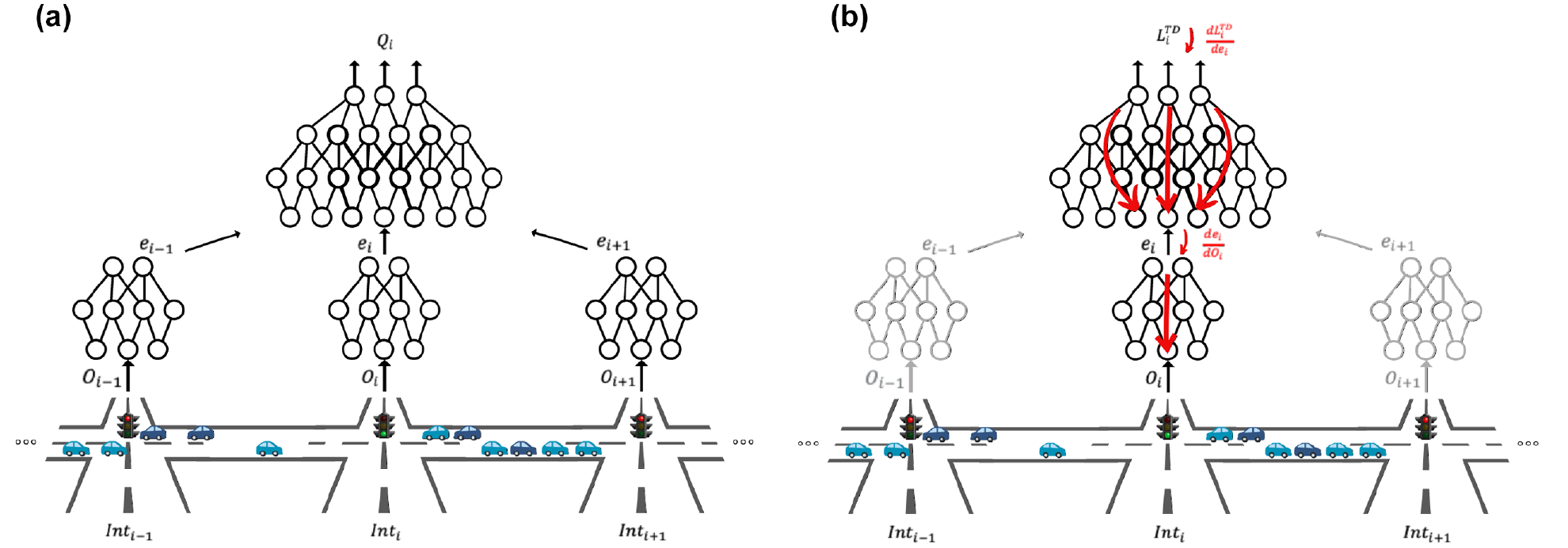
That is, the neighbors embedding are treated as constant inputs so they affect the Q-values (decisions and loss). Thus, the executor learns to consider them, but the embedding of a neighboring agent $j \in N_{i}$ is not affected by the calculation of agent $i$ . Thus, no transmission of gradients to the neighbors is required, and for agent $i$ , only the weights of its own executor and the local encoder are updated, as shown in Figure 1b.

Figure 1.

Forward and backward passes of the eMARLIN Q-network from the perspective of the ith intersection. The mappings $o_{i} \to e_{i}$ are trained locally across the whole intersection network. (a) Forward pass. Each immediate neighbor sends the encoded observation $e_{i \pm 1}$ (but not the raw observation $o_{i \pm 1}$ ) to intersection $i$ for the calculating the $Q_{i}$ vector. (b) Backward pass. Only the $o_{i} \to e_{i}$ mapping and the upper head of the network are being updated by back-propagation

Approach Motivation

A simple scenario motivated our work. It is possible that at a specific time, two intersections, one in the middle of the network and one close to the border, may obtain the same set of self and neighbors observations. Yet, it is clear their roles in the larger scheme are different. They are affected differently by what happens in the network and have different impacts on congestion. So, it is clear some information is missing in the raw observation of the network’s topology and the intersections’ role. The proposed learned embedding approach was meant to capture at least part of that information and use it for decision making. Furthermore, we considered the following properties during the design of our method:

Learning stability and reliability—fast convergence rate with consistent results.

Architectural simplicity—minimal amount of concurrently learning components, which affect each other’s performances.

Scalability—in both the number of intersections and the complexity of the phasing scheme (the cardinality of the action space).

Computational and communication lightness—not posing too heavy a burden on the communication network and lighter amount of computation than existing methods, allowing for lighter controllers that cannot handle multiple large neural networks.

Experiments

Here, we perform empirical experiments to test our method. We evaluate our method on two types of scenarios, synthetic and real world, each with unique properties, both in simulation. We compare our results to several baselines and state-of-the-art methods in the field and show the validity of our approach. All experiments are conducted on a server equipped with an AMD Ryzen 3990X CPU and 256 GB RAM.

Test Scenarios

Synthetic Grid Networks

We build synthetic grid networks of different scales in the Simulation of Urban MObility (SUMO) simulator ( 31 ). All intersections in the grid networks are signalized and controlled by external agents. Each of them have four single-lane approaches, four straight movements (no left, right, or U turns), and two phases (NS-through, EW-through). Each of the intersections uses a FPS (the single permitted phase transition is to the other phase). All approaches are classified as major approaches. The intersections are 300–1,500 m away from each other, depending on the specific scenario, as shown in Figure 2. All source and sink sections are 1,000 m long. The traffic demand is generated randomly with a time-varying probability on each of the source sections. The probability of spawning a vehicle per second on each of the source sections is sampled every 20 s from approach-dependent Gaussian distributions, as shown in Table 1. In all synthetic scenarios, horizontal origin–destination pairs are treated as corridors and are assigned higher demand compared with the vertical ones. The U.S. Department of Transportation Federal Highway Administration suggests a common range of saturation flow rate of 1,500–2,000 vehicles per hour per lane ( 32 ). Therefore, our synthetic networks cover a variety of traffic volume settings. We also test different algorithms on a time-varying environment, which is the Toronto network that covers light to medium traffic in a 4 h demand profile, to be discussed below.

Figure 2.

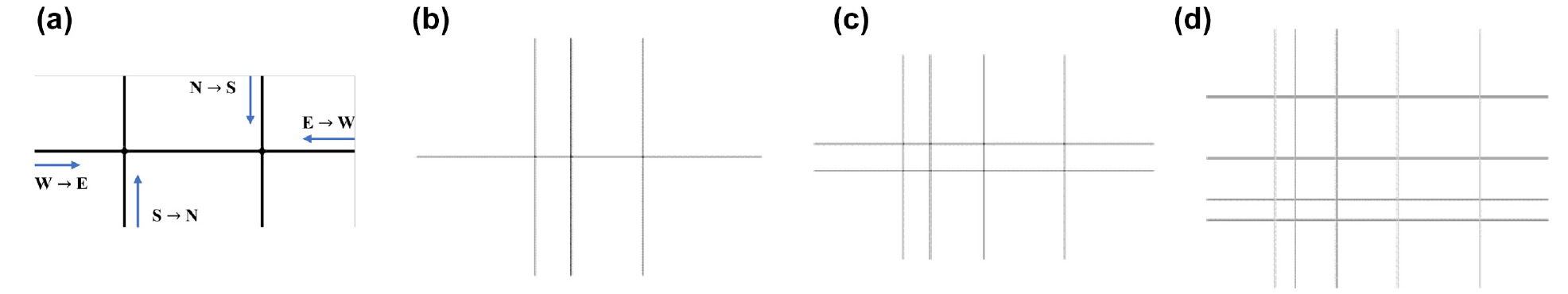
Illustration of synthetic grid networks modeled in Simulation of Urban MObility (SUMO): (a) Benchmark 0, 1 × 2; (b) Benchmark 1, 1 × 3; (c) Benchmark 2, 2 × 4; and (d) Benchmark 3, 4 × 5.

Table 1.

Synthetic Grid Network Traffic Demands

Scenario	Demand level	W→E	E→W	N→S	S→N
Benchmark 0, $1 \times 2$	Light	A platoon of 6 per 20 s	0	0	0
Benchmark 1, $1 \times 3$	Undersaturated	$N (0.4, 0.1)$	$N (0.04, 0.02)$	$N (0.04, 0.02)$	$N (0.04, 0.02)$
Benchmark 2, $2 \times 4$	Saturated	$N (0.4, 0.1)$	$N (0.4, 0.1)$	$N (0.1, 0.05)$	$N (0.1, 0.05)$
Benchmark 3, $4 \times 5$	Undersaturated	$N (0.3, 0.1)$	$N (0.3, 0.1)$	$N (0.1, 0.05)$	$N (0.1, 0.05)$

Note: W = west; E = east; N = north; S = south.

Toronto Network

We model a neighborhood of the intersection of Yonge Street and Steeles Avenue in Toronto, Canada, in the Aimsun simulator ( 33 ) (Figure 3). The network geometry is manually traced from a reference satellite image in the UTM-17 coordinate system. The modeled neighborhood consists of eight signalized intersections: Yonge–Steeles is an intersection of two major arterials, while the remaining seven intersections are intersections of a major arterial and a minor road. The distances between the signalized intersections vary between approximately 150 and 450 m.

Figure 3.

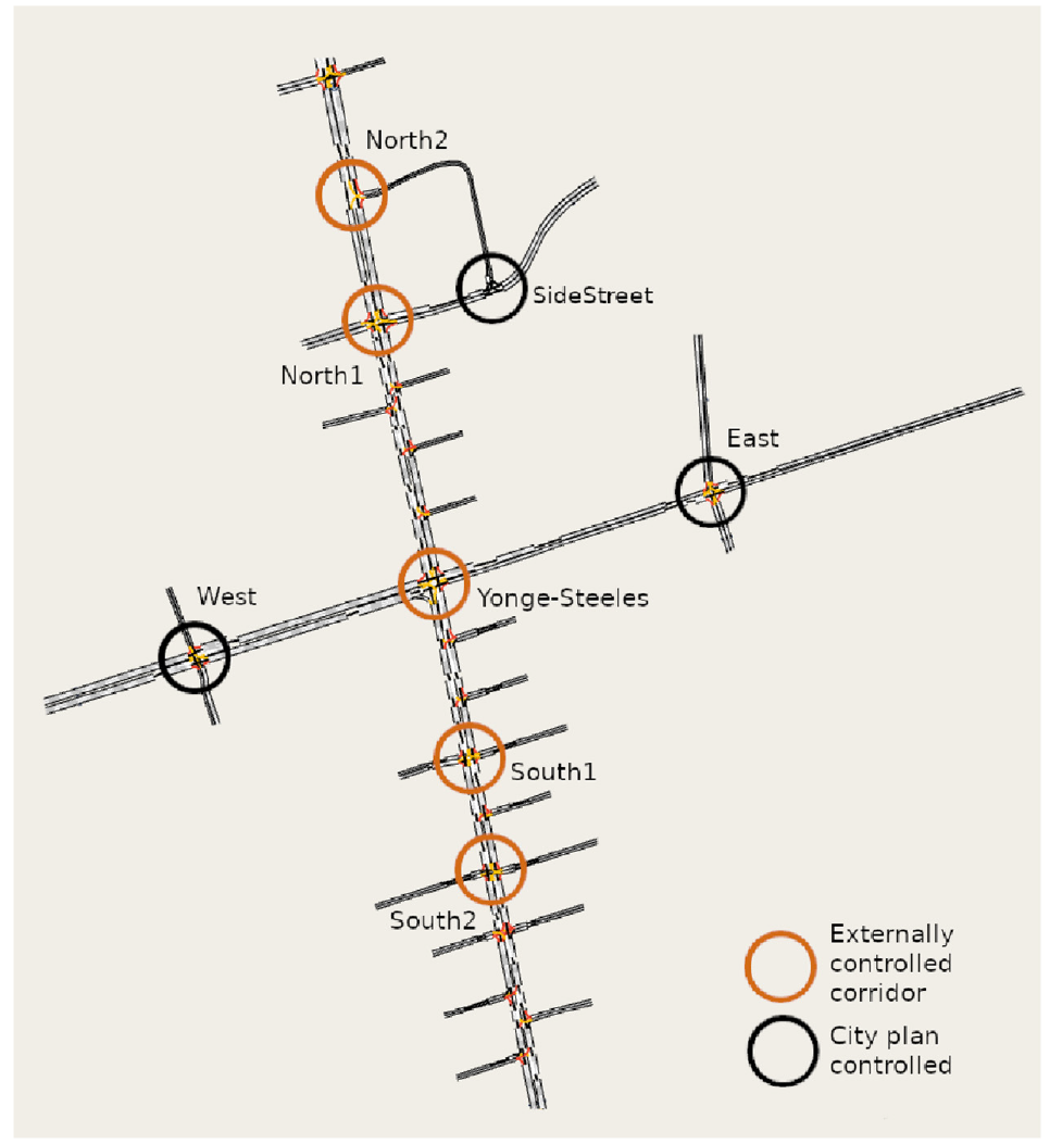
The Toronto network, with the signalized intersections circled and labeled.

The city signal timing plans (obtained from the city of Toronto) follow the standard NEMA phasing diagram, with semi-actuated control ( 4 ). The major through phases have a fixed duration and cannot be skipped, while the minor through phases and all phases that include a protected left turn are callable and extendable by loop detectors.

When evaluating eMARLIN, five intersections along Yonge Street (a north–south direction corridor) are controlled by external agents, and the remaining three intersections follow the city signal timing plans (Figure 4). The phasing scheme of the external agents is a CVPS, with a phase transition permitted in the phasing scheme if and only if the phase transition is possible under the city plan. This ensures a fair comparison of the RL controllers with the city plan.

Figure 4.

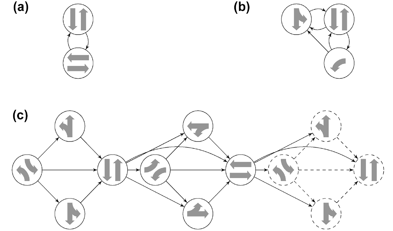
Constrained variable phasing schemes used in the test scenarios. Although not indicated in the figures, left turns are always permitted on through movements (when present), and right turns are always permitted (when present): (a) phasing scheme used for the synthetic grid networks, (b) phasing scheme used for the North2 intersection, which is a three-legged major-minor intersection, and (c) phasing scheme used for the Yonge–Steeles intersection. The leftmost four phases are duplicated on the right (the dashed nodes) to make the graph drawing clearer. The phasing scheme used for the remaining intersections (North1, South1, and South2) is similar, except the transitions from the North–South through phase to the other three North–South phases become permitted (North–South being the major and East–West the minor direction at these intersections, the East–West phases may be skipped by the controller).

The scenario traffic demand spans the morning peak period of 6–10 a.m. The demand is calibrated in several steps. First, the results of the 2016 Transportation Tomorrow Survey (TTS) ( 34 ) (origin–destination matrices between traffic analysis zones) are used to create the demand of a larger hybrid mesoscopic-microscopic model of the Greater Toronto and Hamilton Area (GTHA). The TTS traffic analysis zones that intersect our smaller subnetwork are kept as origins and destinations, each incoming link into the subnetwork gets assigned a new origin, and each outgoing link gets assigned a new destination. The incoming vehicle origin–destination pairs are accumulated in 15 min intervals from a simulation of the larger GTHA network. Then, the resulting origin–destination counts are adjusted using the techniques described in Aimsun ( 33 ) (“Integrating Macro, Meso, Micro, and Hybrid Simulations” tutorial), using turning movement counts at the subnetwork intersections (which are publicly available from the city of Toronto, accumulated in 15 min intervals). The turning movement counts of the final calibrated demand are a good fit to the city turning movement counts; the linear regression coefficient of determination (R²) is equal to 0.933.

Compared Baselines

We compare the proposed method to the following baselines (see also Figures 5 and 6):

City plan (Toronto network only): a standard NEMA phasing diagram with semi-actuated control activated ( 4 ).

MaxPressure ( 35 ): a decentralized heuristic method that greedily assigns right of way to the phase with the highest pressure.

PressLight ( 36 ): a decentralized DRL method that learns to minimize intersection pressure to balance queues in a traffic network.

Independent DQN (iDQN) ( 30 ): separate DQN agents for each of the controlled intersections without parameter sharing or any form of observation sharing.

iDQN-shareObs: iDQN agents taking one-hop neighbors’ observation as additional inputs.

Deep MARLIN ( 22 ): the DRL variant of MARLIN.

Note that different agents may operate on different state spaces. Specifically, iDQN-shareObs, Deep MARLIN, and eMARLIN consider the combination of the local observation space and all neighboring observation spaces as the state space for an agent. Conversely, Max-pressure defines the state space as the queue counts on all incoming and outgoing lanes. Additionally, PressLight defines the state space as the traffic status on all partitioned incoming and outgoing lanes, without any limitations with regard to detection ranges. We reproduce PressLight according to the description in the original paper. It uses the a variation of the pressure metric (based on vehicle counts rather than queued vehicle counts) as reward function.

Figure 5.

Forward pass for independent Deep Q-Network (iDQN) and iDQN-shareObs from the perspective of the $i$ th intersection. (a) iDQN. The Q-Network of the $i$ th intersection receives the observation $o_{i}$ only. (b) iDQN-shareObs. The Q-Network of the $i$ th intersection receives the observation $o_{i}$ , as well as the observations $o_{j}, j \in N_{i}$ of $i$ th one-hop neighborhood.

Figure 6.

Forward and backward passes for Deep-MARLIN from the perspective of the $i$ th intersection. (a) Forward pass. An ensemble of policy estimators and partial Q-networks, one of both for each neighbor $j \in N_{i}$ calculate the action probability of $a_{j}$ and the joint Q value $Q_{i}^{j} \in R^{| A_{i} | \times | A_{j} |}$ with regard to $o_{i}, o_{j}$ , respectively. The outputs are multiplied and summed in a majority voting-like mechanism to calculate the final $Q_{i}$ value. (b) Backward pass. The temporal difference (TD) error is used to calculate the gradients for the Q-networks. The policy estimation networks are trained with the cross-entropy loss in a supervised manner, according the neighbor’s actual taken action. Both types of networks are synchronously updated in each training step.

Evaluation Metrics

We evaluate the algorithm performance with a few metrics:

Episodic total delay (stopped time): the total time vehicles driving below the threshold speed (2 m/s) within all controlled intersections’ detection range (300 m).

Episodic average delay (AD): the average delay (stopped time) over all vehicles that have finished their trips.

Episodic average travel time (ATT): the average travel time over all vehicles that have finished their trips.

Training time: the world-clock time spent for finishing certain steps of training.

Neural Network Configuration

The observations are normalized before being input into a neural network. Vehicle counts (both queue and total counts on each lane) are normalized by passing them through the $\arctan$ function, which is a strictly increasing function $R \to (- π / 2, π / 2)$ . Note that this normalization is not applied for PressLight as it requires the raw observation. The size of neural networks of each RL algorithm is designed according to the searching space with respect to each scenario. Multiple configurations are evaluated. Table 2 presents the set of hyper-parameters that give the best results.

Table 2.

Neural Network Configurations for Reinforcement Learning Algorithms

Method	Hyper-parameter	Synthetic networks	Toronto network
iDQN	Q-network layer size	$[32, 32, 8]$	$[64, 64, 32]$
iDQN-shareObs	Q-network layer size	$[100, 100, 50]$	$[200, 200, 200, 100]$
Deep MARLIN	Partial-Q-network layer size	$[64, 32, 8]$	$[128, 128, 128]$
	Policy-estimator layer size	$[32, 32, 8]$	$[64, 64, 32]$
eMARLIN	Encoder layer size	$[32, 16]$	$[64, 64, 32]$
	Q-network layer size (per embedding)	$[16, 8]$	$[64, 32]$
PressLight	Q-network layer size	$[32, 32, 8]$	$[64, 64, 32]$

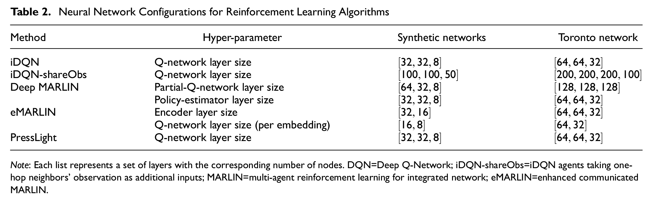
Note: Each list represents a set of layers with the corresponding number of nodes. DQN=Deep Q-Network; iDQN-shareObs=iDQN agents taking one-hop neighbors’ observation as additional inputs; MARLIN=multi-agent reinforcement learning for integrated network; eMARLIN=enhanced communicated MARLIN.

Results

Synthetic Grid Networks

With synthetic grid networks, we evaluate the coordination capability and the scalability of the proposed method. The results are shown in Table 3. We assign synthetic benchmark environments with high traffic volume to examine the capability of long-term planning. For a fair comparison across different experiments, we fix the seed for sampling vehicle-spawning probabilities during the evaluation stage. The proposed eMARLIN outperforms the iDQN consistently over scenarios with different scales under different demand levels, which indicates the positive effect of the information propagation mechanism. On the other hand, eMARLIN gives competitive results compared with deep MARLIN while having a lighter structure and lower computational requirements, as indicated by the running time of finishing $200, 000$ steps of training. iDQN-shareObs, with a heavy structure, requires neighbor observation as input but is not able to utilize it efficiently. Moreover, as the scale of the traffic network increases, from benchmark 1 to benchmark 3, eMARLIN shows a delay reduction with a similar margin (around 11%–16%), demonstrating the scalability of eMARLIN with respect to the traffic network scale.

Table 3.

Performance Comparison of all Methods on Synthetic Grid Networks

Scenario	Method	Total Pressure	Total delay (s)	AD (s)	ATT (s)	Running time (min)
BM 0 $1 \times 2$	MaxPressure	79.5	242.2	1.3	87.5	na
	PressLight	47.8	1,221.6	6.8	100.6	39.1
	iDQN	na	0.0	0.0	83.2	30.1
	iDQN-shareObs	na	0.0	0.0	82.2	44.3
	Deep MARLIN	na	0.0	0.0	82.3	64.5
	eMARLIN	na	0.0	0.0	82.2	48.5
BM 1 $1 \times 3$	MaxPressure	341.1	15,887.4	17.3	144.3	na
	PressLight	165.8	6,854.7	9.3	119.0	69.4
	iDQN	na	7,769.9	10.4	121.8	59.1
	iDQN-shareObs	na	7,436.8	10.6	122.0	74.3
	Deep MARLIN	na	6,832.3	9.7	120.6	108.2
	eMARLIN	na	6,532.1	9.7	119.9	82.6
BM 2 $2 \times 4$	MaxPressure	2,174.2	143,245.3	42.1	215.0	na
	PressLight	1,715.1	133,551.7	40.8	200.6	215.0
	iDQN	na	159,298.9	46.4	205.7	207.6
	iDQN-shareObs	na	147,988.0	42.1	205.7	291.9
	Deep MARLIN	na	138,051.6	40.4	204.2	472.7
	eMARLIN	na	134,249.9	39.6	201.6	302.9
BM 3 $4 \times 5$	MaxPressure	2,955.5	144,169.1	35.0	255.7	na
	PressLight	1,843.9	89,650.0	23.4	227.5	471.5
	iDQN	na	93,989.5	24.6	231.5	383.5
	iDQN-shareObs	na	95,172.5	25.3	234.9	580.1
	Deep MARLIN	na	76,720.4	20.4	227.4	1092.7
	eMARLIN	na	80,939.7	20.6	227.2	619.9

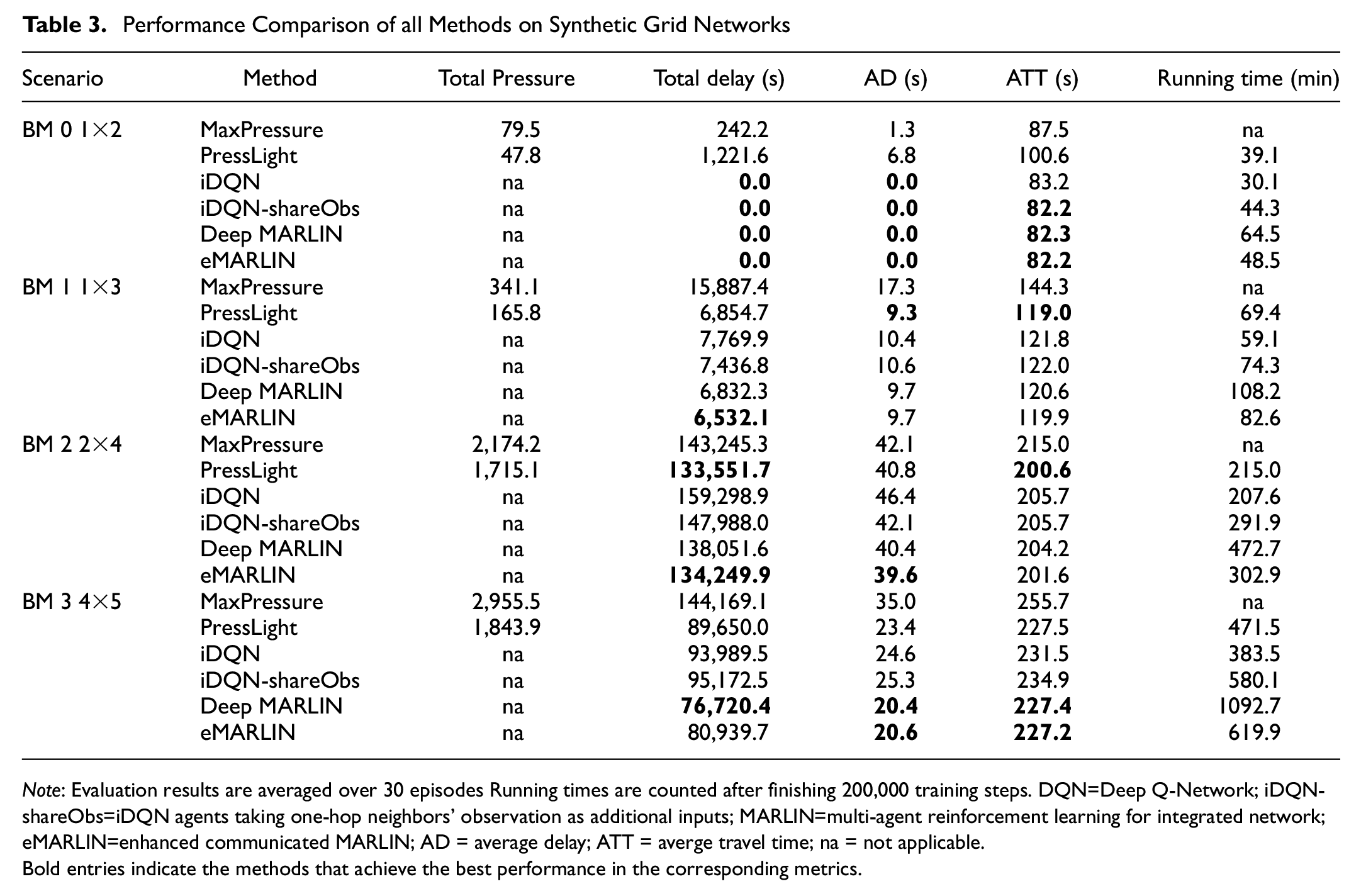
Note: Evaluation results are averaged over 30 episodes Running times are counted after finishing 200,000 training steps. DQN=Deep Q-Network; iDQN-shareObs=iDQN agents taking one-hop neighbors’ observation as additional inputs; MARLIN=multi-agent reinforcement learning for integrated network; eMARLIN=enhanced communicated MARLIN; AD = average delay; ATT = averge travel time; na = not applicable.

Bold entries indicate the methods that achieve the best performance in the corresponding metrics.

As for pressure-based methods, there is a clear trend in the results. PressLight works better under heavy traffic demand but suffers in light scenarios. Specifically, in benchmark $2$ , which has the heaviest demand, by optimizing intersection pressure, PressLight achieves the highest scores across most metrics. However, it fails to compete with other methods in benchmark $0$ , the simplest scenario. This means that the vehicle count variant of pressure is not always positively related to other traffic metrics. For example, in benchmark $0$ , even though PressLight tries to optimize the intersection pressure, its performance is inferior to the max-pressure policy.

Toronto Network

Table 4 summarizes the experiment results under a realistic environment, the Toronto network. It shows that eMARLIN outperforms all baseline methods by a visible margin: $48.7 %$ of delay time saving compared with the city plan, and $13.7 %$ of delay time saving compared with iDQN. Specifically, eMARLIN agents obtain the lowest local delays on three out of five intersections while getting lower local delays across all intersections compared with iDQN. This again suggests the effectiveness of the proposed information propagation mechanism with respect to enabling better coordination. Compared with the city plan, eMARLIN performs worse on the intersection South $1$ but compensates for such a deterioration by the huge delay time saving on neighboring intersections.

Table 4.

Performance Comparison on the Toronto Test Bed.

Method	North2	North1	Yonge–Steeles	South1	South2	Sum
City plan	2,120	77,222	465,500	6,091	49,965	600,898
PressLight	23,590	101,091	276,824	60,180	115,070	576,755
PressLight-center-only	na	na	199,443	na	na	na
iDQN	7,169	61,029	197,544	40,999	50,288	357,029
iDQN-shareObs	4,566	57,818	237,872	9,417	48,481	358,154
Deep MARLIN	1,261	54,790	187,103	5,982	48,719	297,855
eMARLIN	1,027	60,800	174,464	8,174	48,170	292,635

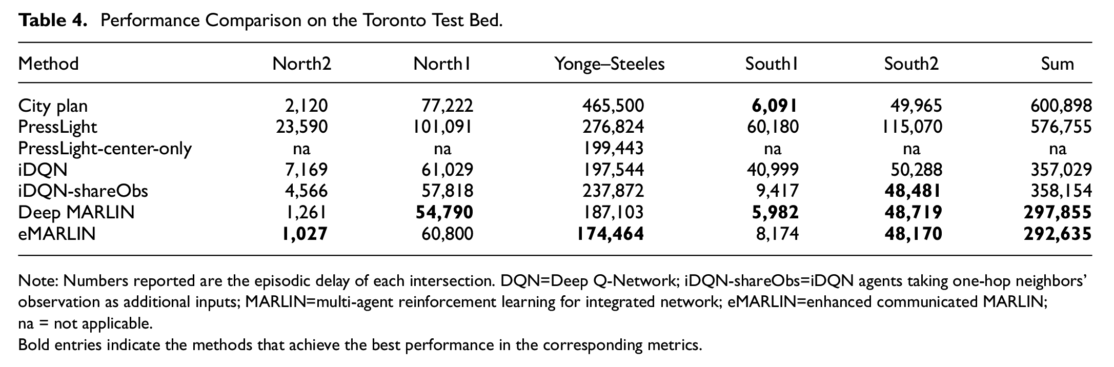
Note: Numbers reported are the episodic delay of each intersection. DQN=Deep Q-Network; iDQN-shareObs=iDQN agents taking one-hop neighbors’ observation as additional inputs; MARLIN=multi-agent reinforcement learning for integrated network; eMARLIN=enhanced communicated MARLIN; na = not applicable.

Bold entries indicate the methods that achieve the best performance in the corresponding metrics.

The max-pressure policy is not tested under the Toronto network, since it requires greedy change to the phase with the largest pressure, which implies a VPS phasing scheme. Following NEMA constraints, we adhere to the CVPS phasing scheme. Thus, the comparison of max-pressure to the other controllers is incompatible.

Although PressLight agents converge on the pressure reward, since the pressure is not always positively correlated with other traffic metrics, as we have shown in the previous result discussion, PressLight fails to learn a proper policy on the Toronto network, which has a light-to-medium volume and time-varying demand profile. In particular, PressLight performs significantly worse than the city plan at the four peripheral intersections, since there are light but dominating north-/southbound flows, which are similar to benchmark $0$ . In addition, to demonstrate that PressLight can actually perform well under a scenario that is more suitable to its design of queue balancing, we trained a single agent on the center Yonge–Steeles intersection and left the other four intersections using the City Plan. The result is labeled as “PressLight-center-only” in Table 4. Performance of the central agent in row “PressLight” deteriorates from “PressLight-center-only” as expected. That is because as peripheral intersections are also controlled by learning agents rather than a fixed policy, the nonstationarity introduced across agents makes their learning more difficult. It is worth noting that DQN agents also suffer from a similar deterioration phenomenon.

Last, we present the TD loss of all approaches as a measure of learning stability and the convergence rate in Figure 7. The results are given for BM1 and BM2 as representative scenarios, where all methods showed the ability to cope and learn meaningful policies. Results are presented consistently for the most central intersection only. As expected, iDQN as an isolated method learns fast, but the loss is not stable. iDQN-shareObs is able to learn something useful, but once again, the heavy architecture results in a slow learning rate. Deep-MARLIN, the heaviest of them all, requires the policy to stabilize before the Q part can converge and exhibits the slowest learning. eMARLIN performs as desired. It learns fast, and the TD loss is quite stable at a low value.

Figure 7.

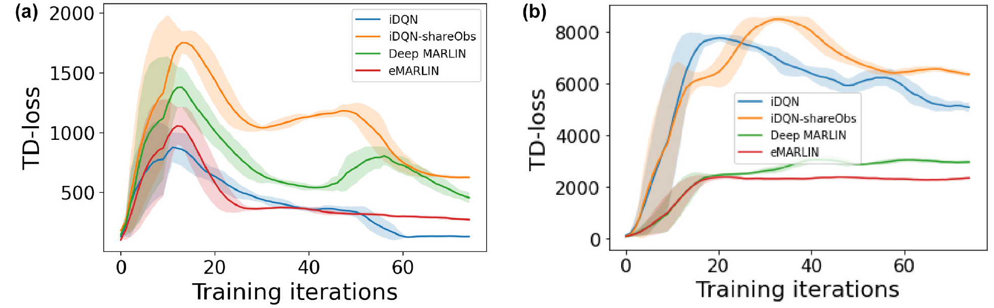
Illustration of the training progress of different methods with respect to the temporal difference (TD) losses: (a) Benchmark 1 TD loss and (b) Benchmark 2 TD loss.

Discussion and Conclusion

We have addressed the problem of reducing traffic delays in urban traffic networks. A decentralized learning method has been presented based on the DQN algorithm in a multi-agent reinforcement learning setting. Our method decouples the Q-network into two components: encoder and executor. Intersections encode their local raw observations into an embedding latent space, with corresponding encoders, and then share this embedding with their one-hop neighbors. The intersections’ executors play the role of Q-networks, taking self and neighbors’ embedding as input and making decisions. Encoders are jointly trained with executors within each private intersection such that no gradient back-propagation across agents is required. Such a strategy ensures the minimum communication bandwidth requirement after deployment, while maintaining the capability of conducting policy updates online. Empirical experiments demonstrate the strong performance and learning stability of the proposed method compared with related decentralized learning algorithms. Future studies should investigate the information transferred within the embedding, and whether information of longer than one-hop distance is being propagated by the embedding.

Footnotes

Author Contributions

The authors confirm contribution to the paper as follows: study conception and design: Xiaoyu Wang, Ayal Taitler, Ilia Smirnov, Scott Sanner, and Baher Abdulhai; data collection: Ilia Smirnov; analysis and interpretation of results: Xiaoyu Wang; draft manuscript preparation: Xiaoyu Wang, Ayal Taitler, and Ilia Smirnov. All authors reviewed the results and approved the final version of the manuscript.

Declaration of Conflicting Interests

The author(s) declared no potential conflicts of interest with respect to the research, authorship, and/or publication of this article.

Funding

The author(s) received no financial support for the research, authorship, and/or publication of this article.

ORCID iDs

Xiaoyu Wang,

Ayal Taitler,

Scott Sanner,

Baher Abdulhai,

References

Grote

Williams

Preston

Kemp

Including Congestion Effects in Urban Road Traffic CO₂ Emissions Modelling: Do Local Government Authorities have the Right Options?

Transportation Research Part D: Transport and Environment, Vol. 43, 2016, pp. 95–106.

Fan

CO₂ Emissions and Expansion of Railway, Road, Airline and In-Land Waterway Networks Over the 1985–2013 Period in China: A Time Series Analysis. Transportation Research Part D: Transport and Environment, Vol. 57, 2017, pp. 130–140.

Webster

. Traffic Signal Settings. Road Research Technique Paper No. 39. Road Research Laboratory, London, 1958.

FHWA. Appendix F: Actuated Signal Control. In: Traffic Analysis Toolbox Volume IV: Guidelines for Applying CORSIM Microsimulation Modeling Software ( Holm

Tomich

Sloboden

Lowrance

, eds.), U.S. Department of Transportation Federal Highway Administration, Washington, D.C., 2007.

El-Tantawy

Abdulhai

Abdelgawad

Multiagent Reinforcement Learning for Integrated Network of Adaptive Traffic Signal Controllers (MARLIN-ATSC): Methodology and Large-Scale Application on Downtown Toronto. IEEE Transactions on Intelligent Transportation Systems, Vol. 14, No. 3, 2013, pp. 1140–1150.

Guilliard

Sanner

Trevizan

F. W.

Williams

B. C.

Nonhomogeneous Time Mixed Integer Linear Programming Formulation for Traffic Signal Control. Transport Research Record: Journal of the Transport Research Board, 2016. 2595: 128–138.

Little

J. D.

Kelson

M. D.

Gartner

N. H.

MAXBAND: A Program for Setting Signals on Arteries and Triangular Networks. Transportation Research Record: Journal of the Transportation Research Board, 1981. 795: 40–46.

Gartner

N. H.

Assmann

S. F.

Lasaga

Hous

D. L.

MULTIBAND—A Variable-Bandwidth Arterial Progression Scheme. Transportation Research Record: Journal of the Transportation Research Board, 1990. 1287: 212–222.

Robertson

D. I.

TRANSYT: A Traffic Network Study Tool. RRL Report LR 253. Road Research Laboratory, Crowthorne, U.K., 1969.

10.

Shalaby

W. X.

Corby

Wong

Zhou

Chapter 16: Transit Signal Priority: Research and Practice Review and Future Needs. Edward Elgar Publishing, Cheltenham, U.K., 2021.

11.

Hunt

Robertson

Bretherton

Winton

SCOOT-A Traffic Responsive Method of Coordinating Signals. LR-1014. Transport and Road Research Laboratory Report, Crawthorne, U.K., 1981.

12.

Sims

Dobinson

SCAT the Sydney Coordinated Adaptive Traffic System: Philosophy and Benefits. Proc., International Symposium on Traffic Control Systems, Berkeley, CA, Vol. 2, 1979.

13.

Smith

S. F.

Barlow

G. J.

Xie

X. F.

Rubinstein

Z. B.

Smart Urban Signal Networks: Initial Application of the Surtrac Adaptive Traffic Signal Control System. Proc., 23rd International Conference on Automated Planning and Scheduling, Rome, Italy, 2013.

14.

Silver

Huang

Maddison

C. J.

Guez

Sifre

Van Den Driessche

Schrittwieser

, et al. Mastering the Game of Go with Deep Neural Networks and Tree Search. Nature, Vol. 529, No. 7587, 2016, pp. 484–489.

15.

Chu

Wang

Codecà

Multi-Agent Deep Reinforcement Learning for Large-Scale Traffic Signal Control. IEEE Transactions on Intelligent Transportation Systems, Vol. 21, No. 3, 2019, pp. 1086–1095.

16.

Liang

Fang

Zhong

OAM: An Option-Action Reinforcement Learning Framework for Universal Multi-Intersection Control. Proceedings of the AAAI Conference on Artificial Intelligence, Vol. 36, No. 4, 2022. pp. 4550–4558.

17.

Alizadeh Shabestray

S. M.

Abdulhai

Multimodal iNtelligent Deep (MiND) Traffic Signal Controller. Proc., IEEE Intelligent Transportation Systems Conference (ITSC), Auckland, New Zealand, IEEE, NY, 2019. pp. 4532–4539.

18.

Wei

Zhang

Zheng

Zang

Chen

Zhang

Zhu

CoLight: Learning Network-Level Cooperation for Traffic Signal Control. Proc., 28th ACM International Conference on Information and Knowledge Management, Beijing, China, Association for Computing Machinery, New York, 2019, pp. 1913–1922.

19.

Oroojlooy

Nazari

Hajinezhad

Silva

Attendlight: Universal Attention-Based Reinforcement Learning Model for Traffic Signal Control. Advances in Neural Information Processing Systems, Vol. 33, 2020, pp. 4079–4090.

20.

Devailly

F. X.

Larocque

Charlin

IG-RL: Inductive Graph Reinforcement Learning for Massive-Scale Traffic Signal Control. IEEE Transactions on Intelligent Transportation Systems, Vol. 23, No. 7, 2022, pp. 7496–7507.

21.

Jaggi

Wang

Carrara

Sanner

Abdulhai

Microscopic Model-Based RL Approaches for Traffic Signal Control Generalize Better than Model-Free RL Approaches. Proc., IEEE International Intelligent Transportation Systems Conference (ITSC), Indianapolis, IN, IEEE, NY, 2021. pp. 2525–2532.

22.

Klöckner

Klose

deep-MARLIN: Using Deep Multi-Agent Reinforcement Learning for Adaptive Traffic Light Control. Proc., 3rd International Conference on Applications of Intelligent Systems, Las Palmas de Gran Canaria, Spain, Association for Computing Machinery, New York, 2020, pp. 1–6.

23.

Zhou

Chen

Liu

Braud

Hui

Kangasharju

DRLE: Decentralized Reinforcement Learning at the Edge for Traffic Light Control in the IoV. IEEE Transactions on Intelligent Transportation Systems, Vol. 22, No. 4, 2021, pp. 2262–2273.

24.

Wang

Zhu

Zhou

Luo

Zhang

GAN and Multi-Agent DRL Based Decentralized Traffic Light Signal Control. IEEE Transactions on Vehicular Technology, Vol. 71, No. 2, 2022, pp. 1333–1348.

25.

Puterman

M. L.

Markov Decision Processes: Discrete Stochastic Dynamic Programming. John Wiley & Sons, Hoboken, NJ, 2014.

26.

Sutton

R. S.

Barto

A. G.

Reinforcement Learning: An Introduction. A Bradford Book, Cambridge, MA, 2018.

27.

Bernstein

D. S.

Givan

Immerman

Zilberstein

The Complexity of Decentralized Control of Markov Decision Processes. Mathematics of Operations Research, Vol. 27, No. 4, 2002, pp. 819–840.

28.

Papadimitriou

C. H.

Tsitsiklis

J. N.

The Complexity of Markov Decision Processes. Mathematics of Operations Research, Vol. 12, No. 3, 1987, pp. 441–450.

29.

Chen

Wei

Zheng

Yang

Xiong

. Toward a thousand Lights: Decentralized Deep Reinforcement Learning for Large-Scale Traffic Signal Control. Proceedings of the AAAI Conference on Artificial Intelligence, Vol. 34, No. 4, 2020. pp. 3414–3421.

30.

Mnih

Kavukcuoglu

Silver

Graves

Antonoglou

Wierstra

Riedmiller

Playing Atari with Deep Reinforcement Learning. arXiv preprint arXiv:13125602, 2013.

31.

Lopez

P. A.

Behrisch

Bieker-Walz

Erdmann

Flötteröd

Y. P.

Hilbrich

Lücken

Rummel

Wagner

Wiessner

Microscopic Traffic Simulation Using SUMO. Proc., 21st International Conference on Intelligent Transportation Systems (ITSC), Maui, HI, IEEE, NY, 2018, pp. 2575–2582.

32.

FHWA. Operational and Safety Analysis. In: Traffic Signal Timing Manual ( Koonce

Rodegerdts

Lee

Quayle

Beaird

Braud

Bonneson

Tarnoff

Urbanik

, eds.), U.S. Department of Transportation Federal Highway Administration, Washington, D.C., 2005.

33.

Aimsun. Aimsun Next 22 User’s Manual. Barcelona, Spain, 2022. https://docs.aimsun.com/next/22.0.1/. Accessed July 3, 2023.

34.

University of Toronto Data Management Group. Transportation Tomorrow Survey 2016: Design and Conduct of the Survey. 2016. http://dmg.utoronto.ca/pdf/tts/2016/2016TTS_Conduct.pdf. Accessed July 30, 2022.

35.

Varaiya

The Max-Pressure Controller for Arbitrary Networks of Signalized Intersections. In: Advances in Dynamic Network Modeling in Complex Transportation Systems ( Ukkusuri

S. V.

Ozbay

, eds.), Springer, New York, 2013, pp. 27–66.

36.

Wei

Chen

Zheng

Gayah

Presslight: Learning Max Pressure Control to Coordinate Traffic Signals in Arterial Network. Proc., 25th ACM SIGKDD International Conference on Knowledge Discovery & Data Mining, Anchorage, AK, Association for Computing Machinery, New York, 2019, pp. 1290–1298.