Considering the Spatial Structure of the Road Network in Pavement Deterioration Modeling

Abstract

Pavement deterioration modeling is important in providing information with respect to the future state of the road network and in determining the needs of preventive maintenance or rehabilitation treatments. This research incorporated the spatial dependence of the road network into pavement deterioration modeling through a graph neural network (GNN). The key motivation of using a GNN for pavement performance modeling is the ability to easily and directly exploit the rich structural information in the network. This paper explored if considering the spatial structure of the road network will improve the prediction performance of the deterioration models. The data used in this research comprises a large pavement condition dataset with more than a half million observations taken from the Pavement Management Information System maintained by the Texas Department of Transportation. The promising comparison results indicate that pavement deterioration prediction models perform better when the spatial relationship is considered.

Keywords

data and data science deep learning infrastructure infrastructure management and system preservation pavement management systems pavement management

The spatial relationships between infrastructure facilities have been studied in the area of asset management by previous researchers. For example, Zou and Madanat ( 1 ) presented an approach to address pavement management decision problems at airports with multiple runways by considering functional dependence between runways. Atef and Moselhi ( 2 ) presented a framework to model spatially and functionally dependent assets. The developed model can be used to determine an asset's degree of connectivity with its neighbors. Another group of researchers studied the economic dependence of the road network structure. In those cases, often the cost of executing work on upholding many components’ integrity at the same time can be cheaper than doing the same work on individual components collectively. This includes the scenarios where doing any kind of maintenance work requires large amounts of setup and preparation work to be done in advance. Bernhardt et al. ( 3 ) noted that pavements are interconnected through geography, which implied the economies of scale in contracting long stretches of pavement for rehabilitation and the diseconomies of scale with respect to the disruption to users. Some other researchers have studied the failure dependence among infrastructure facilities or systems. For example, McDaniels et al. ( 4 ) developed an analytical framework to characterize infrastructure failure interdependencies. The authors studied how extreme events lead to failures of other spatially connected infrastructure systems, for example, given a major electrical power outage. Rahman et al. ( 5 ) used public domain failure reports to identify the origin of these failures and their propagation patterns. The authors studied historical records to determine the causes of infrastructure failures and the impact of failures in the spatial and temporal dimensions. Panzieri et al. ( 6 ) analyzed performance degradation induced by the spreading of failures to emphasize the most critical links existing among different critical infrastructure networks. Spatial dependency has also been taken into consideration in developing pavement deterioration models through recognizing similarities between adjacent sections. This is usually conducted through developing separate models for the pavement in different categories (climate, traffic, material). Despite these efforts in previous research, there is a lack of studies that take neighboring sections’ information into consideration when developing pavement deterioration models. It is possible that the prediction of a pavement section’s deterioration can be improved by taking into consideration neighboring sections’ condition information because they are all exposed to a set of common factors that make them fail, such as loading, operation, or environmental factors.

Recently, with the development of big data and artificial intelligence, deep learning models, primarily the convolutional neural network (CNN) and long short-term memory (LSTM), have received considerable attention in the pavement performance modeling area. Compared with traditional models, deep learning models are designed to make more accurate prediction results. For example, Lee et al. ( 7 ) developed a pavement deterioration prediction model based on a deep neural network (NN) and a recurrent neural network (RNN) with LSTM circuits. They found that the performance and accuracy of the LSTM model was superior. Choi and Do ( 8 ) predicted the deterioration of a road pavement by using monitoring data and a LSTM framework. The constructed algorithm predicted the pavement condition index (PCI) for each section of the road network for one year by learning from the time series data for the preceding 10 years. Hosseini et al. ( 9 ) developed deterioration models for the PCI as a function of time using two modeling approaches: the deep learning model of LSTM and individual regression models. A comparison was made between the two approaches and the results show that the LSTM model achieved a higher prediction accuracy over time for all different pavement types. Gao et al. ( 10 ) employed a deep learning-based deterioration model through a CNN-LSTM combined framework to detect if an maintenance and rehabilitation (M&R) treatment was applied to a pavement section during a given time period. Haddad et al. ( 11 ) used a deep NN for pavement rutting prediction. The predictive capability of the proposed model was compared to a multivariate linear regression (LR) model fitted using the same dataset. It was found that the deep NN rutting prediction model enhanced predictive power compared to commonly used models in the literature. Zhou et al. ( 12 ) also applied the LSTM model to predict an asphalt concrete (AC) pavement international roughness index (IRI), utilizing datasets extracted from the Long-Term Pavement Performance (LTPP) database. Gao et al. ( 13 ) introduced a convolutional graph neural network (GNN) for imputing missing pavement condition data in pavement management systems, outperforming standard machine learning models.

In this research, we investigated applying a special class of deep learning methods called the GNN for pavement deterioration modeling. The GNN is a class of deep learning methods designed to perform inference on data described by graphs. The objective of this research is to study if the prediction of a pavement section’s deterioration can be improved by taking neighboring sections’ condition information into consideration.

Methodology

The GNN is one of the fastest growing areas in deep learning. Its popularity lies in its strength to utilize the graph structure of data in a network format, such as transportation networks, social networks, and biology ( 14 ). Compared with traditional machine learning and deep learning models, the advantage of the GNN is that it is able to utilize the spatial relationship between data points and aggregate information through graph edges. In the case of the road network in this research, individual pavement sections are modeled as graph nodes, and the connections between the sections are modeled as graph edges. The way the GNN works is to create node embeddings where information of individual nodes is represented as low-dimensional vectors and the links (relationships between nodes) are maintained in the graph structure. With this setting, the model can be used for graph classification, node classification, or regression.

In this research, we used the Graph Sample and Aggregate (GraphSAGE) ( 15 ) model, which is one of the commonly used GNN models. GraphSAGE allows training large-scale networks with mini-batch setting, where the model learns a function that outputs node embeddings based on the neighborhood of a node rather than learning all of the node embeddings directly. This significantly limits the memory and time needed to train the model for large networks.

We define the road network as a graph $G (V, E)$ with $V$ representing nodes (pavement sections) and $E$ indicating the connections between them. The information (e.g., traffic, environment, pavement type) of a section $v$ is represented as the vector $x_{v}$ , and the complete set of node feature vectors as { $x_{v}$ , $\forall v \in V$ }. The number of graph layers, K, in the GraphSAGE model specifies the number of hops the information of each node can travel across the graph.

The message passing workflow of the GraphSAGE model mainly consists of two components, which are shown in Figure 1. The first component is neighborhood sampling of the input graph. The second component is aggregating information at each search depth. Using this message passing mechanism, the GNN is able to embed into each node information about its neighbors and then employ the embedded information to make predictions. A major difference between the GNN and other machine learning models is that the GNN can deal with variable sized graph inputs and other models cannot. For a standard machine learning model, adding neighbor information as extra features works only for a graph with a fixed number of neighbors for each node. The GNN can handle graphs whose nodes have variable numbers of neighbors.

Figure 1.

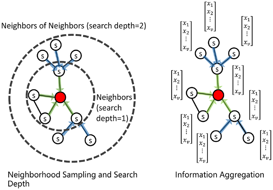
Neighborhood sampling and information aggregation of the Graph Sample and Aggregate model.

Once information is collected from neighboring nodes, a MEAN_k, $\forall k \in {1, \dots, K}$ , aggregate function is used to calculate the average information. For each node, the GraphSAGE model iteratively aggregates information from the node’s neighborhood, the node’s neighbors’ neighborhood, and so on. At the training, the aggregated information $h_{N (v)}^{k}$ of node $v$ at the $k$ th layer can be expressed as follows:

h_{N (v)}^{k} = MEA N_{k} ({h_{u}^{k - 1}, \forall u \in N (v)})

(1)

where $N (v)$ is the sampled neighborhood of node $v$ and $h_{u}^{k - 1}$ represents the embedding of node $u$ in the previous layer. The aggregated embeddings of the sampled neighborhood $h_{N (v)}^{k}$ are then concatenated with the nodes’ embeddings from the previous layer $h_{v}^{k - 1}$ . The node $v$ at the layer $k$ embedding can be calculated by applying the model’s trainable parameters, $W^{k}$ , and passing the result through a non-linear activation function $σ$ (e.g., a rectified linear unit [ReLU]):

h_{v}^{k} = σ (W^{k} \cdot h_{v}^{k - 1} \cup h_{N (v)}^{k})

(2)

The final embedding of node $v$ at the final layer $K$ is expressed as $z_{v}$ , as shown in Equation 3:

z_{v} = h_{v}^{K}, \forall v \in V

(3)

Case Study

Data Description

To demonstrate and evaluate the applicability of the proposed model, a case study was carried out using pavement condition inventory data (more than 110,000 data points each year) from the Texas Department of Transportation (TxDOT). The data used were collected from pavement sections (around 0.5 mi in length) across Texas between 2014 and 2018. Each pavement section is labeled with a unique reference marker, which was used to create the spatial relationships between a section and its neighbors in this research. If one section’s ending reference marker is the same as another section’s beginning reference marker, these two sections are considered connected and neighbors.

The variables used in this study contain key attributes of pavement condition observations and other related variables, as shown in Table 1. Although the initial condition right after a maintenance and rehabilitation treatment is usually used to model post-treatment deterioration, that information is not available in the dataset of this case study. For this reason, we did not create a variable indicating the post-treatment condition. Instead, we used annual inspected condition data where the average time between a treatment and the next inspection is around half a year.

Table 1.

Variables

Variables	Description
Pavement condition indicators	There were 12 condition indicators used in this case study. Detailed information about indicators can be found in Table 2.
Time since last treatment	The time difference in years between the last applied treatment and 2018.
Traffic	The current 18-kip ESAL value for the data collection section. Values are stored in thousands.
Road work records	Treatment types recorded by TxDOT. Detailed information about treatment types can be found in Table 3
Climatic regions	Climate zones based on temperature and precipitation
Type of pavement surface	ACP surface types based on the similarity of characteristics
Functional class	In Texas, highways are categorized into seven groups based on their function, and each group contains sub-groups ( 16 ).

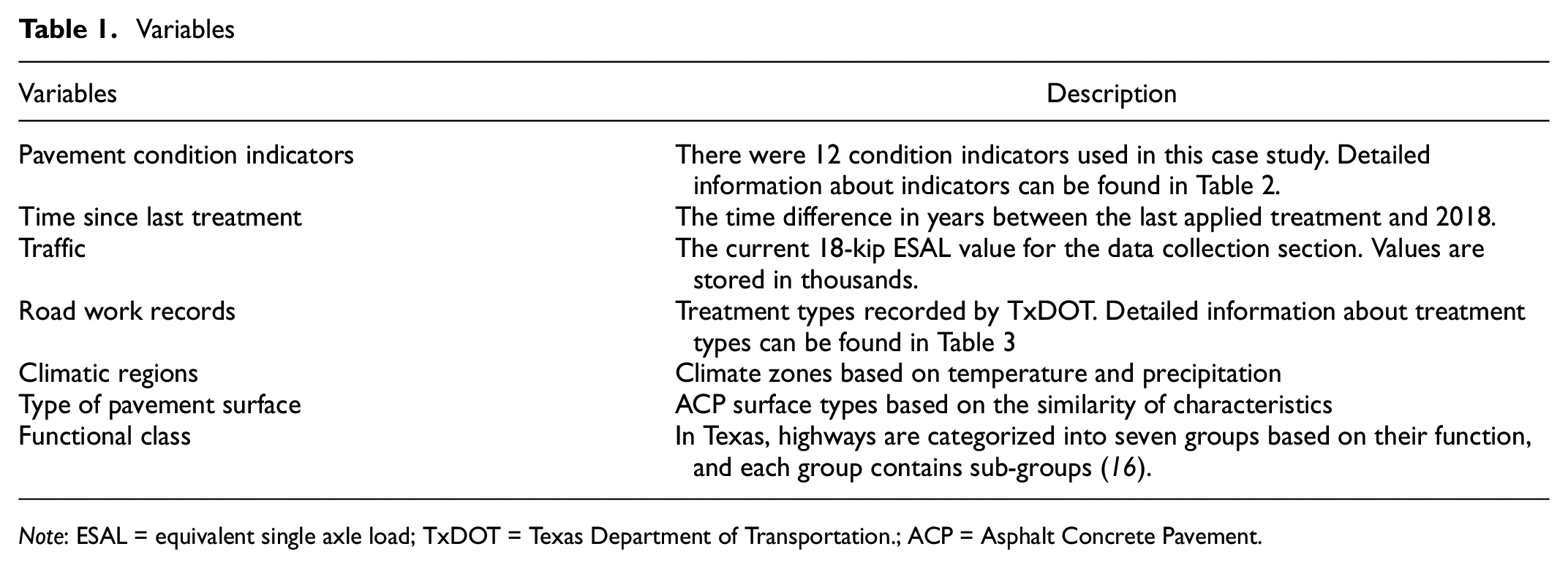
Note: ESAL = equivalent single axle load; TxDOT = Texas Department of Transportation.; ACP = Asphalt Concrete Pavement.

Condition Indicator

The condition variables include 12 flexible pavement condition indicators, which are shown in Table 2. The TxDOT pavement management system stores three scores that represent the general condition of a pavement ( 17 ). The distress score (DS) reflects the amount of visible surface deterioration of a pavement, with a range from 1 (the most distress) to 100 (the least distress). The ride score (RS) is a measure of the pavement’s roughness, ranging from 0.1 (the roughest) to 5.0 (the smoothest). The condition score (CS) represents the pavement’s overall condition with respect to both distress and ride quality, ranging from 1 (the worst condition) to 100 (the best condition). Other indicators include shallow rutting, deep rutting, patching, failures, block cracking, alligator cracking, longitudinal cracking, transverse cracking, and the IRI.

Table 2.

Pavement Condition Indicators

#	Condition indicator	Unit	Range
1	Shallow rutting (0.25–0.49 in. depth)	Percentage	0–100
2	Deep rutting (0.50–0.99 in. depth)	Percentage	0–100
3	Patching	Percentage	0–100
4	Failures	Quantity	$\geq 0$
5	Block cracking	Percentage	0–100
6	Alligator cracking	Percentage	0–100
7	Longitudinal cracking	Foot	$\geq 0$
8	Transverse cracking	Quantity	$\geq 0$
9	IRI	in./mi	$\geq 0$
10	Ride score	na	0–5
11	Distress score	na	0–100
12	Condition score	na	0–100

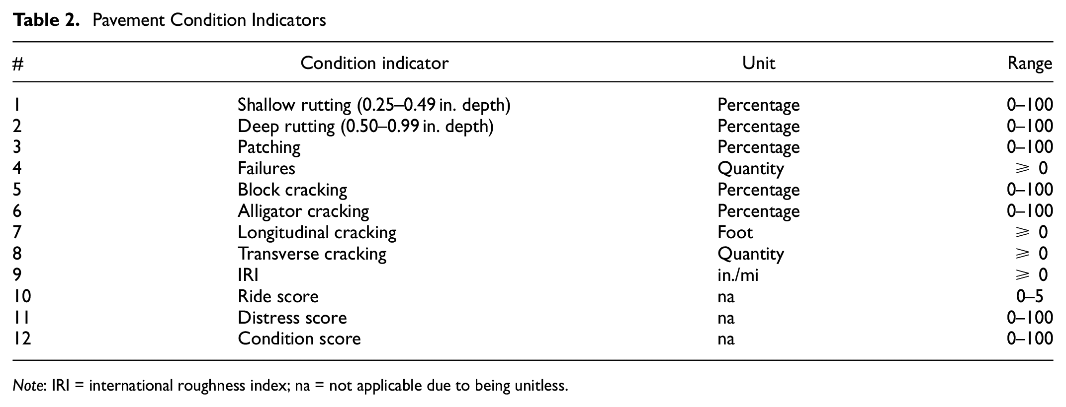
Note: IRI = international roughness index; na = not applicable due to being unitless.

Pavement Type

There are 10 different types of pavements in the TxDOT pavement management system. In this research, five asphalt pavement types (codes: 4, 5, 6, 9, and 10) were used (Figure 2). Code 4 represents thick AC (greater than 5.5 in.). Code 5 indicates medium thickness AC (2.5–5.5 in.). Code 6 represents thin AC (less than 2.5 in.). Code 9 represents overlaid and widened AC pavement. Code 10 represents thin surfaced flexible pavement (surface treatment or seal coat).

Figure 2.

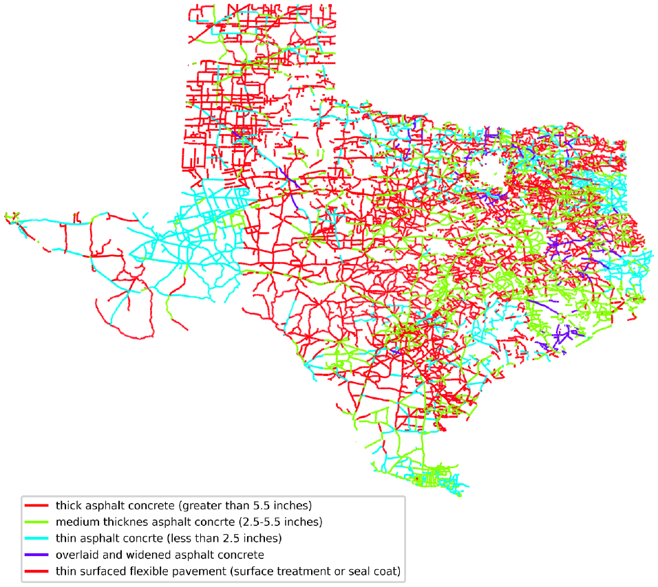
Map of the data used in this case study by different pavement types.

Functional Classification

In Texas, highways are categorized into different groups based on their function ( 17 ). In this case study, 19 different groups of highways are used. As shown in Figure 3, most of the highways fall into the groups of farm-to-market (FM), state highway (SH), U.S. highway (US), and interstate highway (IH), which correspond to more than 90% of all the records.

Figure 3.

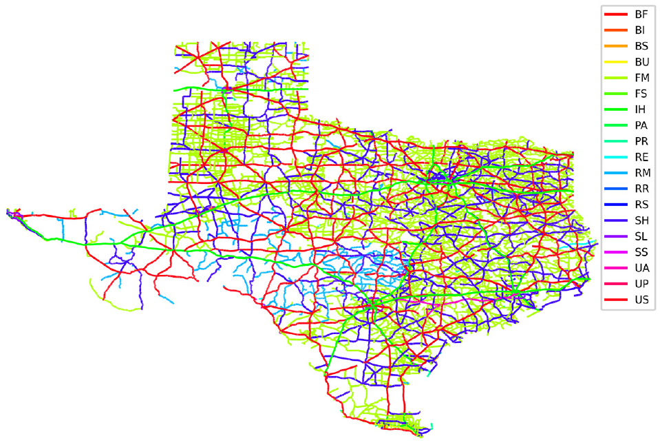
Map of the data used in this case study by different functional classes.Note: BF = Business Farm to Market Roads; BI = Business IH Highways; BS = Business State Highways; BU = Business US Highways; FM = Farm to Market Road; FS = Farm to Market Road Spurs; IH = Interstate Highway; PA = Principle Arterial Street System; PR = Park Road; RE = Recreational Road; RM = Ranch to Market Road; RR = Ranch Road; RS = Ranch to Market Road Spur; SH = State Highway; SL = State Highway Loop; SS = State Highway Spur; UA = U. S. Highway Alternate roadway; UP = U. S. Highway Spur; US = United States Highway.

Climate

The climate information was obtained from the National Oceanic and Atmospheric Administration (NOAA) database. We used 30-year annual average temperature and precipitation as representative of the climate. For counties without a weather station, the average information from the adjacent counties was used. For counties with multiple weather stations, the average information from these stations was used. After acquiring the temperature and precipitation statistics for each county and consulting with TxDOT engineers, thresholds of 61.25 and 70.0 degrees (low, medium, high) for temperature and 16 and 38 in. (low, medium, high) for precipitation were used to group counties into different climate zones: west, east, north, south, and central regions (Figure 4).

Figure 4.

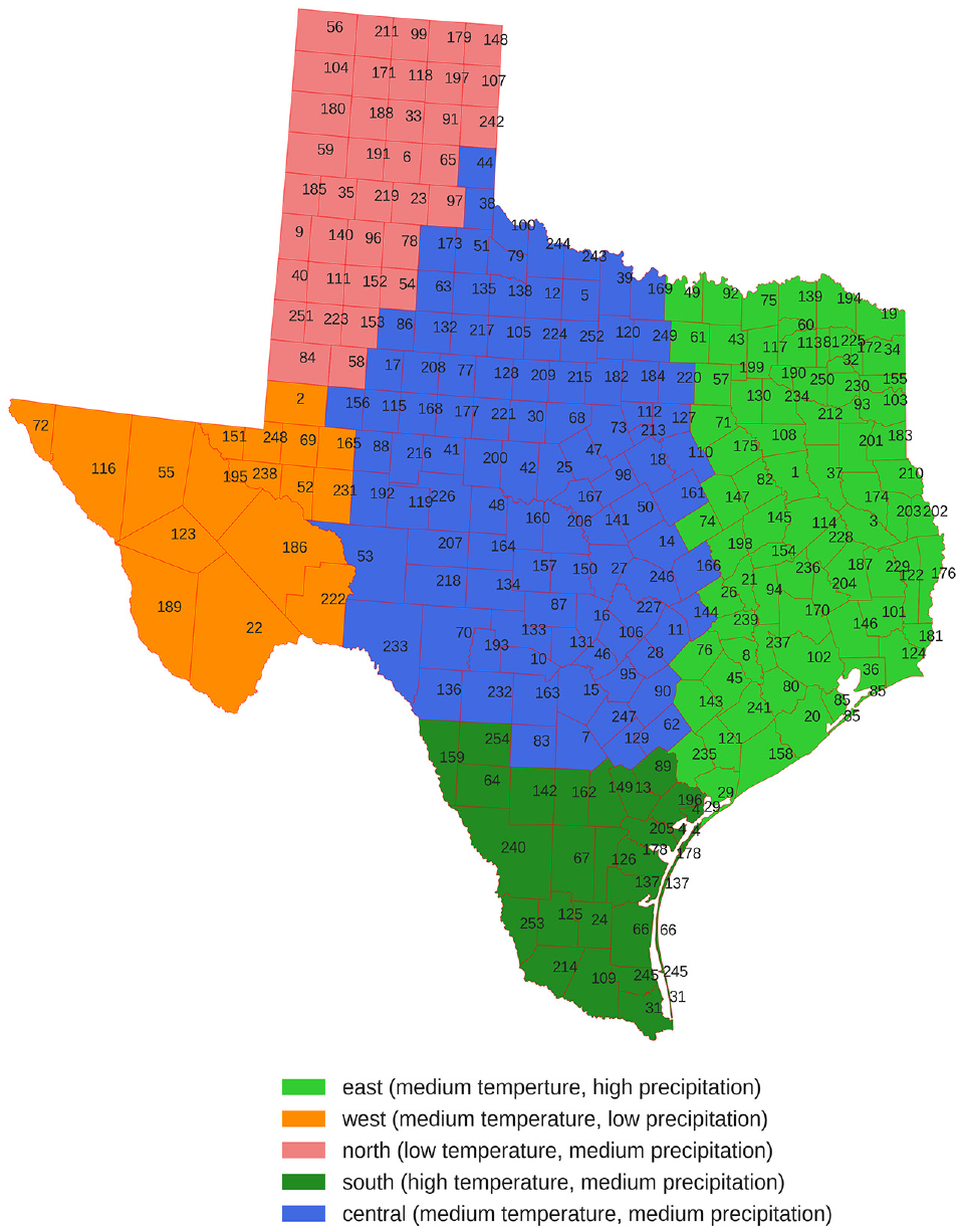
Climatic zones with county indexes.

Traffic

In this project, the 20-year projected equivalent single axle loads (ESALs) were used to represent the traffic characteristic of each pavement section. The distribution of the traffic is plotted in Figure 5.

Figure 5.

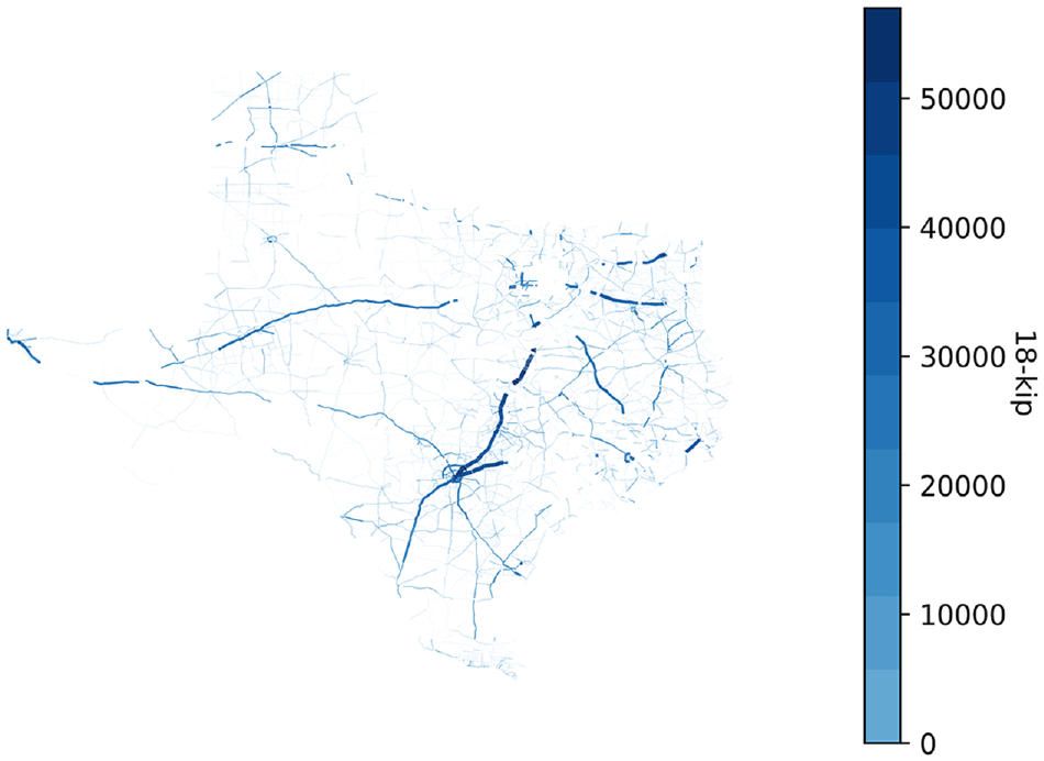
Map of traffic distribution.

Work History

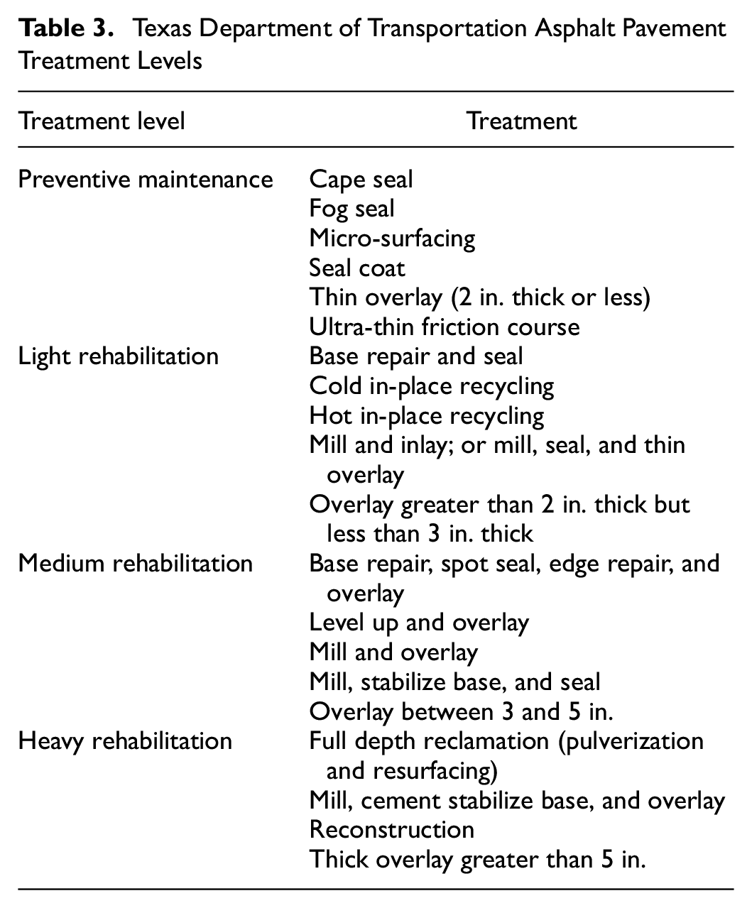
In this case study, we used pavement maintenance and rehabilitation history data collected by TxDOT. The maintenance dataset contains information about the type of treatments shown in Table 3, when they were implemented, and which pavement sections they were applied to. The work history records were converted to dummy variables representing each individual treatment when used in the modeling process.

Table 3.

Texas Department of Transportation Asphalt Pavement Treatment Levels

Treatment level	Treatment
Preventive maintenance	Cape seal
	Fog seal
	Micro-surfacing
	Seal coat
	Thin overlay (2 in. thick or less)
	Ultra-thin friction course
Light rehabilitation	Base repair and seal
	Cold in-place recycling
	Hot in-place recycling
	Mill and inlay; or mill, seal, and thin overlay
	Overlay greater than 2 in. thick but less than 3 in. thick
Medium rehabilitation	Base repair, spot seal, edge repair, and overlay
	Level up and overlay
	Mill and overlay
	Mill, stabilize base, and seal
	Overlay between 3 and 5 in.
Heavy rehabilitation	Full depth reclamation (pulverization and resurfacing)
	Mill, cement stabilize base, and overlay
	Reconstruction
	Thick overlay greater than 5 in.

Models

In this case study, we developed performance models for each of the 12 condition indicators using the standard machine learning models: the classification and regression tree (CART), NN, LR, and proposed GraphSAGE model. All machine learning models were implemented in scikit-learn ( 18 ) and default hyperparameter values were used. GraphSAGE models were implemented in PyTorch Geometric (PyG), which is a Python library supporting many types of deep learning on graphs. PyG makes it easy to build a deep learning model through customizing predefined GNN layers ( 19 ). We tuned the hyperparameters, number of layers, and number of hidden channels per layer by optimizing the model performance. We varied one hyperparameter at a time in this tuning process. For the GraphSAGE model, we finally chose two layers ( $K$ = 2), and the number of hidden channels of both layers was set to 256.

For each condition indicator’s deterioration model, the target variable is in its 2018 values and the features include 2014–2017 historical data of all condition indicators, maintenance work record, traffic, road functional class, climate zones, and pavement type information. We handle the interdependencies between condition indicators through including them in the others’ features. For example, when modeling the IRI as the target, previous years’ cracking, rutting, and patching ratings were used as features. The selection of the features is based on data availability and the pavement deterioration models currently used by TxDOT ( 17 ). Historical condition data from 2001 to 2017 were evaluated and the results show that the effect of historical conditions reach its maximum around 4–5 years. Data beyond that time range has little impact on model performance. As a result, the previous four years’ condition data (2014–2017) were included in the feature set. Some 20% of the dataset is used for testing and the rest for training the models. The R²-score, mean squared error (MSE), and mean absolute error (MAE) are used to measure and evaluate the performance of different models.

Results

The modeling results are provided in Table 4, which lists the R²-score, MSE, and MAE for each condition indicator. A negative R²-score indicates that the data cannot explain the target variable and the models perform poorly at predicting the testing set. It is probably because the target variables have little variation in the dataset. For each of the condition indicators, there are more than 110,000 data points (pavement sections). The number of data points used for each indicator was slightly different because of data availability. The proposed GraphSAGE model, which combines features from neighboring nodes, achieves better performance than the machine learning regression models using the scikit-learn library. The multivariate LR model, on average, has the best performance among the machine learning models. The worst performance is observed for the decision tree model. The best performances with respect to R²-score observed are for the IRI (0.87) and RS (0.85), both of which are measurements of the pavement roughness, and the RS is a linear transformation of the IRI. The reason why roughness models have better results than other indicators is probably because the deterioration of roughness (i.e., changes between consecutive years) is more linear compared with other distress indicators. The R²-scores for other condition indicators are between 0.10 and 0.60. While the multivariate LR model gives the best results among all machine learning models, the improvement brought by the GraphSAGE model ranges from 0% to 20% in relation to R²-scores.

Table 4.

Results of Different Models

	LR			CART			NN			GraphSAGE
Indicators	R ²-score	MSE	MAE	R ²-score	MSE	MAE	R ²-score	MSE	MAE	R ²-score	MSE	MAE
Shallow rutting	0.59	70.73	5.33	0.28	125.28	6.79	0.40	104.50	7.11	0.64	62.99	4.90
Deep rutting	0.47	6.51	1.16	0.00	12.42	1.39	0.44	6.84	1.29	0.51	6.00	1.04
Patching	0.11	30.33	2.08	−0.29	44.30	1.89	−0.40	47.90	3.50	0.31	23.51	1.70
Failures	0.08	0.44	0.15	−1.10	1.02	0.15	−0.24	0.61	0.33	0.12	0.43	0.12
Block cracking	0.08	6.43	0.66	−0.58	6.43	0.55	−56.55	404.82	11.00	0.13	6.11	0.49
Alligator cracking	0.17	16.59	1.71	−0.37	27.68	1.74	−0.42	28.72	2.87	0.35	13.07	1.43
Longitudinal cracking	0.15	351.33	11.76	−0.18	489.46	12.27	0.26	328.94	11.37	0.30	287.10	10.25
Transverse cracking	0.16	0.41	0.30	−0.28	0.64	0.27	−0.46	0.73	0.49	0.22	0.39	0.27
IRI	0.84	296.03	10.56	0.70	553.03	14.76	0.85	276.10	10.25	0.87	262.59	9.93
Ride score	0.85	0.07	0.17	0.70	0.14	0.24	0.08	0.46	0.45	0.85	0.07	0.17
Distress score	0.35	114.09	6.91	−0.15	203.71	8.49	0.35	114.33	6.89	0.43	100.27	6.27
Condition score	0.42	133.03	7.43	−0.03	241.69	9.26	0.42	134.92	7.92	0.50	115.77	6.78

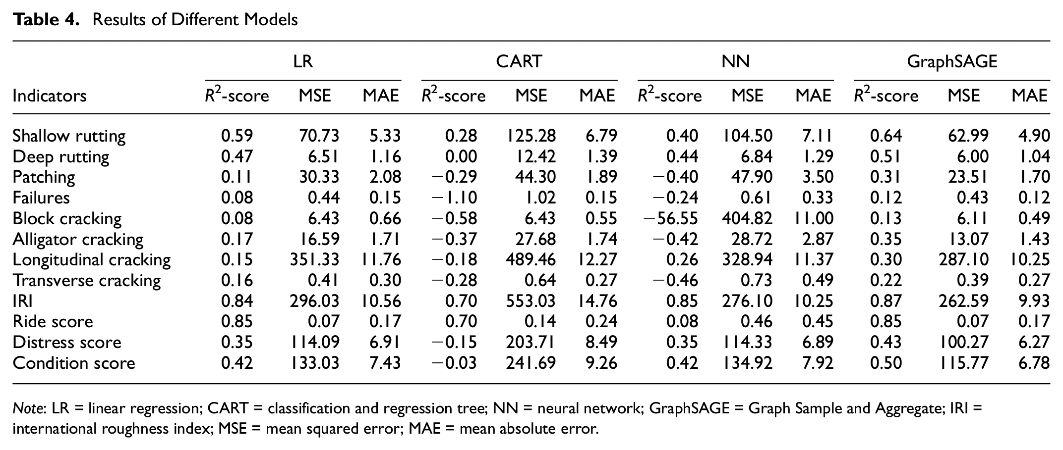
Note: LR = linear regression; CART = classification and regression tree; NN = neural network; GraphSAGE = Graph Sample and Aggregate; IRI = international roughness index; MSE = mean squared error; MAE = mean absolute error.

Figure 6 shows the training history of the GraphSAGE models. The modeling results are able to converge and achieve the highest R²-score after 100–800 epochs. The history for the training and testing dataset is labeled as training and the history for the testing dataset is labeled as testing. From the plots we can see that the models for longitudinal cracking and the CS could probably achieve a higher value of R-score if a few more epochs were trained, as the trend for R²-score on these datasets is still rising for the last few epochs. It can be found that the models for the indicators mentioned above have not been significantly over-learned in the training dataset, showing comparable performance on both training and testing datasets.

Figure 6.

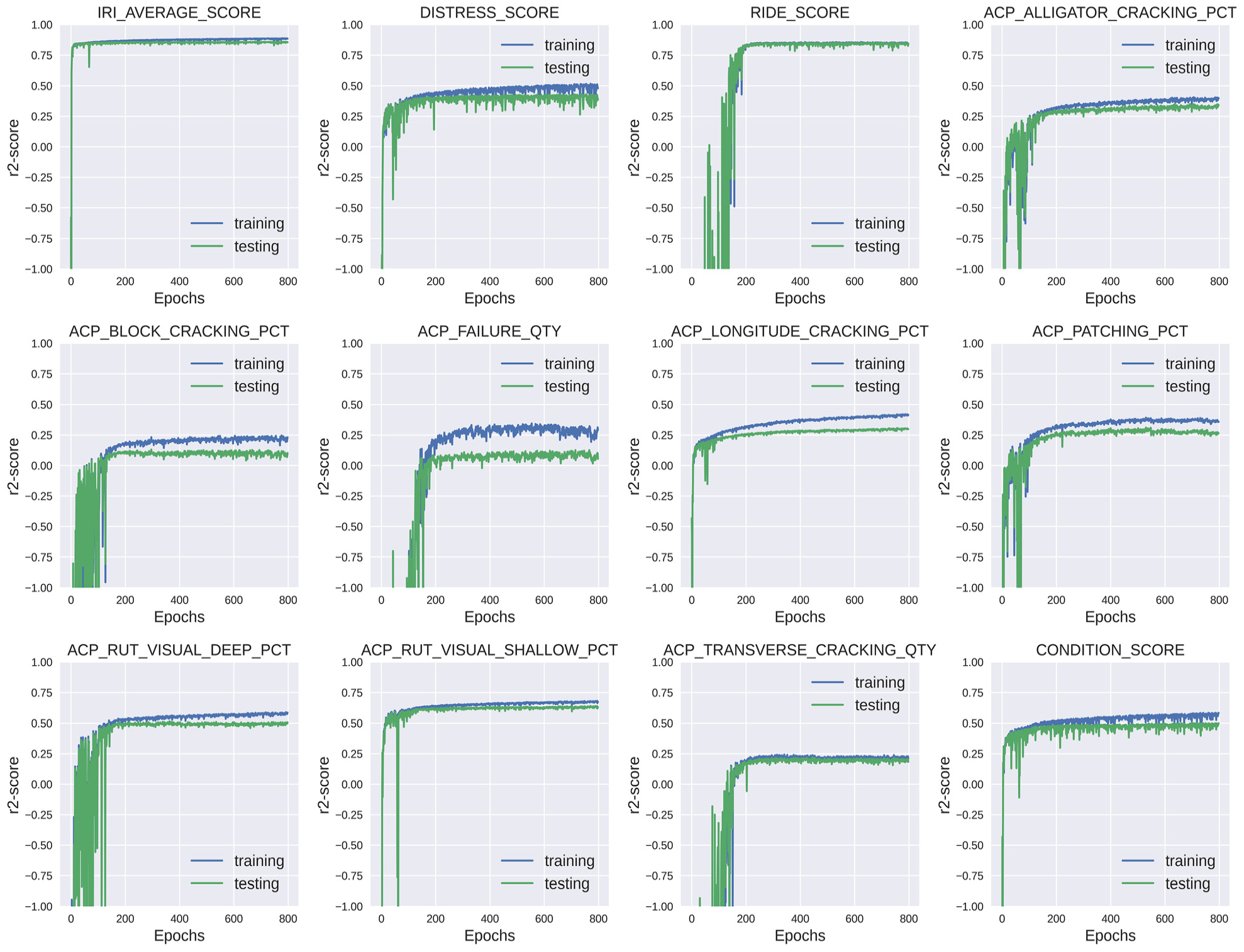
Training and testing R²-score versus epoch of the Graph Sample and Aggregate model.

Conclusions

In this paper, we used GNN models to analyze pavement condition data for performance prediction. The pavement network is considered as a graph combining historical condition inventory data and spatial connections between neighboring sections. The spatial relationship between a section and its neighboring sections were then taken into account when developing the deterioration models. The results show that our model outperforms other machine learning models on a large-scale real-world network with more than 100,000 nodes and edges. The best R²-score result, 0.87, was obtained for the IRI deterioration model. The developed model can assist engineers and administrators in more effectively managing pavement assets through improved deterioration prediction. The results of this research can be integrated into existing pavement management system through two approaches. One is to use the trained model directly for condition prediction and the other is to consider neighboring sections’ information when developing new deterioration models. The pavement sections used in this research were spatially coupled by using the unique reference marker stored in the TxDOT pavement management system. However, this approach can only recognize sections aligned linearly along the route. It does not recognize sections located nearby but not on the same route. Future research should include the latitude/longitude information of each section and consider sections within a certain radius. Future research can also address the interdependencies between condition indicators through combining all condition indicators into one multi-dimensional target.

Footnotes

Acknowledgements

The authors would like to thank all Texas Department of Transportation personnel who have helped this research study.

Author Contributions

The authors confirm contribution to the paper as follows: study conception and design: L. Gao, K. Yu; data collection: L. Gao; analysis and interpretation of results: L. Gao, P. Lu; draft manuscript preparation: L. Gao, K. Yu, P. Lu. All authors reviewed the results and approved the final version of the manuscript.

Declaration of Conflicting Interests

The author(s) declared no potential conflicts of interest with respect to the research, authorship, and/or publication of this article.

Funding

The author(s) disclosed receipt of the following financial support for the research, authorship, and/or publication of this article: This work was supported by the Texas Department of Transportation Grant 0-6988.

ORCID iDs

Lu Gao

Ke Yu

Pan Lu

All opinions, errors, omissions, and recommendations in this paper are the responsibility of the authors.

References

Zou

Madanat

Incorporating Delay Effects into Airport Runway Pavement Management Systems. Journal of Infrastructure Systems, Vol. 18, No. 3, 2012, pp. 183–193.

Atef

Moselhi

Modeling Spatial and Functional Interdependencies of Civil Infrastructure Networks. Proc., Pipelines: From Underground to the Forefront of Innovation and Sustainability, Portland OR, ASCE, Reston, VA, 2014, pp. 1558–1567.

Bernhardt

K. L. S.

McNeil

Center

U. T.

An Agent Based Approach to Modeling the Behavior of Civil Infrastructure Systems. Proc., Engineering Systems Symposium, Tang Center, MIT, 2004.

McDaniels

Chang

Peterson

Mikawoz

Reed

Empirical Framework for Characterizing Infrastructure Failure Interdependencies. Journal of Infrastructure Systems, Vol. 13, No. 3, 2007, pp. 175–184.

Rahman

H. A.

Beznosov

Martí

J. R.

Identification of Sources of Failures and their Propagation in Critical Infrastructures from 12 years of Public Failure Reports. International Journal of Critical Infrastructures, Vol. 5, No. 3, 2009, pp. 220–244.

Panzieri

Setola

Ulivi

An Agent based Simulator for Critical Interdependent Infrastructures. Proc., Securing Critical Infrastructures, CRIS2004: Conference on Critical Infrastructures, France, Grenoble, 2004, pp. 25–27.

Lee

Sun

Lee

Development of Deep Learning based Deterioration Prediction Model for the Maintenance Planning of Highway Pavement. Korean Journal of Construction Engineering and Management, Vol. 20, No. 6, 2019, pp. 34–43.

Choi

Development of the Road Pavement Deterioration Model Based on the Deep Learning Method. Electronics, Vol. 9, No. 1, 2019, p. 3.

Hosseini

S. A.

Alhasan

Smadi

Use of Deep Learning to Study Modeling Deterioration of Pavements a Case Study in Iowa. Infrastructures, Vol. 5, No. 11, 2020, p. 95.

10.

Gao

Hao Ren

Detection of Pavement Maintenance Treatments Using Deep-Learning Network. Transportation Research Record: Journal of the Transportation Research Board, 2021. 2675: 1434–1443.

11.

Haddad

A. J.

Chehab

G. R.

Saad

G. A.

The Use of Deep Neural Networks for Developing Generic Pavement Rutting Predictive Models. International Journal of Pavement Engineering, Vol. 23, No. 12, 2021, pp. 4260–4276.

12.

Zhou

Okte

Al-Qadi

I. L.

Predicting Pavement Roughness Using Deep Learning Algorithms. Transportation Research Record: Journal of the Transportation Research Board, 2021. 2675: 1062–1072.

13.

Gao

Missing Pavement Performance Data Imputation Using Graph Neural Networks. Transportation Research Record: Journal of the Transportation Research Board, 2022. 2676: 409–419.

14.

Zhou

Cui

Zhang

Yang

Liu

Wang

Sun

“Graph Neural Networks: A Review of Methods and applications.”

AI Open, Vol. 1, 2020, pp. 57–81.

15.

Hamilton

Ying

Leskovec

Inductive Representation Learning on Large Graphs. Advances in Neural Information Processing Systems, Vol. 30, 2017, pp. 1025–1035.

16.

TxDOT. “Highway Designations Glossary.”Texas Department of Transportation. https://www.txdot.gov/inside-txdot/division/transportation-planning/highway-designation/glossary.html. Accessed July 5, 2022.

17.

Kim

M. Y.

Sabillon

Gao

Prozzi

J. A.

Development of Pavement Performance Models for Pavement Management Incorporating Treatment Type. Report No. FHWA/TX-21/0-6988-2. University of Texas at Austin, Center for Transportation Research, 2021.

18.

Buitinck

Louppe

Blondel

Pedregosa

Mueller

Grisel

Niculae

, et al. “API Design for Machine Learning Software: Experiences from the Scikit-Learn Project.” arXiv preprint arXiv:1309.0238, 2013.

19.

Matthias

Lenssen

J. E.

Fast Graph Representation Learning with PyTorch Geometric. Proc., ICLR Workshop on Representation Learning on Graphs and Manifolds, New Orleans, LA, 2019.