
Abstract
Road crashes are a prevalent public health issue across the globe. The objective of this research was to develop a methodology for accurately classifying high-risk crash locations. The hypothesis of this study was that readily obtained roadway indicators can be used along with machine learning techniques to categorize locations as high crash-risk. A database containing 5,383 locations was created during 2012 to 2015 as part of the Hellenic National Road Safety Project and used to develop three binary machine learning models to classify high crash-risk locations based on roadway indicators. The three models were random forest, gradient boosting, and extra trees. This research used features engineering to reduce the number of indicators in the model, and the synthetic minority oversampling technique to address imbalances in the dataset between the minority (high crash-risk locations identified using crash reports) and majority classes (medium to low crash-risk locations identified based on local police testimonies, site inspections, and geometry analysis). Although all three models performed similarly, the extra trees model outperformed the other two on a range of performance metrics, including the area under the precision–recall curve and the F1-score. The findings revealed that design speeds, pavement markings, signage presence, and pavement condition were the most influential factors affecting roadway safety. The contribution of this research is in the development of a transferable methodology for classifying high crash-risk locations in addition to revealing key indicators for crash-risk potential, which in turn can inform cost-effective data collection and maintenance activities.
Keywords
Crashes are prevalent on roadway networks worldwide, contributing to a global public health crisis. Every year approximately 1.35 million people lose their lives in roadway crashes ( 1 ) and an estimated 20 million to 50 million are affected by severe injuries owing to their involvement in a crash ( 2 ). Research has shown that crashes are correlated with certain location characteristics (i.e., geometric and surface roadway conditions and weather) ( 3 ), as well as driver behavioral factors ( 4 – 6 ). Although behavioral factors can be determined and addressed via training and enforcement, road crashes cannot be eliminated without the proper design and maintenance of roadways and their environment. Thus, the need to understand the key crash-contributing roadway factors to update design guidelines and inform the implementation of countermeasures and maintenance activities to prevent crashes is critical.
Typical statistical methods, such as logistic regression ( 7 , 8 ), negative binomial models ( 9 , 10 ), ordered probit models ( 9 , 11 ), and Bayesian network models ( 12 , 13 ) have been widely used in crash injury severity analysis. However, such models are limited by the assumptions of the relationship between dependent and independent variables. An additional limitation is that some of these traditional approaches cannot model discrete variables. Machine learning (ML) techniques have been demonstrated to overcome some of the limitations associated with traditional statistical models ( 14 , 15 ). The potential benefits of ML methods are (i) their ability to manage high-dimensional problems, (ii) their flexibility with complex data structures, and (iii) their predictive potential via the extraction of rules ( 16 ). Barai presents a variety of ML applications in transportation engineering, including roughness analysis, pavement analysis, and road crash analysis ( 17 ).
The objective of this research was to develop transferable ML models for classifying high crash-risk locations using data from the Hellenic National Road Safety Project. This project was funded by the Greek Ministry of Infrastructure and Transportation during 2012 to 2015, with the goal of identifying high crash-risk locations within the national and regional road network of the country. The primary interest was to identify which roadway environmental factors have a significant negative impact, thus influencing the probability of crash occurrence, and to inform implementation of remedial measures based on cost–benefit criteria. Data from a total of 15,000 km (9,300 mi) and 7,000 locations were recorded, creating a database of 35 road indicators related to a locations’ geometric design, pavement markings, and signage.
Machine Learning for Crash Frequency and Severity Prediction
Several studies have used ML methods to understand the factors affecting crash frequency and severity and to develop models for crash prediction. ML methods that have been applied vary between rule-based methods, such as association rule making, which attempt to understand how the combination of certain factors affect crash outcomes ( 3 ), and others such as support vector machine (SVM) (15, 18–20), the K-means algorithm ( 3 , 21 ), and neural networks ( 4 , 13 , 19 , 22 , 23 ), which can be used for crash location classification (e.g., based on crash frequency or severity) and therefore crash or injury and severity occurrence prediction. Other studies include decision tree techniques ( 19 , 21 , 22 , 24 ), and naive Bayes ( 21 ). The majority of these methods have focused on predicting crash severity once a crash has been identified.
Several factors have been considered in these studies, such as road geometric and environmental factors, weather, pavement conditions, traffic conditions, and driving behavior. More specifically, crash outcomes (i.e., crash severity) have been correlated with alcohol/drugs, seat belt use, and other driver behavioral factors (e.g., speeding) ( 4 – 6 ), demographic characteristics such as age and gender ( 4 , 22 ), roadway geometry (e.g., curve length, shoulder width) ( 8 , 15 , 22 ), absence of median barriers ( 13 ), roadway conditions (e.g., wet road surfaces, lighting conditions) ( 8 , 22 , 23 ), traffic conditions ( 13 ), speed limits ( 8 ), and crash type (e.g., between vehicles and nonmotorized users, roll over crashes) ( 25 ).
Multiple ML techniques, including SVM, fuzzy C-means-based SVM, feed-forward neural networks (FNN) and fuzzy C-means clustering-based FNN, were implemented by Assi et al. to classify locations by crash injury severity (severe and nonsevere crashes) and determine the most influential factors among human, vehicle, roadway, and environmental characteristics ( 18 ). However, the basis for selecting the most important factors was to utilize the most easily available data from crash sites and no effort was made to reduce the number of contributing factors.
Overall, existing literature has showcased the advantages of using ML methods for crash frequency and crash severity prediction. However, few studies have focused on predicting crash frequency, that is, classifying locations as high-risk based on crash frequency. Most importantly, crash frequency and -severity prediction models often lack the capacity to extract the most important features contributing to crashes or crash severity ( 19 ) because they rely on the most easily available data from crash sites ( 18 ). Those that have made such attempts have investigated correlations between variables to eliminate certain indicators ( 20 , 26 ), conducted sensitivity analyses to assess the impact of various factors on crash severity ( 15 , 25 ), or used variable importance measures ( 5 ). This is important, as it can significantly reduce the need for data collection, therefore, requiring fewer resources that can facilitate cost-effective maintenance and safety improvement activities. To our knowledge, no other study has used feature engineering to extract the most influential factors in addition to threshold analysis to identify model parameters and underlying functions that could improve model performance.
Contributions
This research contributes to the existing body of literature in multiple ways. First, it uses feature engineering to determine the most relevant road characteristics contributing to crashes. This is a critical step when working with large datasets from both a methodological and application standpoint. Methodologically, a reduction in the number of features to be considered results in better performance models ( 27 ). Practically, fewer parameters allow for faster training with a reduced number of roadway indicators, therefore facilitating transferability. In addition, identifying the most critical factors through feature engineering contributes to the cost-effectiveness of maintenance activities and other safety countermeasures.
Second, this research illustrates the use of ML methods for imbalanced datasets, as previous studies focusing on correlations between roadway characteristic and crashes, have assumed balanced dataset distributions. Further, this is the first study to correlate location characteristics with crashes by applying techniques for imbalanced datasets.
Finally, this study performs threshold analysis when utilizing ML techniques. Because of the imbalanced nature of the problem, the default threshold is not the best way to understand the anticipated probability of the minority class, since the threshold governs the choice to turn a projected probability into a class of engineering purpose. In this study, threshold analysis was used to optimize the prediction of high-risk crash locations, by finding a balance between the correctness and the proportion of high crash-risk location predictions.
The rest of the paper is organized as follows. First, a summary of the literature related to the use of ML models for understanding crash-contributing factors and predicting crash frequency and severity is presented. Next, the dataset used is described, followed by a summary of the feature engineering approach. The following section describes the remainder of the methodology by addressing the imbalanced dataset issue and continuing with the development of the three binary ML models, namely, random forest, gradient boosting, and extra trees, and a description of the performance measures used. In the results section, we compare the performance of the three models, conduct a threshold analysis, and present the ranking of the most important roadway features for crash prediction. Finally, the conclusions section summarizes the main methodological contributions and findings, discusses limitations, and outlines directions for future research.
Data
Hellenic National Road Safety Project
Greece has the sixth highest rate of crash fatalities among the 27 members of the European Union based on 2019 data ( 28 ), which can be partially attributed to the lack of an effective study of road crashes ( 29 ). To improve road safety and reduce the number and severity of road crashes, the Greek Ministry of Infrastructure and Transportation in collaboration with the public agency Egnatia Odos S.A. started developing a Road Infrastructure Safety Improvement program implementing EU Directive 2008/96/EC ( 30 ). A main goal of the project, which spanned the years 2012 to 2015, was to identify high crash-risk locations within the 15,000-km (9,300-mi) road network and apply remedial measures based on cost–benefit criteria. This network consists of 4,200 km (2,600 mi) of national roads and 10,800 km (6,700 mi) of regional roads.
The primary interest of the project was to determine which roadway environmental factors are critical in predicting the probability of a crash. Contributing factors related to human, vehicle, traffic, or weather conditions were not included in the analysis. Nevertheless, the identification of geographic locations alone can still inform inventory and maintenance activities. In addition to inventorying high/medium crash-risk locations, the project was also intended to promote remedial measures based on cost–benefit criteria.
The implementation of the project was based on identification of locations where crashes have occurred or identification of locations with low safety standards according to site inspection and geometric characteristics. Three main categories of roadway classification safety were taken into consideration to group crash-risk locations, namely, proven, testimony, and potential.
Proven: locations where crashes have occurred based on police crash reports codified into the National Road Accident Database by the Hellenic Statistical Authority. These locations were classified as high crash-risk locations.
Testimony: locations with crash data based on site inspections data or testimonies (no official reports) from local police stations and road maintenance authorities, collected via surveys. These locations were classified as medium crash-risk locations.
Potential: locations where crashes are yet to occur (or have happened but were never recorded) but may do so in the future. Crash-risk was based on their geometric characteristics, identified by inspection and assessment of road data, GPS measurements, video recording, onsite inspections, and geometric analysis. These locations were classified as low crash-risk locations.
Through analysis of the collected information, 7,000 locations were inventoried and classified as above (see Figure 1). Each location in the database was described by 35 roadway indicators (as shown in Table 1), which can be considered as having a potential negative impact on crash occurrence. Selection of the appropriate roadway indicators followed the National Road Works Design Guidelines ( 31 ), representing roadway environmental factors in eight main categories: inspection, safety, road geometry, road surface, drainage, interchanges, speed, and location length. The value for each indicator represents the length, which is the detection length of the road indicator.
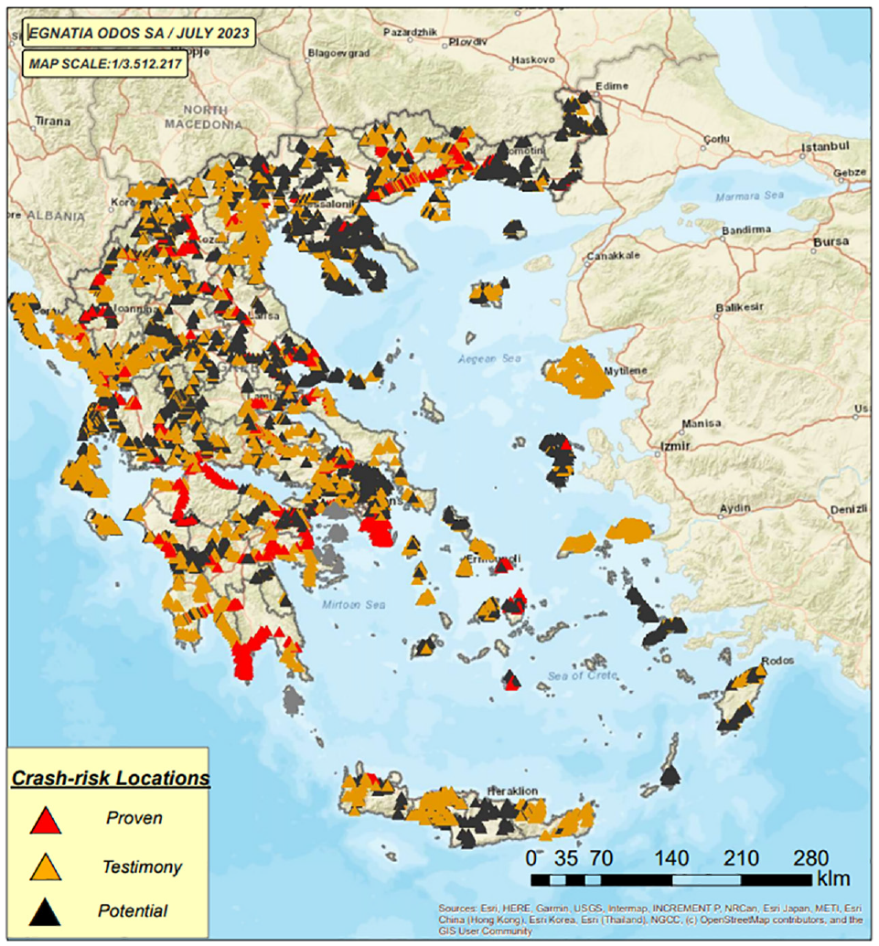
Locations of crash risk across 15,000 km (9,300 mi) of road network in Greece.
Indicators as Features

Note: L = left side; R = right side (representing detection length).
The project used this database for road safety assessments that included cost–benefit procedures and crash reduction factor analysis ( 32 ), which resulted in remedial measures implementation of both short-term (e.g., repairing pavement, road markings, safety barriers) and medium-term measures (e.g., provision of a by-pass, roundabouts).
Dataset
A dataset of 5,383 locations, out of a total of 7,000, was collated from the Hellenic National Road Safety Project for use in this study. The 35 roadway indicators with negative safety impacts were used as the predictor variables, whereas the roadway safety classifications—proven, testimony, and potential—were the target variables for the model development. Table 1 shows the corresponding dataset of features. Indicators 1 to 30 were recorded separately for the left and right sides of the roadway, resulting in a total of 60 features. Indicators 31 and 32 included records for both sides of the roadway, thus yielding a total of two features. Indicators 33 and 34 represent segment lengths classified as “not acceptable” (33n and 34n) and “acceptable” (33a and 34a). Indicator 35 consists of only one feature, which is the length of the roadway location’s segment. Overall, there were 67 length detection features. In the dataset, zero-valued observations (in features corresponding to Roadway Indicators 1 through 34) did not indicate missing values. Instead, they indicated that the detection length of the segments for those observations was zero, and thus, the negative impact of the feature was absent for the given segment.
In this study, the three roadway classification safety categories were grouped into two. Proven locations were categorized as “crash characteristics” (CCs), whereas both testimony and potential locations were grouped into the “possible crash characteristics” (PCCs) class. Proven locations were identified as high crash-risk using a crash analysis approach based on formally reported crashes. On the other hand, testimony and potential were locations where crash-risk was medium to low since this classification was based on site inspection data, testimonies, and geometrical characteristics and typically included low severity or property damage only crashes. The final dataset contained 351 locations characterized as proven, 2,401 locations as testimony, and 2,631 locations characterized as potential. Grouping these into two classes as described resulted in 351 locations being labeled as CCs and 5,032 as PCCs.
Methodology
The research methodology involved the following three aspects: feature engineering, feature selection, and model development. Three machine learning (ML) models—random forests, extra trees, and gradient boosting machine—were trained using the dataset described in the previous section. These models employed an ensemble learning approach using decision trees as the base models. In random forests ( 33 ), each decision tree is fitted by randomly selecting a feature from a fixed-size subset that is used to optimize the predictive performance of the tree at each branching step. Furthermore, bootstrap samples are used to populate the ensemble. The extra trees model differs from random forests in that the splitting feature is randomly chosen from the entire set of features at each node and the ensemble is created by running the same algorithm on the original training sample ( 34 ). The gradient boosting machine can be considered an additive model of weak learners (in this case, shallow decision trees) in which each successive base learner corresponds to a gradient update in estimating the fitted machine ( 35 ).
The objective of training these models was to classify locations as CCs or PCCs based on the 35 roadway indicators and to ultimately facilitate a better understanding of the relationship between roadway indicators and crash risk (inference) as well to identify a new CC locations based on the selected features.
Feature Engineering
Feature engineering is used to extract features into suitable formats for the application of an ML model. This is a very important step in the ML pipeline, because with suitable features a model can be improved and produce a higher quality output ( 8 ). All 67 features in the dataset were numerical variables representing length.
Removing Quasi-Constant and Duplicated Features
Typically, features are characterized as quasi-constant when 99% of the observations contain the same value for this feature, but this could vary somewhere between 95% to 99%, depending on the dataset. In general, these features provide little, if any, information that allows an ML model to discriminate or predict a target ( 36 , 37 ).
Identifying and removing quasi-constant features is an easy first step toward feature selection and more interpretable ML models. Exploring the dataset using 99% threshold, resulted in 11 of the initial 67 features being quasi-constant, leaving 56 features for further model development.
When two features in the dataset show the same value for all the observations, they are in essence the same feature, and thus, one can be removed. A search through the dataset identified Indicators 6, 7, and 28 as having duplicate features, that is, the same values were reported for each of those indicators for the left- and right-side features. Thus, we removed three duplicate features from the set of 56, leaving a total of 53.
Correlated Features
If two predictor variables are highly correlated, they provide redundant information about the target, as just one of them is sufficient for prediction. The feature engineering method of identifying groups of correlated features was used to determine 13 correlated features: 1L, 3L, 4R, 5R, 9L, 14R, 19L, 21R, 22L, 24L, 29L, 34a, and 35. Removing these highly correlated features, we were left with 40 features in the dataset.
Feature Selection
The main objective of feature selection in supervised learning is to identify the subset of features that produces the best classification performance. This allows for improved learning efficiency and predictive accuracy, while reducing the complexity of learned results. Random forest decision tree models were independently fitted for each of the 40 features to predict each location’s class. Thus, 40 models were estimated. The area under the receiver operating characteristic (ROC) curve (AUC) was then used as the performance metric ( 38 , 39 ). The ROC curve plots the true positive rate against the false positive rate for various thresholds and the AUC is a global measurement of the model performance across the various thresholds. Maximum performance corresponds to an AUC value of 1. However, an AUC value of 0.5 indicates a random decision and thus serves as the baseline threshold for classifier performance. Thus, if a model trained on one feature has an AUC greater than 0.5, then the feature has some explanatory power. Figure 2 shows the AUC for the univariate decision tree classifiers fitted on each corresponding feature. In this case, 26 features exhibited AUC values greater than 0.5 (threshold depicted by dashed red lines), and were therefore selected for inclusion in the final dataset.

Area under the receiver operating characteristic curve (AUC) of the 40 univariate random forest models each fitted with its corresponding candidate feature. The AUC > 0.5 selection threshold is indicated by red dashed lines.
Before proceeding with the training of the three models, we pursued a performance comparison with the initial dataset including 67 features versus the updated dataset containing 26 features. Both datasets were split into training and test datasets (using a 70:30 split). Several performance metrics were used to compare model results based on both datasets, as shown in Table 2. Accuracy was defined as follows:

where
Machine Learning Performance Between Initial (i.e., 67 Features) and Final (26 Features) Dataset

Note: AUC = area under the receiver operating characteristic curve.
Recall was defined as the proportion of actual positives that were identified correctly, whereas precision was the proportion of positive identifications that were actually correct ( 40 , 41 ) and were calculated based on the following equations:


Finally, the F1 score is a weighted harmonic mean of the precision of the record and varies between 0 and 1, 1 being the ideal value ( 41 ). This metric offers the best balance between precision and recall, which is achieved by the selection of an appropriate threshold that maximizes it. This is given by

The results indicated that using either the 67 initial features or the 26 filtered ones to train the models to predict crash risk resulted in similar performance in relation to accuracy, recall, and AUC. However, the models trained using the filtered dataset performed better with regard to precision and F1 score. This highlights the potential cost-saving impact of feature selection, since only 40% of the initial set of 67 indicators were needed to predict crash risk.
Model Training and Development
Data Splitting
As before, 70% (3,768 observations) of the initial dataset of 5,383 observations were used for the training of all three models, and the remaining 30% (1,615 observations) were reserved for testing. The distribution of observations across the classes in each set is shown in Table 3.
Number of Samples in Training and Test Sets

Note: PCCs = possible crash characteristics; CCs = crash characteristics.
Oversampling of Minority Class
Imbalanced datasets are those that have many more instances or observations of a certain class compared with other classes. Many real-world data mining applications involve datasets from strongly imbalanced distributions concerning the target variable ( 42 ). In recent years, the imbalanced learning problem has drawn a significant amount of interest from academia, industry, and government funding agencies. The majority of standard algorithms assume or expect balanced distributions concerning the class or equal misclassification costs ( 43 ). Therefore, in highly imbalanced datasets, algorithms fail to properly represent the actual data distributions, leading to inaccurate predictions. This renders accuracy an inappropriate performance measure for imbalanced datasets, as it does not provide an estimation of how the model is performing in each of the classes. For a binary problem, the degree of imbalance of a class distribution can be denoted by the ratio of the sample size of the minority class to that of the majority class, as shown in Equation 5 ( 44 ),

where X(minority) is the number of observations in the minority class and X(majority) is the number of observations in the majority class. In some cases, a ratio as low as 1:35 can be hard to classify, whereas in other cases even a ratio of 1:10 can be problematic. In this study, the imbalanced ratio was 1:14.3, which showed a strongly imbalanced dataset with CCs as the minority class and PCCs as the majority class. To address this, an oversampling (data augmentation) method for the minority class, referred to as the synthetic minority oversampling technique (SMOTE) was applied (Figure 3) ( 45 – 50 ). This approach involves creating new observations in the minority class by interpolation, thus avoiding duplication. After applying SMOTE, the number of CC observations in the training set increased from 249 to 3,519, allowed for an equal number of samples in both classes.
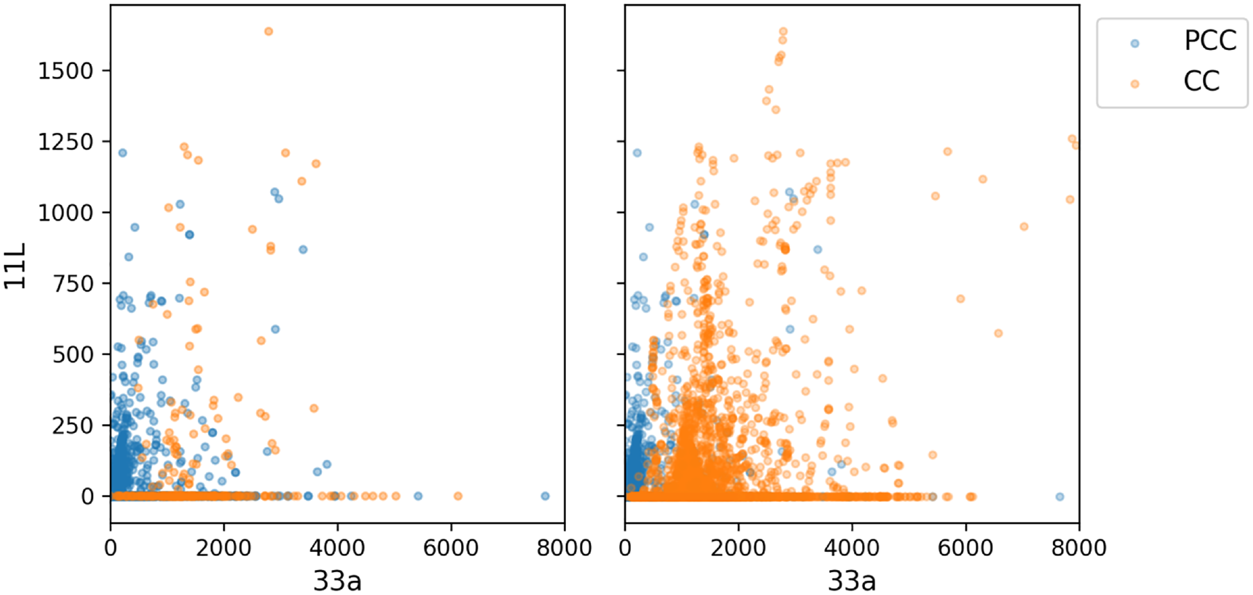
Example of scatter plots showing values of two features, Cases 11L versus 33a: (a) original (imbalanced) training set, and (b) SMOTE-augmented (balanced) training set.
Model Development
Three ML models for supervised learning were fitted in the study: random forest ( 33 ), gradient boosting machine ( 35 ), and extra trees ( 34 ). The ML models were developed on the train SMOTE-augmented dataset following a systematic procedure of parameter tuning via grid search. The test dataset was used to assess the model performance using similar performance measures as described earlier: precision, recall, accuracy, and F1 score.
Results
Performance Metrics
Table 4 shows the performance of the three models, as well as the optimal parameters found via grid search (number of estimators and maximum tree depth). Although the accuracy score of 0.95 reported for these models seems impressive it did not distinguish between the numbers of correctly classified observations of the different classes. In fact, the minority class (in our case CCs) had very little impact on the overall accuracy value compared with the majority one. Thus, we considered the other performance metrics. As seen in Table 4, the extra trees classifier had the highest recall and F1 scores of 0.76 and 0.66, respectively.
Model Performance

Note: na = not applicable.
Receiver Operating Characteristics and Precision–Recall Curves
To further investigate the performance of the models across all possible classification thresholds, we plotted the receiver operating characteristics (ROC) curve and precision–recall curve (PRC). The corresponding metrics of interest were the area under the ROC curve (AUC) and the area under the PRC (AP). Figure 4 shows the ROC curves and corresponding AUC values for all three models, while Figure 5 shows the PRC and corresponding AP values for the models. The extra trees models still demonstrated the best performance among the three models, with an AUC of 0.95 and an AP of 0.71. These results further confirmed that the extra trees classifier was the best performing model for this dataset.
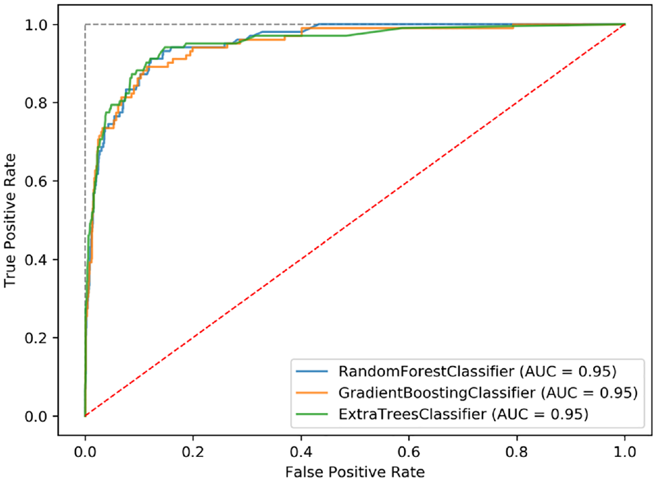
Receiver operating characteristic curves and AUC values for the three models.
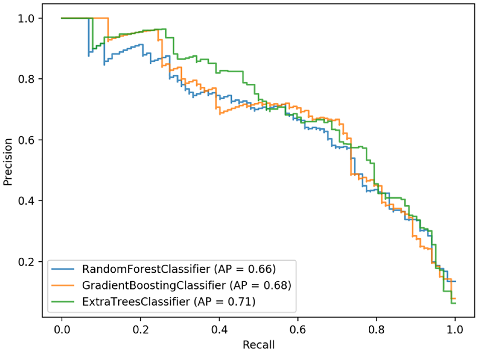
Precision–recall curves and AP values for the three models.
Threshold Analysis
The decision for converting a predicted probability into a class label is governed by a parameter referred to as the threshold (θ). The default value for a threshold is 0.5 for normalized predicted probabilities or scores in the range between 0 and 1. However, for classification problems that have a class imbalance, the default threshold can result in poor performance. The probability threshold for assignment to a positive class can be selected to optimize the performance measure of interest—this was critical in our case, the positive class being the CCs.
In Figure 6, we show the performance metrics generated for various threshold values from 0 to 1 for the extra trees model. The best performance for predicting the CC class, with reference to Equation 2, was when the recall value was high. By selecting a high recall value we made a rule for predicting most true cases from the CC class, but at the same time we generated many false CC predictions, since precision was low (Equation 3). As a result, the recall value expressed the percentage of detecting the true cases in the CC class, whereas precision detected the percentage of correct CC predictions in the predictive sample. Therefore, the optimum performance rule for predicting the CC class for practical use requires a cost-sensitive analysis and engineering judgment.
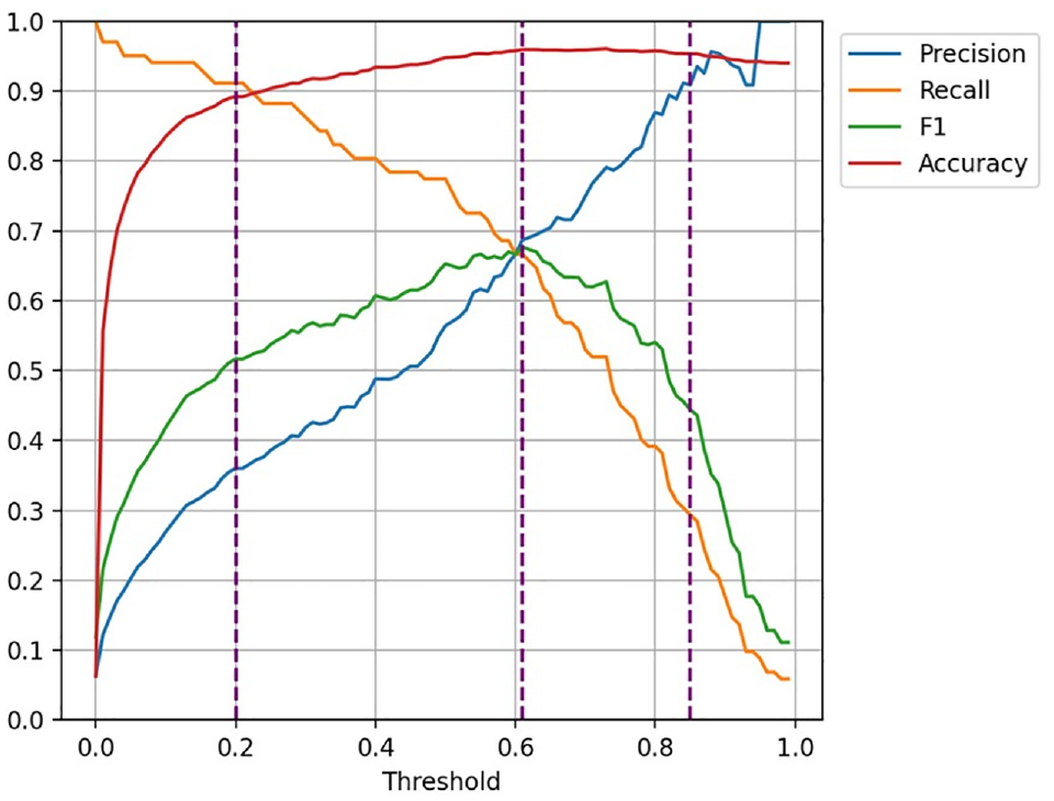
Precision, recall, F1 score, and accuracy values at thresholds from 0 through 1 for the extra trees model. Selected thresholds for analysis (0.2, 0.61, and 0.85) are depicted with purple dashed lines.
In our case, we considered three scenarios of threshold values, θ, at 0.20, 0.61, and 0.85 to give an idea of the importance of the value, θ, for predicting the CC class. The θ = 0.2 scenario tended toward recall optimization, whereas the θ = 0.85 scenario tended toward precision optimization. However, θ = 0.61 was the optimal point for the F1 score (which was also where both recall and precision were maximized). The corresponding confusion matrices for these thresholds, indicating the true negatives, FPs, false negatives, and true positives (TPs), are shown in Figure 7. The performance metrics for each threshold scenario are summarized in Table 5.
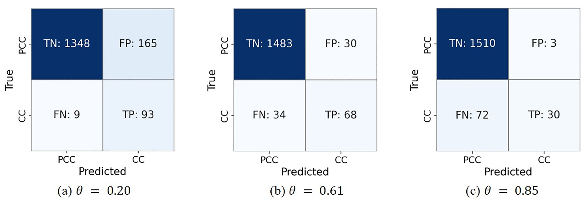
Confusion matrices for the extra trees classifier at various probability thresholds, θ.
Model Performance

The test dataset included 102 true cases of CCs and 1,513 true cases of the PCC class. On the one hand, a probability threshold of θ = 0.20 resulted in a recall score of 0.91 and a precision score of 0.36. In this high-recall scenario, the model predicted the majority (91%) of CC samples but only 36% of CC predictions were correct; that means that 64% of CC (positive) predictions were misclassified. According to the confusion matrix (Figure 7a), there were 165 samples misclassified as CCs, that is, FPs. From an engineering aspect, although the model detected the majority of CC locations, 64% of the predictive samples will be misclassified as CC locations, which may lead to unnecessary safety measures, and thus higher mitigation costs, since CCs are classified as high crash-risk locations.
On the other hand, assuming a probability threshold, θ = 0.85, yielded a recall score of 0.29 and a precision score of 0.91, in this high-precision scenario, only 29% of CC locations would be predicted correctly, however, only 10% of the predictive samples were misclassified as CC predictions. Thus, from the engineering perspective, this scenario represents a conservative approach that prioritizes the correctness of CC predictions. Consequently, less money is needlessly spent on safety measures, as there are few (10%) misclassified CC predictions; yet, the safety risk was much greater than in the θ = 0.2 case, as 71% of CC high crash-risk cases went undetected (Figure 7c).
Finally, we considered a scenario that optimized for the F1 score at the maximum value of 0.68. This occurred at a probability threshold of θ = 0.61. Here, recall was 0.67 and precision was 0.69. Thus, 67% of CC locations were predicted correctly and 33% were misclassified. This threshold represented the optimal balance between precision and recall, as neither score could be further improved without diminishing the other. For the decision maker, this suggests the best tradeoff between unnecessary spending on safety measures and the reduction in crash risk resulting from correct predictions.
Feature Importance
We ranked the features in the extra trees model based on the mean decrease in node impurity, which indicated how the choice of a certain feature in tree construction contributed to the accuracy of the tree’s prediction. Thus, the mean decrease in node impurity served as a measure of the importance or relevance of a given feature to the target variable. We show the feature importance values for the selected extra trees model in Figure 8. (We refer the reader to Table 1 for a complete summary of the roadway indicators and features.) Based on the ranking, the 10 most important features, along with their corresponding indicator descriptions, were:
Feature 33a: Unacceptable harmony between design speed and operating speed (Safety Criterion I) and in particular, the length classified as acceptable length;
Feature 6L: Incomplete lane marking;
Feature 8L: Incomplete pavements markings;
Feature 19R: Road surface cracks along the road (transverse meandering);
Feature 3R: Incorrect or incomplete danger signs;
Feature 4L: Incorrect or incomplete speed limits signs, and so forth;
Feature 22R: Alligator cracking;
Feature 10L: Incomplete safety issues;
Feature 11R: Incorrect terminals (parapets, ends of barriers); and
Feature 34n: unacceptable harmony and continuity of operating speed (Safety Criterion II) and in particular, the length classified as not acceptable length.
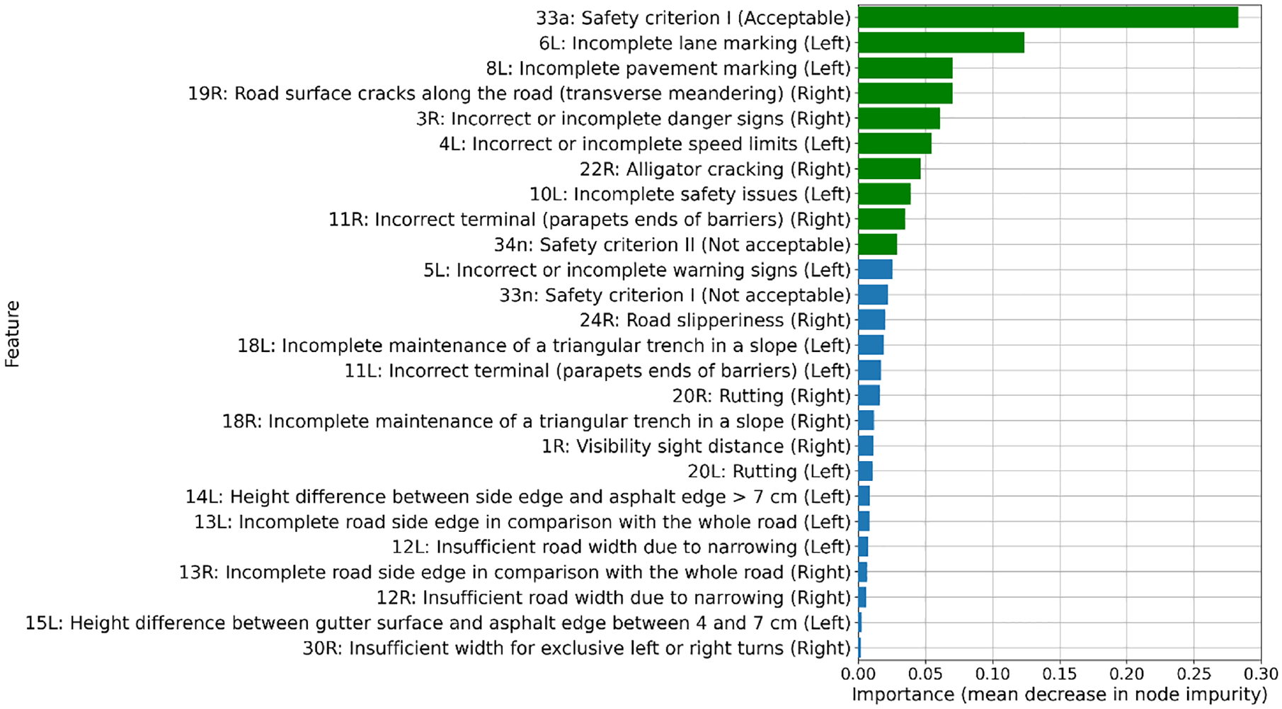
Feature importance based on the extra trees model. The 10 most important features are depicted with green bars.
Overall, geometric design as it pertains to design speed, as well as signage, pavement markings, and pavement condition, were ranked as the most important indicators affecting crash risk. This finding is significant as it allows for informed and cost-effective data collection and maintenance decisions.
Conclusion
This study focused on predicting high crash-risk locations by employing 35 roadway indicators in three ML models. The models were based on the data of the Hellenic National Road Safety Project developed during 2012 to 2015. The database performed in this research included 5,383 locations with 351 of them classified as CCs locations, assumed to be high crash-risk locations identified through the accident analysis approach, and PCCs, assumed to be medium to low crash-risk since this was based on site inspection data, testimonies, and geometrical characteristics. As a result, this dataset constituted an imbalanced dataset, given the big difference in the number of CCs versus PCCs. The original database consisted of 67 roadway features (indicators). However, following a feature engineering process these were finally reduced to 26, which were then used in the ML model training and testing.
Three binary models were developed—random forest, gradient boosting, and extra trees—using oversampling techniques to balance the minority and majority classes. Although all three models performed well, the extra trees model ultimately presented a slightly higher AP value based on the PRCs. Using PRCs for this model, it was estimated that more than 90% of CCs could be detected in new locations, but this led to a conservative approach, since about 60% to 70% of the whole predictions were misclassified.
These prediction results could be modified by changing the probability threshold of the trained model to optimize the appropriate precision–recall relation based on the specifics of the engineering requirements. Thus, it is a question of engineering judgment whether one should follow a conservative path of high recall values to verify actual CC locations at the risk of misclassifying some locations as CCs, or select a high-precision threshold that makes more precise CC predictions, but allows more observations to be misclassified as PCCs. Yet, the F1 score provided a viable method of selecting a threshold that balances both precision and recall.
Another contribution of this study was ranking the roadway features by importance. The majority of the features that scored high included geometric design related to speed as well as lane markings and signage. This finding is important not only because it can inform future data collection efforts to create safety-related roadway inventories, but also for informing cost-efficient maintenance and overall safety intervention activities.
This methodological framework is transferable since it is based on a dataset containing roadway environmental factors typically collected during roadway inventory processes ( 31 ). Given that the models were developed by only accounting for roadway characteristics and not driver behavioral factors or weather-related characteristics, an argument could be made that they could be representative of other locations. That said, differences in how crashes are documented in other countries might have an impact on the transferability of this study’s results.
In summary, this research contributes a methodological framework that can be readily deployed to other locations to predict high crash-risk segments as well as the determination of key roadway features that significantly affect road safety. Further avenues for research might include exploring dimensionality reduction techniques to better analyze the underlying factors affecting road crashes. In addition, future work could consider cost-sensitive- and active learning techniques to improve the model’s performance. Long-term research efforts could also investigate the development of artificial intelligence frameworks that would serve as real-time monitoring systems of roadway conditions and provide recommendations on preemptive repairs on a road segment to reduce the risk of crashes.
Footnotes
Acknowledgements
We acknowledge the invaluable contribution of all professionals involved in the development of the Hellenic National Road Safety Project 2012 to 2015.
Author Contributions
The authors confirm contribution to the paper as follows: study conception and design: D. Sarigiannis, M. Atzemi, J. Oke, E. Christofa, S. Gerasimidis; data collection: M. Atzemi; analysis and interpretation of results: J. Oke, D. Sarigiannis; draft manuscript preparation: D. Sarigiannis; manuscript revision: D. Sarigiannis, J. Oke, E. Christofa. All authors reviewed the results and approved the final version of the manuscript.
Declaration of Conflicting Interests
The authors declared no potential conflicts of interest with respect to the research, authorship, and/or publication of this article.
Funding
The authors received no financial support for the research, authorship, and/or publication of this article.