Novel Speed-Flow Model Based on Queuing Theory and Its Potential Application in Highway Capacity Guidelines

Abstract

Speed-flow relationships are incorporated in many highway capacity guidelines such as the U.S. Highway Capacity Manual (HCM) and the German Highway Capacity Manual (HBS). The speed-flow relationship can be used to predict the operating speed depending on the traffic volume. Based on traffic-flow theory, many models for the speed-flow relationship under fluid and congested traffic conditions have been developed. However, most of the speed-flow relationships used in guidelines are either based on empirical regression analysis and thus lack a theoretical background or include model parameters that do not have a realistic meaning. In this paper, a speed-flow relationship is derived based on the queuing theory in a form that the main model parameters can be expressed as real traffic-flow parameters, which can be obtained by field measurements. These parameters are the free-flow speed, the potential capacity of the imbedded queuing system, and a parameter for the stochastics of the queuing system. By varying the model parameters, different geometric, traffic, and control conditions can be considered. Even the impact of new technologies such as connected and automated vehicles can be accounted for by adjusting those parameters.

Keywords

operations highway capacity and quality of service capacity freeways Highway Capacity Manual (HCM)traffic-flow theory and characteristics car-following

To model the traffic flow characteristics of freeways, the functional relationship between the flow rate q, the speed V, and the density d can be considered in a certain relationship. In practice, the speed-flow relationship is preferred for estimating the speed V depending on the flow rate q. The relationship between q, V, and d can be interlinked by the so-called state equation q = d · V and represented by the Fundamental Diagram. In the literature, many speed-flow models with different levels of sophistication are given. In general, two traffic-flow regimes can be distinguished: (a) the fluid flow regime; and (b) the congested flow regime. The two flow regimes have different characteristics and features. While several speed-flow models are based on useful function types which are fitted to speed-flow data by regression analysis, some models were derived theoretically. For example, the speed-flow relationship in the fluid flow regime can be modeled by applying the queuing theory ( 1 – 3 ), and the speed-flow relationship in the congested flow regime can be modeled by a simple car-following model, namely the Herman’s Rule ( 4 , 5). Correspondingly, the transition area between fluid and congested flow can also be modeled by a single mathematical function so that a continuous Fundamental Diagram can be obtained ( 6 , 7 ). A comprehensive overview of speed-flow models is given by Hall ( 8 ).

In this paper, a novel model for the speed-flow relationship based on the queuing theory is proposed. In the proposed model, microscopic parameters such as the time headway and macroscopic parameters such as the average speed and flow rate can be linked together. Combined with a simple car-following model, the whole speed-flow relationship can also be described by a few basic microscopic parameters.

For applications in traffic engineering, the speed-flow relationships in fluid and congested flow are usually treated separately ( 9 , 10 ). Thus, in the applications presented in this paper, the congested flow regime is not considered explicitly because it is usually not relevant for highway planning and design projects.

In the following section, the proposed model is formulated. Thereafter, different conventions for defining the capacity of freeways are discussed. Example applications of the proposed model representing the speed-flow relationships for basic freeway segments given in the German Highway Capacity Manual HBS ( 9 ) and in the U.S. HCM ( 10 ) are presented. Finally, the relationships between macroscopic and microscopic traffic-flow parameters are discussed and some conclusions are drawn.

Proposed Model Formulation for the Speed-Flow Relationship

Fluid Traffic Flow (Including Partially Bunched Flow)

We consider a cross section (see Figure 1, cross section A) of a motorway segment and a vehicle just behind this cross section. If there are no other vehicles downstream traveling within the interaction area of length L₀ = τ·V_FF (from A to B), where τ is the minimum gross time headway (from rear-bumper to rear-bumper) between two consecutively following vehicles and V_FF is the free-flow speed (desired speed) of the considered vehicle, the considered vehicle can travel though the interaction area without being influenced by a vehicle in front.

Figure 1.

Length of the interaction area L₀ = τ·V_FF between two consecutive vehicles.

The minimum gross time headway τ corresponds to the reciprocal of the potential cross-section capacity C₀ under fluid flow conditions. However, the potential capacity C₀ of the considered cross section cannot be observed directly in the field because the traffic flow may break down before reaching this potential capacity, leading to a change from fluid to congested flow conditions. The potential capacity is a random parameter which can only be determined by statistical methods for censored data (Censored Data Method [CDM]) like the Product-Limit Method (PLM) or the Maximum-Likelihood estimation technique ( 11 – 15 ). Using these methods, the probability distribution function (PDF) and subsequently the mean value of the potential capacity C₀ can be estimated. The mean value of the potential capacity C₀ corresponds to the reciprocal of the average gross time headway of bunched vehicles traveling in a platoon. In general, the average potential capacity C₀ also depends on the aggregation interval of the observed data. Generally, single-vehicle data can be used for the parameter estimation; however, these are rarely available. If aggregated data are used, a short interval length (e.g., 1 min or 5 min) should be selected. If single-vehicle data are available, the average gross time headway τ within platoons can be used directly to estimate the average potential capacity C₀. The average potential capacity C₀ is the reciprocal of the average time headway τ. The PDF and the mean value of C₀ can be obtained directly from the PDF and the mean value of τ. The potential capacity C₀ can be described as a Weibull-distributed random variable. The Weibull distribution is typically used for hazard probability estimations. It fits well to the capacity estimation by defining the event of the flow rate exceeding the capacity as a hazard event ( 13 – 15 ).

In Figure 2, an example of the measured speed-flow data of a two-lane motorway carriageway and the estimated Weibull distribution function of the potential capacity with β = 4,448 vehicles per hour (vph), α = 18.4, and C₀ = 4,321 vph is illustrated.

Figure 2.

Example of measured speed-flow data and estimated Weibull capacity distribution with a mean of C₀ = 4,321 vehicles per hour (vph) of the two-lane carriageway of freeway A43 between Bochum-Riemke and Bochum-Gerthe, Germany.

The mean value of the potential capacity C₀ corresponds to the highest measured flow rates. This fact shows again that the mean potential capacity C₀ estimated by the CDM is the ideal capacity of the imbedded queuing system, which is rarely reached in reality.

The considered cross section A can be treated as a service counter in a G/G/1 queuing system. The waiting time t_w of the queuing system can be calculated based on queuing theory. Then, the time headway between two consecutively following vehicles, that is, the average cruising time through the interaction area of length L₀, is

Δ t_{fluid} = τ_{fluid} + t_{w} = \frac{L_{0}}{V_{FF}} + t_{w}

(1)

where

t_w = $\frac{x^{2}}{q \cdot (1 - x)} \cdot k_{st} = \frac{x}{C_{0} \cdot (1 - x)} \cdot k_{st}$

= waiting time in the queue of a G/G/1 queuing system (h),

x = $\frac{q}{C_{0}}$ = degree of saturation of the queuing system,

C ₀ = mean potential capacity of the queuing system (vph),

k_st = factor accounting for the stochastic property of the queuing system,

τ_fluid = 1/C₀ = mean minimum gross time headway at V = V_FF under fluid flow conditions (h),

V_FF = free-flow speed (km/h),

L ₀ = length of the interaction area (km).

Assuming a G/G/1 queue is an approximation. However, the G/G/1 queue is the best and simplest model to represent the queuing system in a generalized bottleneck analysis where the characteristics of arrivals and departures can be described by a general distribution function. A G/G/1 queue is a general assumption covering almost all types of queuing system, such as the M/M/1 queue, M/D/1 queue, and others. Different road types, which may incorporate different microscopic driver behaviors, can also be accounted for with the proposed model.

The common time unit in traffic engineering applications is one hour (h), not one second (s). Therefore, the time unit of one hour is also used for the time headway and the waiting time to avoid unnecessary transformations of the parameter units.

The parameter τ_fluid is the mean minimum gross time headway over all traffic lanes under fluid flow conditions at V = V_FF. It can be calculated as:

τ_{fluid} = \frac{1}{n} \cdot (t_{0, fluid} + \frac{l_{veh}}{V_{FF}})

(2)

where

l_veh = standstill distance between two vehicles (km),

t _0,fluid = mean minimum net time headway (from real-bumper to front-bumper) between two consecutive vehicles in platoons under fluid flow conditions (h)

= mean reaction time + buffer time ≈ 1.2–1.5 s,

n = number of lanes.

The mean values of the potential capacity of the considered queuing system can be obtained from Equation 2. That is,

C_{0} = \frac{1}{τ_{fluid}} = \frac{n}{t_{0, fluid} + \frac{l_{veh}}{V_{FF}}}

(3)

The parameter k_st depends on the stochastic properties of the inflow (corresponding to the traffic demand flow rate) and the maximum outflow (corresponding to the cross-section capacity) of the queuing system. With increasing flow rate, the value of k_st decreases because of the higher proportion of bunched vehicles. If the variances of the inflow and the maximum outflow are known, the exact value of k_st can be computationally obtained ( 16 , 17 ). For simplification, a small value of k_st at higher flow rates is used for all flow rates q in the paper. The resulting deviation in the calculation of the waiting time t_w is small and considered negligible because at lower flow rates the waiting time is always very small and thus the influence of flow variance is not significant. The value of k_st can be calibrated against field measurements. On average, the value of k_st is between 0.01 and 0.12 for level freeway segments. This value seems to be very small but is realistic because the service time (the reciprocal of the mean potential capacity C₀) and the intra-arrival time at a high flow rate (the reciprocal of the flow rate q) are nearly deterministic for the embedded queuing system. For uphill segments, the value of k_st is larger because the traffic flow becomes more inhomogeneous reflecting different vehicle acceleration capabilities.

Thus, the actual speed V through the interaction area L₀ can be given as a function of the flow rate q:

V (q)_{fluid} = \frac{L_{0}}{Δ t} = \frac{τ_{fluid} \cdot V_{FF}}{τ_{fluid} + t_{w} (q)} = \frac{V_{FF}}{1 + \frac{t_{w} (q)}{τ_{fluid}}}

(4)

Inserting $τ_{fluid} = 1 / C_{0}$ and $t_{w} = \frac{x}{C_{0} \cdot (1 - x)} \cdot k_{st}$ yields

V (q)_{fluid} = \frac{V_{FF}}{1 + \frac{\frac{x}{C_{0} \cdot (1 - x)} \cdot k_{st}}{1 / C_{0}}} = \frac{V_{FF}}{1 + \frac{x}{1 - x} \cdot k_{st}} = \frac{V_{FF}}{1 + \frac{q}{C_{0} - q} \cdot k_{st}}

(5)

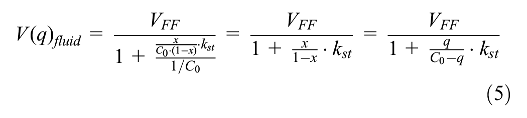
This equation satisfies the necessary boundary conditions of V = V_FF at q = 0 and V = 0 at q = C₀.

From Equation 5, the speed-flow relationship for fluid flow conditions becomes

q (V)_{fluid} = \frac{C_{0}}{\frac{k_{st} V}{V - V_{FF}} + 1}

(6)

In fluid traffic flow, the average time headway is then:

h_{fluid} = \frac{1}{q} = \frac{1}{C_{0}} \cdot (\frac{k_{st} V}{V - V_{FF}} + 1)

(7)

By varying the parameters k_st, V_FF, and C₀, all measurements in fluid traffic can be represented by Equation 5. Thus, the distribution of those parameters and, therefore, the random nature of the traffic flow can be considered by the proposed model very well. In Figure 3, the speed-flow relationships from Equation 5 with different variations of the parameters k_st, V_FF, and C₀ are illustrated. A very good representation of all measurements can be obtained for the whole range of fluid flow conditions up to the transition area into congested flow. The parameters k_st, V_FF, and C₀ (depending on the vehicle length and reaction time, cf. Equation 3) can also be given as functions of the grade s and the proportion of heavy vehicles.

Figure 3.

Speed-flow relationships in fluid traffic flow for different values of (a) k_st, (b) V_FF, and (c) C₀ together with empirical data from the two-lane carriageway of freeway A43 between Bochum-Riemke and Bochum-Gerthe, Germany.

Congested Traffic Flow

Equation 5 is only valid for fluid traffic flow under the limitation of Equation 1 that there is only one vehicle in the interaction area (cf. Figure 1). If this limitation is exceeded, the average time headway between two consecutive vehicles is smaller than the cruising time in the interaction area of length L₀. On average, there is more than one vehicle within the interaction area so that the presumption for Equation 1 is no longer valid. The traffic state changes from fluid to congested flow where other characteristics must be considered.

In congested flow, all vehicles follow each other with a mean time headway as follows (Herman’s Rule [4]):

h_{cong} = \frac{1}{n} (t_{0, cong} + \frac{l_{veh}}{V})

(8)

where t_0,cong = mean minimum net time headway in congested flow (h).

Traffic flow changes from fluid into congested conditions at h_fluid = h_cong. That is, the value of Equation 7 is equal to the value of Equation 8.

In congested flow, the average distance between consecutive vehicles is:

Δ X = V \cdot h_{cong} = \frac{1}{n} \cdot (t_{0, cong} V + l_{veh})

(9)

That is,

\begin{matrix} d = \frac{1}{Δ t} = \frac{1}{\frac{1}{n} \cdot (t_{0, cong} \cdot V + l_{veh})} = \frac{1}{\frac{t_{0, cong}}{n} \cdot \frac{q}{d} + \frac{l_{veh}}{n}} \\ = \frac{1}{\frac{t_{0, cong}}{n} \cdot \frac{q}{d} + \frac{1}{d_{max}}} \end{matrix}

(10)

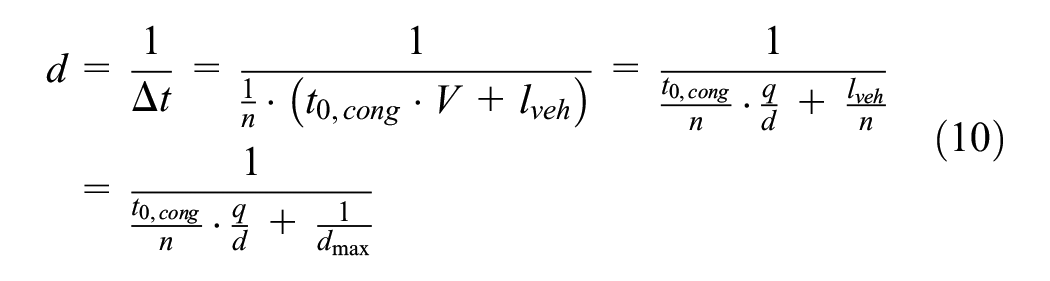
Solving this equation toward the flow rate q yields

q = \frac{n}{t_{0, cong}} \cdot (1 - \frac{d}{d_{max}}) = K_{0} \cdot (1 - \frac{d}{d_{max}})

(11)

where

d_max = n/l_veh = maximum density of standstill traffic (veh/km)

K ₀ = n/t_0,cong (vph)

The corresponding speed is:

V (q)_{cong} = \frac{1}{d_{max} \cdot (\frac{1}{q} - \frac{1}{K_{0}})}

(12)

In Figure 4, the shape of Equation 12 with different values of t_0,cong is illustrated. Again, the measurements in congested flow can be represented very well. The parameter t_0,cong can be given as a function of the grade s and of the proportion of heavy vehicles as well.

Figure 4.

Speed-flow relationships in congested flow for different values of t_0,cong.

Depicting the speed-flow curves according to Equations 5 and 12 together with measured data, all measurements in both fluid and congested flow can be represented by varying the model parameters (Figure 5).

Figure 5.

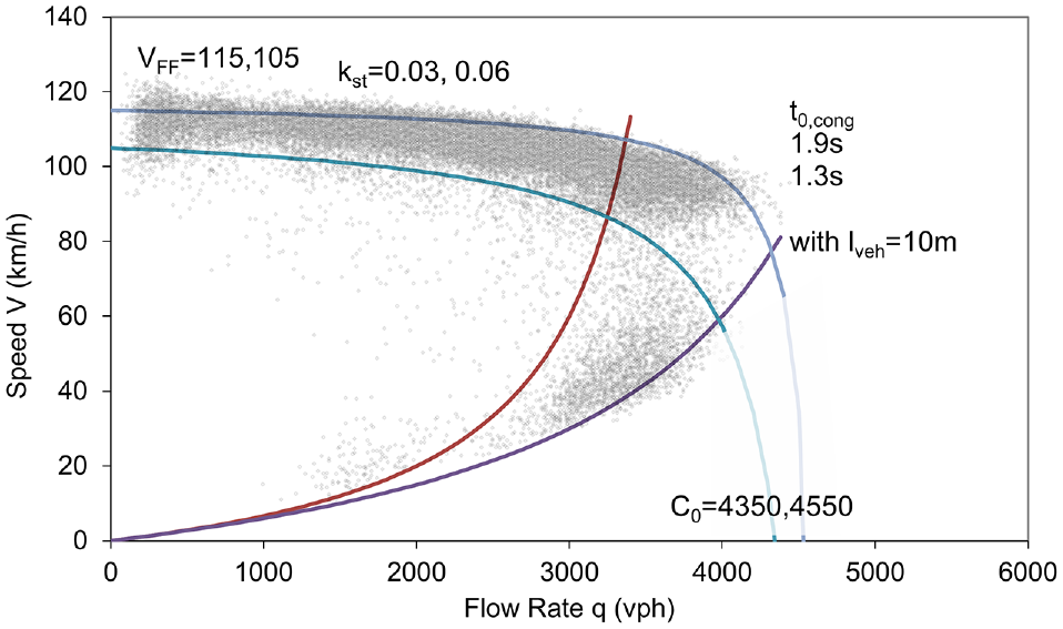
Outlines of the speed-flow relationships in fluid and congested flow.

It can be concluded that the measured speed-flow data can be represented by two general functions, one for fluid flow and one for congested flow. All measured data are within the boundaries using k_st = 0, q = C₀, l_veh = 0, and d_max = 1/l_veh = ∞ (Figure 6). The maximum volume, which can be used as a fixed-value estimate of the capacity q_max for practical applications, can be obtained at the intersection of the speed-flow relationships for fluid and congested flow. Under this consideration, the capacity q_max is a function of the parameters V_FF, C₀, k_st, l_veh, and t₀. The mean minimum net time headway t₀ can be different for the fluid and congested flow regimes. Normally, in congested flow, the average value of t_0,cong is larger than the average value of t_0,fluid in fluid flow because of stronger acceleration and deceleration in stop-and-go traffic. The maximum possible capacity is reached at k_st = 0. The considered queuing system is then totally deterministic. For t_0,cong = t_0,fluid, the queuing system has the capacity q_max,_cong = q_max,_fluid = C₀ at k_st = 0.

Figure 6.

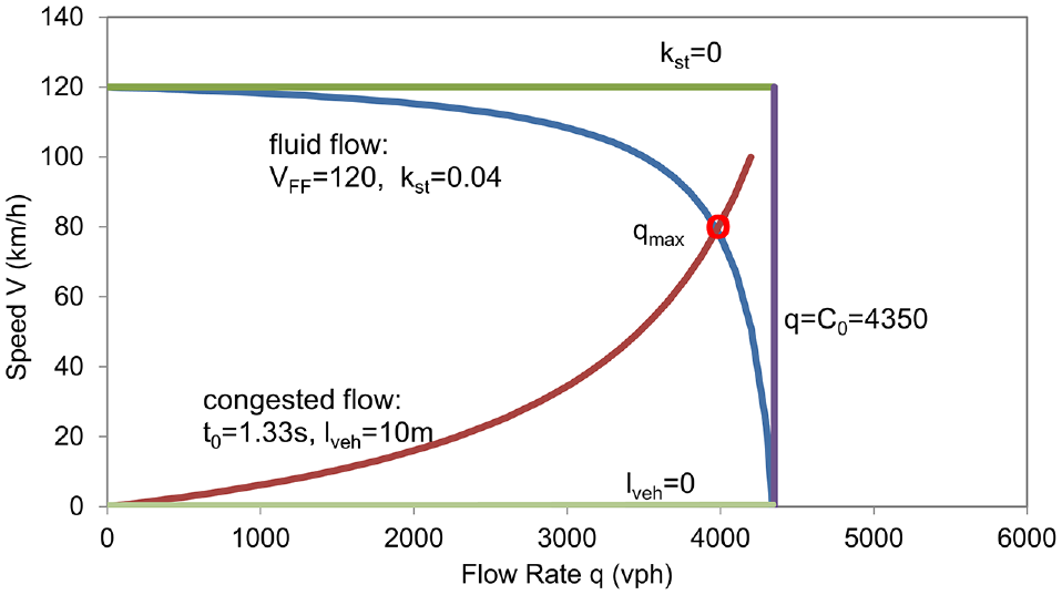
Boundaries of the speed-flow relationship (with C₀ = 4,350 vehicles per hour [vph] and t_0,cong = t_0,fluid).

Conventions for Determining the Capacity

A fixed-value estimate of the capacity can be determined according to different criteria and conventions. For example, the capacity can be defined by the intersection of the speed-flow relationships for fluid and congested flow. Usually, a predefined critical speed V_crit ( 9 ) or a predefined critical density d_crit ( 10 ) is used to determine the capacity. Therefore, the capacity can be different in different guidelines.

Capacity as the Flow Rate at the Intersection of the Speed-Flow Relationships for Fluid and Congested Flow

The flow rate and speed at the intersection of the speed-flow relationships for fluid flow (Equation 5) and congested flow flow (Equation 12) can be regarded as fixed-value estimates of the capacity q_max and the critical speed V_crit at capacity, respectively. That is, we postulate:

V (q)_{fluid} = V (q)_{cong} \Rightarrow \frac{V_{FF}}{1 + \frac{q}{C_{0} - q} \cdot k_{st}} = \frac{1}{(\frac{1}{q} - \frac{1}{K_{0}}) \cdot d_{max}}

(13)

This is a quadratic function of q. Solving this function toward q yields

q_{max} = \frac{b - \sqrt{b^{2} - 4 ac}}{2 a}

(14)

where

\begin{matrix} a = V_{FF} \cdot d_{max} + K_{0} \cdot (1 - k_{st}) \\ b = V_{FF} \cdot d_{max} \cdot (C_{0} + K_{0}) + C_{0} \cdot K_{0} \\ c = C_{0} \cdot K_{0} \cdot V_{FF} \cdot d_{max} \end{matrix}

(14)

The corresponding critical speed at capacity q_max is:

V_{crit} = \frac{V_{FF}}{1 + \frac{q_{max}}{C_{0} - q_{max}} \cdot k_{st}}

(15)

Capacity as the Flow Rate at a Predefined Critical Speed V_crit

Solving Equation 5 toward q with V = V_crit yields

q_{max} = C_{0} \cdot \frac{1}{1 + \frac{k_{st} \cdot V_{crit}}{V_{FF} - V_{crit}}}

(16)

Capacity as the Flow Rate at a Predefined Critical Density d_crit

From Equation 5, the density d is

d = \frac{q}{V} = \frac{1 + \frac{q}{C_{0} - q} \cdot k_{st}}{V_{FF}} q

(17)

Therefore, the critical density d_crit at capacity is

d_{crit} = \frac{1 + \frac{q_{max}}{C_{0} - q_{max}} k_{st}}{V_{FF}} q_{max}

(18)

The solution toward q_max is:

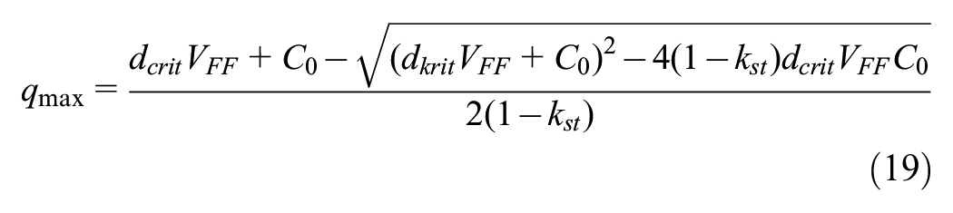
q_{max} = \frac{d_{crit} V_{FF} + C_{0} - \sqrt{{(d_{krit} V_{FF} + C_{0})}^{2} - 4 (1 - k_{st}) d_{crit} V_{FF} C_{0}}}{2 (1 - k_{st})}

(19)

In Table 1, the capacity values for the same model parameters but different capacity definitions together with the corresponding values of V_crit and d_crit are given.

Table 1.

Capacity Values for the Example Cross Section of a Two-Lane Carriageway with the Model Parameters V_FF = 113 km/h, C₀ = 4,300 vph, k_st = 0.03, and l_veh = 10 m

	Capacity q_max (vph)	V_crit (km/h)	d_crit (vph)
Intersection V_fluid = V_cong	4,025	78.49	51.29
Predefined V_crit = 70 km/h	4,100	70	58.57
Predefined V_crit = 80 km/h	4,008	80	50.11
Predefined d_crit = 60 veh/km	4,110	68.50	60
Predefined d_crit = 50 veh/km	4,007	80.14	50

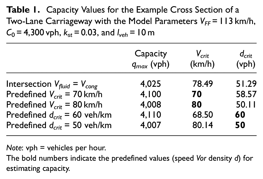
Note: vph = vehicles per hour.

The bold numbers indicate the predefined values (speed Vor density d) for estimating capacity.

Applications of the New Model

As a first application, the proposed speed-flow model can be fitted to the speed-flow relationships for basic freeway segments given in the HBS ( 9 ) and the HCM ( 10 ). As mentioned above, only the fluid flow regime is considered here.

HBS Model

In the HBS ( 9 ), the speed-flow model from Brilon and Ponzlet ( 1 ) is incorporated. This model was derived under the assumptions of an M/M/1 queuing system (i.e., with k_st = 1) and the length of the interaction area being independent of the free-flow speed (L₀≠τ·V_FF). The speed-flow relationship in the HBS ( 9 ) is given by

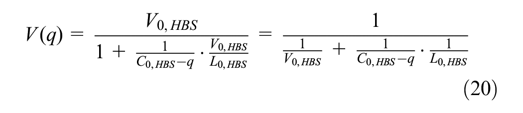
V (q) = \frac{V_{0, HBS}}{1 + \frac{1}{C_{0, HBS} - q} \cdot \frac{V_{0, HBS}}{L_{0, HBS}}} = \frac{1}{\frac{1}{V_{0, HBS}} + \frac{1}{C_{0, HBS} - q} \cdot \frac{1}{L_{0, HBS}}}

(20)

where V_0,HBS, C_0,HBS, and L_0,HBS are model parameters, which are labeled with the index “HBS” to be distinguishable from the parameters of the newly derived model.

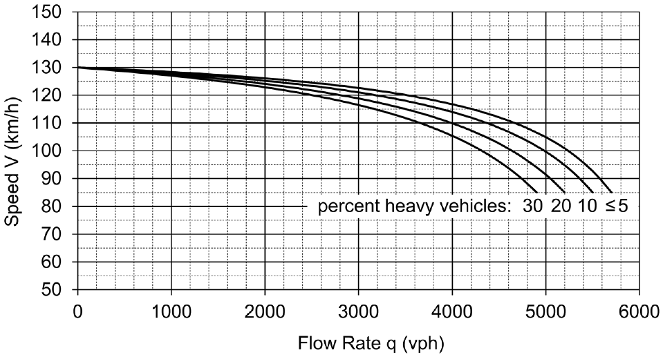
The HBS ( 9 ) procedure for the quality-of-service assessment of basic freeway segments includes speed-flow diagrams and corresponding parameters for two-, three-, and four-lane carriageways in rural and urban areas with different grades, heavy vehicle percentages, and speed limits. As an example, Figure 7 shows the speed-flow diagrams for three-lane carriageways in urban areas with no speed limit and a longitudinal gradient below 2% for different heavy vehicle percentages. Note that the HBS ( 9 ) procedure uses total flow rates of the whole carriageway instead of per-lane flow rates as a result of the rather uneven lane-flow distribution on German freeways.

Figure 7.

HBS ( 9 ) speed-flow relationships for three-lane freeway carriageways in level terrain within urban areas for different heavy vehicle percentages ( 12 ).

Given the unreasonable presumptions mentioned above, the model parameters V_0,HBS and L_0,HBS are not compatible with the corresponding measurable values in the field. In any event, Equation 20 includes the same number of parameters as Equation 5. Both equations can be transformed into an identical structure. Thus, the parameters are interrelated and can be mathematically transformed into each other.

For Equation 5, the values of C_0,HBS can be inherited directly. Equation 5 can be rewritten as:

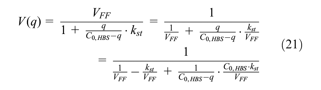
\begin{matrix} V (q) = \frac{V_{FF}}{1 + \frac{q}{C_{0, HBS} - q} \cdot k_{st}} = \frac{1}{\frac{1}{V_{FF}} + \frac{q}{C_{0, HBS} - q} \cdot \frac{k_{st}}{V_{FF}}} \\ = \frac{1}{\frac{1}{V_{FF}} - \frac{k_{st}}{V_{FF}} + \frac{1}{C_{0, HBS} - q} \cdot \frac{C_{0, HBS} \cdot k_{st}}{V_{FF}}} \end{matrix}

(21)

Comparing the denominators of both Equations 5 and 20 yields

V_{FF} = \frac{1}{\frac{1}{V_{0, HBS}} + \frac{1}{L_{0, HBS} \cdot C_{0, HBS}}}

(22)

and

k_{st} = \frac{1}{\frac{L_{0, HBS} C_{0, HBS}}{V_{0, HBS}} + 1}

(23)

Therefore, the parameters of the HBS ( 9 ) model can be partially inherited directly (q_max, C₀, and V_crit) and partially transformed into the new parameters (V_FF and k_st) under the condition that Equation 5 delivers the same capacity q_max and the same critical speed V_crit (cf. Equation 20). The model parameters V_FF and k_st then describe exactly the free-flow speed and the stochastic property of the imbedded queuing system.

In Table 2, parameters for Equation 5 transformed from selected speed-flow relationships given in the HBS ( 9 ) are provided.

Table 2.

Parameters of Equation 5 for Three-Lane Basic Freeway Segments without Speed Limit Depending on the Grade, the Heavy Vehicle Percentage, and the Location of the Freeway in Rural or Urban Areas according to the HBS ( 9 )

Grade	≤ 2%				3%				4%				5%
% heavy vehicles	≤ 5%	10%	20%	30%	≤ 5%	10%	20%	30%	≤ 5%	10%	20%	30%	≤ 5%	10%	20%	30%
Rural areas
V_FF	139	139	139	139	137	137	137	137	134	134	134	134	128	128	128	128
k_st	0.0785	0.0867	0.1052	0.1214	0.1018	0.1098	0.1320	0.1516	0.1258	0.1381	0.1676	0.1936	0.1540	0.1707	0.2068	0.2381
C ₀	6,064	6,028	5,846	5,626	6,065	6,015	5,836	5,615	5,813	5,781	5,617	5,404	5,481	5,463	5,300	5,080
q_max	5,300	5,200	4,900	4,600	5,200	5,100	4,800	4,500	4,900	4,800	4,500	4,200	4,500	4,400	4,100	3,800
V_crit	90	90	90	90	85	85	85	85	80	80	80	80	75	75	75	75
Urban areas
V_FF	130	130	130	130	128	128	128	128	125	125	125	125	120	120	120	120
k_st	0.0694	0.0832	0.0998	0.1146	0.0849	0.0982	0.1194	0.1384	0.1027	0.1204	0.1506	0.1777	0.1247	0.1520	0.1845	0.2128
C ₀	6,448	6,365	6,180	5,961	6,392	6,284	6,115	5,907	6,117	6,021	5,885	5,700	5,755	5,700	5,536	5,321
q_max	5,700	5,500	5,200	4,900	5,600	5,400	5,100	4,800	5,300	5,100	4,800	4,500	4,900	4,700	4,400	4,100
V_crit	85	85	85	85	80	80	80	80	75	75	75	75	70	70	70	70

In Figure 8, the transformed parameters k_st for the motorway segment types given in Table 2 are compared. It can be seen that the parameter k_st represents the flow homogeneity. The smaller the value of k_st, the more homogeneous the traffic flow. With the increasing proportion of heavy vehicles and the increasing grade, the value of k_st increases as well. The speed-flow relationships of motorway segments located in urban areas are always represented by a smaller value of k_st compared with rural motorways. Both effects reflect field observations very well.

Figure 8.

Values of k_st for different types of three-lane freeway segments without speed limit.

The speed-flow relationships in the HBS are well calibrated with German freeway data. Thus, the proposed model (Equation 5), which delivers the same speed-flow curve as the HBS model (Equation 20), fits German freeway data very well.

HCM Model

Brilon and Lohoff ( 2 ) already attempted to fit Equation 20 to the HCM ( 10 ) speed-flow curves for basic freeway segments. However, because the parameters in Equation 20 do not have realistic meanings, the resulting model parameters cannot be associated with the free-flow speed and the capacity. Instead, the new proposed model includes the free-flow speed and the capacity as model parameters and can be fitted to the HCM speed-flow relationships by only calibrating k_st. In Figure 9, the fitted model curves and the HCM speed-flow relationships are illustrated together. The HCM speed-flow curves consist of two parts: a horizontal line V = FFS (=V_FF) for lower flow rates and one quadratic function for higher flow rates, whereas the curves according to Equation 5 have a steadily increasing slope and therefore consider a slight decrease of the speed with increasing flow rate at low and moderate traffic flow rates. The corresponding parameters C₀ and k_st are given in Table 3. In this experiment, the values of C₀ are chosen to be 1.1 times the capacity c. The capacities c and the free-flow speeds FFS according to the HCM ( 10 ) are exactly maintained. Note, in the HCM, the unit passenger-car equivalents in passenger car (pc) is used for flow rate q and capacity c in place of the unit vehicles (veh). Thus, in the HCM the flow rate q and the capacity c have the unit pcphpl (Passenger-car equivalents in passenger car per hour per lane) in place of vphpl.

Figure 9.

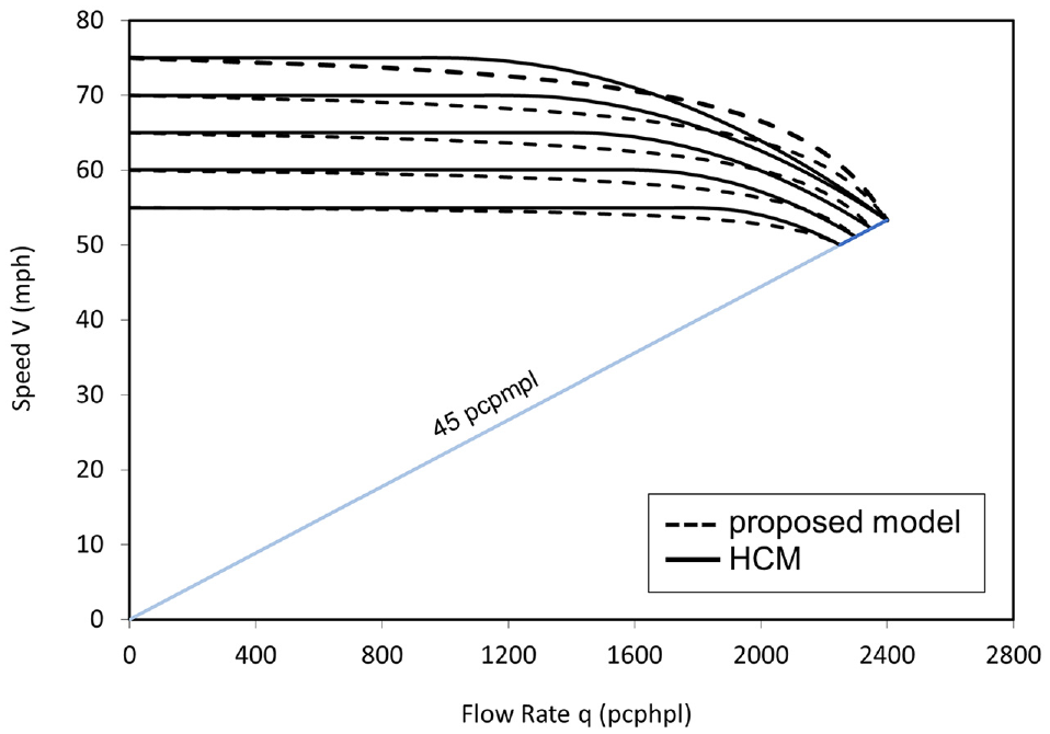
Proposed model fitted to the speed-flow relationships for basic freeway segments given in the HCM ( 10 ).

Table 3.

Parameters for Equation 5 for the Speed-Flow Relationships of Basic Freeway Segments Given in the HCM ( 10 )

	FFS (mph)
	75	70	65	60	55
C ₀ (pcphpl)	2,640	2,640	2,585	2,530	2,475
k_st	0.041	0.031	0.024	0.017	0.01
c (pcphpl)	2,400	2,400	2,350	2,300	2,250
V_crit (mph)	53.33	53.33	52.22	51.11	50
C ₀ /c	1.1	1.1	1.1	1.1	1.1

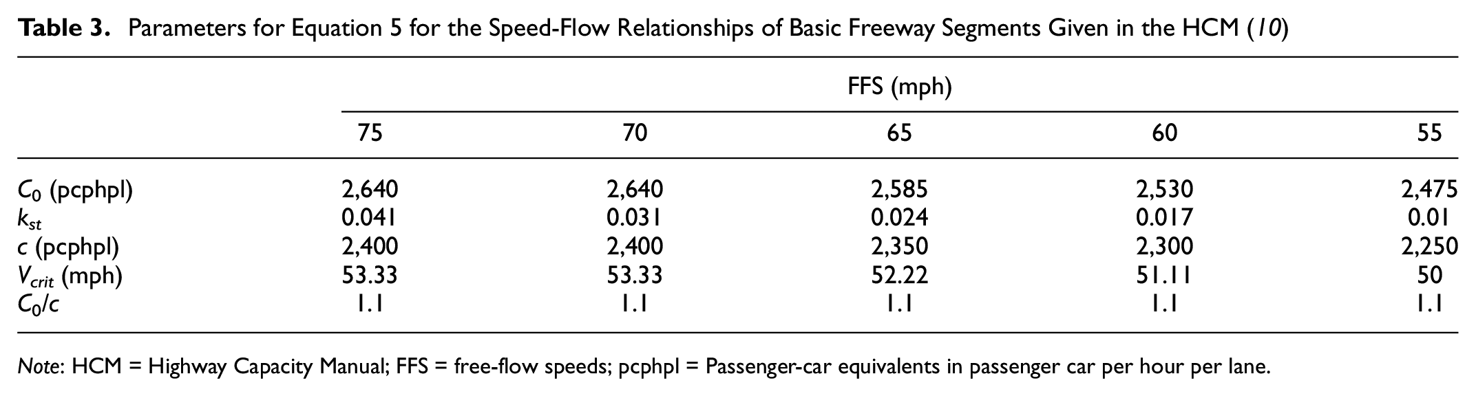
Note: HCM = Highway Capacity Manual; FFS = free-flow speeds; pcphpl = Passenger-car equivalents in passenger car per hour per lane.

In Table 3, the values of FFS, V_crit and c (= q_max) are inherited directly from the HCM ( 10 ). The values of k_st can be calibrated by fitting Equation 5 to the HCM speed-flow relationships. Compared with the values of the parameter k_st for German freeways in Table 2, the values of the parameter k_st fitted to the HCM speed-flow curves are much smaller. This indicates that the traffic flow on freeways in the U.S. is more homogenous than in Germany where a lower speed limit of 80 km/h for heavy vehicles and no general speed limited for passenger cars apply.

In Figure 10, the proposed model is illustrated together with the original data, which were used for establishing the HCM speed-flow relationships (cf. [18]). The data were collected at nine sites with FFS = 75 mph, 23 sites with FFS = 70 mph, 14 sites with FFS = 65 mph, and two sites with FFS = 60 mph across nine different states. Neither the HCM model nor the proposed model fit the measurement data perfectly. However, the proposed model, which incorporates a continuous decrease of the speed with increasing flow rate, delivers a slightly more consistent representation of the data in the fluid flow regime than the two-part HCM model.

Figure 10.

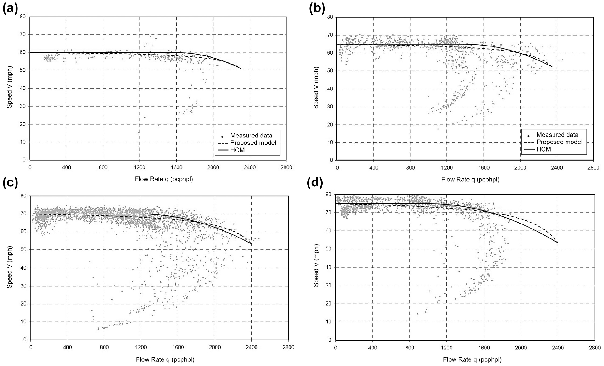
Proposed model compared with the HCM speed-flow relationships and the original data (extracted from Fig.1 in [18]) for different free-flow speeds (FFS): (a) FFS = 60 mph; (b) FFS = 65 mph; (c) FFS = 70 mph; (d) FFS = 75 mph.

Discussion

The derivation of the proposed model is based on the G/G/1 queuing model. A G/G/1 queue is a general assumption with very few limitations, which covers almost all types of queuing system. The parameters of the assumed G/G/1 queue can be calibrated with field data to represent speed-flow relationships for freeways and multilane highways with different geometric, traffic, and control conditions.

Basically, in fluid flow, the parameters V_FF, C₀, and k_st in Equation 5 can be calibrated with single-vehicle data. The three parameters can be determined for all combinations of segment types, gradients, speed limits, and proportions of heavy vehicles. The value of V_FF is the average speed of free-flowing vehicles. The value of C₀ corresponds to the reciprocal of the average gross time headway with bunched platoons. The value of k_st can be obtained from the PDF of the time headways in the inflow (demand) and in the platoons.

To model congested flow, only two model parameters, K₀ = 1/t₀ and d_max = n/l_veh, are required. The values of t₀ and l_veh can be determined from single-vehicle data for all combinations of segment types, gradients, speed limits, and proportions of heavy vehicles.

By regression analysis, the model parameters mentioned above can also be estimated from aggregated data (e.g., data from permanent counting stations). In this way, a relationship between microscopic (single vehicle) and macroscopic (aggregated) data can be established.

From Equations 14, 16, and 19, the often observed capacity increase through an implementation of static or variable speed limits can plausibly be explained by the effect of harmonization (smaller values of k_st). However, for constant values of k_st, a speed limit can lead to a reduction of the capacity. This knowledge can be important for work zone management.

The capacities obtained from queuing theory are approximately inversely proportional to the mean value of the net time headway t₀ and the stochastics of the imbedded queuing system, which is represented by the parameter k_st. For connected and automated vehicles (CAVs), the net time headway t₀ is significantly smaller because of the reduced reaction time. Therefore, in a platoon of CAVs, the driving behavior is more harmonized. In the speed-flow model, this leads to a smaller value of the parameter k_st and thus an additional increase in the capacity. The extent of the capacity increase can be qualified by varying both parameters and the penetration rate of CAVs (cf. [ 19 ]).

Implementing the proposed speed-flow model in traffic management applications can affect the decision-making process with respect to the capacity and travel-time estimation. Because the proposed model is based on the queuing theory, it is in general a stochastic model. Although the proposed speed-flow relationship represents only the average speed and flow rate, the stochastic nature of the capacity and speed can be accounted for by considering the distribution of the waiting time in Equation 1 and its parameters.

The proposed macroscopic speed-flow model is developed from a microscopic model. All effects of microscopic maneuvers are considered in the queuing process globally by the model parameters, especially the parameter k_st. For example, the capacity impact of lane changes can be included using the model parameters.

Summary and Conclusions

A novel formulation of the speed-flow relationship was derived based on queuing theory. The model parameters V_FF (free-flow speed), k_st (stochastics of the queuing system), and C₀ (potential capacity) have physical meanings and can thus be obtained from field measurements. The speed-flow model can be applied to describe traffic flow on basic freeway segments. For this, the values of V_FF, k_st, and C₀ can be given depending on the prevailing geometric, traffic, and control conditions.

As a first application, the proposed new model was fitted to the speed-flow relationships for basic freeway segments given in the HBS and HCM. In the new model, microscopic and macroscopic flow parameters can be linked in a way that both types of flow parameters can be verified with field data.

In future investigations, the model parameters can be recalibrated for specific geometric, traffic, control, and vehicular conditions. Even the impact of new technologies such as CAVs can be accounted for.

Footnotes

Author Contributions

The authors confirm contribution to the paper as follows: study conception and design: Ning Wu, Justin Geistefeldt; data collection: Ning Wu, Justin Geistefeldt; analysis and interpretation of results: Ning Wu, Justin Geistefeldt; draft manuscript preparation: Ning Wu, Justin Geistefeldt. All authors reviewed the results and approved the final version of the manuscript.

Declaration of Conflicting Interests

The author(s) declared no potential conflicts of interest with respect to the research, authorship, and/or publication of this article.

Funding

The author(s) received no financial support for the research, authorship, and/or publication of this article.

ORCID iDs

Ning Wu

Justin Geistefeldt

References

Brilon

Ponzlet

Application of Traffic Flow Models. Proc., Workshop in Traffic and Granular Flow, World Scientific, Singapore, 1995, pp. 23–24.

Brilon

Lohoff

Speed-Flow Models for Freeways. Proc., 6th International Symposium on Highway Capacity and Quality of Service, Stockholm, Sweden, Elsevier, Amsterdam, The Netherlands, 2011, pp. 26–36.

Heidemann

A Queueing Theory Approach to Speed-Flow-Density Relationships. Proc., 3th International Symposium on Transportation and Traffic Theory, Lyon, France, Oxford, UK, 1996, pp. 103–118.

Herman

Prigogine

A Two Fluid Approach to Town Traffic. Science, Vol. 204, 1979, pp. 148–151.

A New Approach for Modeling of Fundamental Diagrams and Its Applications. Transportation Research Part A: Policy and Practice, Vol. 36, No. 10, 2002, pp. 867–884.

Van Aerde

. Single Regime Speed-Flow-Density Relationship for Congested and Uncongested Highways. Proc., 74th TRB Annual Conference, Washington DC, 27 January 1995, Paper No. 950802.

Rakha

Derivation of the van Aerde Traffic Stream Model from Tandem-Queueing Theory. Transportation Research Record: Journal of the Transportation Research Board, 2009. 2124: 18–27.

Hall

Traffic Stream Characteristics. In: Traffic Flow Theory. A State-of-the-Art Report. Transportation Research Board, Committee on Traffic Flow Theory and Characteristics, Washington, D.C., 2001.

FGSV. Handbuch für die Bemessung von Straßenverkehrsanlagen—HBS 2015 (German Highway Capacity Manual). German Road and Transportation Research Association (FGSV), Cologne, 2015.

10.

TRB. Highway Capacity Manual (HCM), 7th Edition. Transportation Research Board, The National Academic Press, Washington, D.C., 2022.

11.

Brilon

Ponzlet

Variability of Speed-Flow Relationships on German Autobahns. Transportation Research Record: Journal of the Transportation Research Board, 1996. 1555: 91–98.

12.

Geistefeldt

Assessment of Basic Freeway Segments in the German Highway Capacity Manual HBS 2015 and Beyond. Transportation Research Procedia, Vol. 15, 2016, pp. 417–425.

13.

Brilon

Geistefeldt

Regler

Reliability of Freeway Traffic Flow: A Stochastic Concept of Capacity. Proc., 16th International Symposium on Transportation and Traffic Theory, College Park, MD, Elsevier, New York, 2005, pp. 125–144.

14.

Brilon

Geistefeldt

Zurlinden

Implementing the Concept of Reliability for Highway Capacity Analysis. Transportation Research Record: Journal of the Transportation Research Board, 2007. 2027: 1–8.

15.

Geistefeldt

Brilon

A Comparative Assessment of Stochastic Capacity Estimation Methods. Proc., 18th International Symposium on Transportation and Traffic Theory, Transportation and Traffic Theory 2009: Golden Jubilee, Springer, Dordrecht, Heidelberg, London, New York, 2009, pp. 583–602.

16.

Marshall

K. T.

Some Inequalities in Queuing. Operations Research, Vol. 16, No. 3, 1968, pp. 651–668.

17.

Marshall

K. T.

Some Relationships Between the Distribution of Waiting Times, Idle Time and Interoutput Time in the GI/G/1 Queue. SIAM Journal on Applied Mathematics, Vol. 16, No. 2, 1968, pp. 324–327.

18.

Roess

R. P.

Speed–Flow Curves for Freeways in Highway Capacity Manual 2010. Transportation Research Record: Journal of the Transportation Research Board, 2011. 2257: 10–21.

19.

Adebisi

Liu

Schroeder

Cesme

Jia

Morgan

Developing Highway Capacity Manual Capacity Adjustment Factors for Connected and Automated Traffic on Freeway Segments. Transportation Research Record: Journal of the Transportation Research Board, 2019. 2674: 401–415.

Novel Speed-Flow Model Based on Queuing Theory and Its Potential Application in Highway Capacity Guidelines

Abstract

Keywords

Proposed Model Formulation for the Speed-Flow Relationship

Fluid Traffic Flow (Including Partially Bunched Flow)

Congested Traffic Flow

Conventions for Determining the Capacity

Capacity as the Flow Rate at the Intersection of the Speed-Flow Relationships for Fluid and Congested Flow

Capacity as the Flow Rate at a Predefined Critical Speed Vcrit

Capacity as the Flow Rate at a Predefined Critical Density dcrit

Applications of the New Model

HBS Model

HCM Model

Discussion

Summary and Conclusions

Footnotes

Author Contributions

Declaration of Conflicting Interests

Funding

ORCID iDs

References

Capacity as the Flow Rate at a Predefined Critical Speed V_crit

Capacity as the Flow Rate at a Predefined Critical Density d_crit