Planning Application for Mobility Assessment of Intersection Forms in Intersection Control Evaluation

Abstract

The use of alternative intersections and interchanges (AIIs) has proliferated significantly over the past two decades. Their introduction is motivated by the need to improve mobility and safety at conventional signalized and unsignalized intersections. This paper presents a mobility assessment component of the intersection control evaluation (ICE). The focus of this component was to develop a planning application and computational tools for the Stage II mobility analysis that can fill the current gap in coverage of the diverse (and expanding) suite of AIIs. The design of the tool prioritized the simultaneous analysis of multiple AIIs within the same platform using a common input dataset. This feature of the tool guarantees that alternative forms can be compared side-by-side under the same set of inputs and parameter assumptions using overall system delay as the key performance measure. In addition, the research developed a framework and movement definition scheme that enables the extension of the current platform to accommodate new and yet to be conceived innovative intersection forms. A comparison against two widely used commercial analytical platforms yielded virtually identical system delays and level of service ratings across 17 case studies covering eight different AII forms and under varying intersection congestion levels. The maximum system delay difference between the two methods was about 5 s, with an average absolute difference of less than 2.5 s. Future work will focus on expanding the tool to unsignalized versions of AIIs along with new and innovative forms that appear on the horizon.

Keywords

planning signalized alternative intersections

The use of alternative intersections and interchanges (AIIs) has proliferated significantly over the past two decades. Their introduction was motivated by the need to improve mobility and safety at conventional signalized and unsignalized intersections. This process was preceded by the consideration of roundabouts as good alternatives to conventional intersections, and has since expanded to an entirely new set of intersection forms that continue to be explored and expanded to this day. Federal Highway Administration (FHWA) and National Cooperative Highway Research Program (NCHRP) have responded to this need by publishing a series of informational guides on best practices for implementing AIIs. These include reports on restricted crossing U-turn intersections (RCUTs) ( 1 ), diverging diamond interchanges (DDIs) ( 2 , 3 ), median U-turn intersections (MUTs) ( 4 ), displaced left-turn intersections (DLTs) ( 5 ), quadrant roadway intersections (QRIs) ( 6 ), and roundabouts ( 7 , 8 ).

Although several AIIs to improve mobility and safety at intersections are available, it can still prove challenging for implementing agencies to determine how to select the right intersection form to address the needs of a specific intersection. To overcome this challenge, a formal intersection control evaluation (ICE) process was developed to help agencies with their decision making. ICE is a process that provides frameworks, steps, and tools for assessing tradeoffs between different intersection forms, and offers decision support in selecting intersection forms that best meet an agency’s intended outcomes and goals. ICE incorporates several factors including mobility, safety, and multimodal and environmental concerns, among others. The ICE process typically includes two stages (except for a few agencies that use a three-stage process, such as in Florida) ( 9 ). Stage I is completed during a project’s scoping stage to screen certain intersection forms and establish a list of viable forms for the study location. This is typically accomplished by applying engineering judgment and conducting a limited amount of analysis and data. Stage II is completed following a project’s scoping stage, in which a detailed assessment is performed for the viable intersection forms that have passed the Stage I screening. Stage II typically involves the conduct of more detailed quantitative analyses of traffic operations and safety performance measures along with performing benefit–cost analyses ( 9 ).

As mentioned earlier, several ICE-adopting states use a two-stage process. In the context of mobility analysis, Stage I screening employs sketch planning approaches based on critical lane volumes to analyze the feasibility of multiple intersection forms. The most comprehensive tool to carry out this type of analysis is FHWA’s CAP-X workbook ( 10 ), which performs a critical lane volume analysis to determine the volume-to-capacity ratio for a variety of intersection forms. In ICE Stage II during mobility analysis, the remaining feasible intersection forms must be assessed in detail, based on advanced mobility performance measures such as delays, queues, and level of service (LOS) ratings. This is of particular importance since most AIIs include some form of movement redirection and therefore movement-based performance will require comparisons across the various forms that have passed the Stage I screening process. Tools that can carry out Stage II mobility analysis include methods and software in the latest Highway Capacity Manual ( 11 ), and commercial software such as Synchro, Vistro, and Sidra, which can analyze various forms of AIIs ( 12 – 14 ). Figure 1 illustrates some of the most common AII forms.

Figure 1.

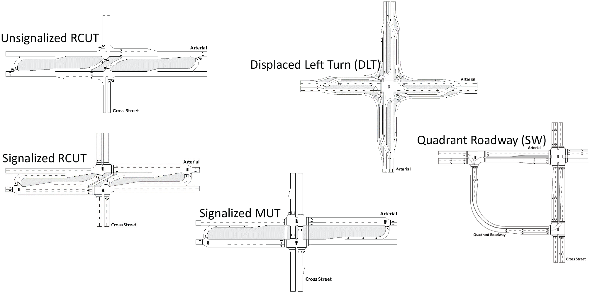
Sampling of common alternative intersection forms.

As the next section details, this research addresses coverage gaps that have motivated the development of a planning-level method for the “simultaneous” analysis of multiple AIIs, along with conventional intersection forms within the same computational platform that are best suited for ICE Stage II analysis ( 9 ). That platform is designed to accommodate both existing and potential new intersection forms in the future.

The paper is organized as follows. Subsequent to this introduction section, the paper presents a brief review of current practice for mobility analysis of intersection forms. This section is followed by a detailed description of the methodology including its general architecture, global and intersection-specific inputs, intermediate computations, and reported performance measures. A comparison of the method’s summary output against widely used analytical software is presented next. The paper concludes with some general findings and recommendations for future work.

Review of Current Practice

This review focuses on ICE Stage II tools for mobility analyses. A good starting point is the latest release of the Highway Capacity Manual (HCM7) (11). That release contains highly detailed operational analysis procedures for the evaluation of a limited set of AIIs. Facilities that are included in both HCM7 and its accompanying software tool (HCS8) include RCUTs under three types of control (merge/diverge, signalized, and yield controlled), MUTs under signalized and yield control, DDIs under both signal and yield control, and partial DLT under signal control. This is in addition to analysis procedures for both single and multilane roundabouts and conventional signalized and stop-controlled intersections.

At the planning level, NCHRP Report 825, Planning and Preliminary Engineering Applications Guide to the Highway Capacity Manual (PPEAG) ( 15 ), documents simplified procedures for conventional signalized and unsignalized intersections, some of which have been documented in Volume 4 of HCM7. That material includes computational spreadsheets for the analysis of signalized, two-way stop-controlled and single-lane roundabouts. The PPEAG, published in 2016, has no coverage of AIIs, a significant gap that this work addresses to enable the implementation of Stage II mobility assessment in ICE.

Synchro is another tool that is commonly used by practitioners for intersection operational analysis. It can also be utilized for the assessment of various AIIs during Stage II. Although Synchro is not as robust an evaluation tool as microsimulation software, it does enable a detailed assessment of the intersection operation, and provide the necessary outputs required during Stage II of an ICE process. However, Synchro has two major drawbacks during the analysis of AIIs. First, delays obtained from Synchro are at the intersection level and require additional, manual postprocessing of the outputs to derive the performance of AIIs to incorporate movement-based delays (based on origins and destinations) and to include the additional travel time experienced by drivers associated with an AII. In addition, certain intersection forms require complex signal phasing and lane configuration, making it difficult to accurately model in Synchro.

In summary, this review highlights the need to (a) develop comprehensive planning-level analysis procedures for a much larger set of AIIs than the current planning and operational methods do and (b) demonstrates the general accuracy of the proposed method against traditional operational method results.

Methodology

The proposed approach for developing planning-level AII procedures began by setting six guiding principles that were followed in the development process. Those are summarized below.

i. The method should not require an excessive number of inputs to implement. The use of default values for many parameters is highly desirable.

ii. The method should follow the approach used in the PPEAG signalized intersection method with a focus on movement group flow rate adjustments rather than adjustments to the saturation flow rates.

iii. The method should be implemented in an open-source platform, enabling access to the widest range of ICE practitioners.

iv. The method should enable simultaneous analyses of multiple intersection forms in a single run of the tool, consistent with the demand of Stage II ICE screening and similar in concept to FHWA’s CAP-X model.

v. The method should enable expandability of the tool to new and innovative intersection forms without disrupting the existing tool features.

vi. The method should produce performance measures that are sufficiently close to those generated by the more detailed operational methods, to engender confidence in its use by practitioners.

In the remainder of this paper, this new method will be referred to as “PPEAG-ICE”.

Scope of Coverage

The proposed method currently covers the analysis of 18 conventional and AII forms. About one-half of those can be analyzed either with the HCM7 (operational application) or in the PPEAG (planning application). Methods for the other half were developed under the auspices of NCHRP Project 17-98: Guide for Intersection Control Evaluation, and are included in the expanded spreadsheet tool, PPEAG-ICE. Table 1 summarizes the forms covered along with some of their properties and types of control. At this stage, unless otherwise noted, most of the intersection forms are signal controlled. The number of signal phases varies depending on the intersection location and type of control. The authors advise the readers to consult the informational guides referenced earlier for the operational details of the AIIs in Table 1.

Table 1.

Scope of Intersection Forms Included in HCM7, PPEAG, and PPEAG-ICE

Intersection form	Control type (S, U, B)	In HCM7 and/or PPEAG tool?	In new PPEAG-ICE tool?	In PPEAG-ICE
Intersection form	Control type (S, U, B)	In HCM7 and/or PPEAG tool?	In new PPEAG-ICE tool?	No. of intersections	Main intersection control	Remote intersection controls
Conventional signal	S	Y*	Y	1	S	NA
Two-way stop	US	Y*	Y	1	US	NA
All-way stop	US	Y**	Y	1	US	NA
Single-lane roundabout	UY	Y*	Y	1	UY	NA
Multilane roundabout	UY	Y	Y	1	UY	NA
Continuous green T	S	N	Y	1	S	NA
DDI	S	Y	Y	2	S (both)	NA
PDLT/PCFI	S	Y	Y	3	S	S
RCUT	S,U,B	Y (S,U,B)	Y(S)	4	S	S
MUT	S,U,B	Y (S,U,B)	Y(S)	3	S	S
PMUT	S,U,B	N	Y(S)	3	S	S
Quadrant road NE	S	N	Y	3	S	S
Quadrant road SE	S	N	Y	3	S	S
Quadrant road SW	S	N	Y	3	S	S
Quadrant road NW	S	N	Y	3	S	S
Bowtie intersection	S,UY	N	Y	4	S	UY
Forward jughandles	S,U	N	Y	5	S	S,U
Reverse jughandles	S,U	N	Y	5	S	S,U

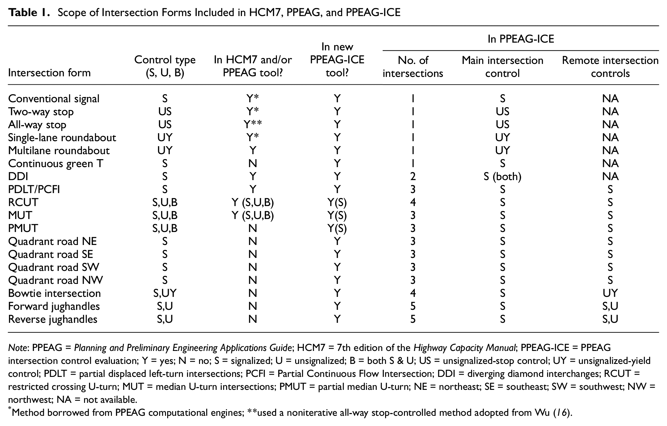
Note: PPEAG = Planning and Preliminary Engineering Applications Guide; HCM7 = 7th edition of the Highway Capacity Manual; PPEAG-ICE = PPEAG intersection control evaluation; Y = yes; N = no; S = signalized; U = unsignalized; B = both S & U; US = unsignalized-stop control; UY = unsignalized-yield control; PDLT = partial displaced left-turn intersections; PCFI = Partial Continuous Flow Intersection; DDI = diverging diamond interchanges; RCUT = restricted crossing U-turn; MUT = median U-turn intersections; PMUT = partial median U-turn; NE = northeast; SE = southeast; SW = southwest; NW = northwest; NA = not available.

Method borrowed from PPEAG computational engines; **used a noniterative all-way stop-controlled method adopted from Wu ( 16 ).

As indicated in Table 1, the PPEAG-ICE tool also includes a new, noniterative method for the analysis of single-lane all-way stop-controlled method (AWSC) intersections. This fills a void in the current PPEAG that has tools for conventional signals, two-way stop-controlled (TWSC) intersections but no AWSC tool. The added method, borrowed from a paper by Wu ( 16 ) is anchored around an average departure headway (t_B) and the volume of conflicting flows (Q_s). This includes movements departing from the same approach (entry conflicts), those that merge at the exit (exit conflicts), and those occurring in the intersection area proper (between conflicts). Figure 2 illustrates the movement conflicts for a conventional four-legged intersection under AWSC. Labels 1 to 4 pertain to exit conflict areas, whereas in-between conflict areas are labeled 5 to 8, and entry-level conflict areas are labeled 9 to 12. The figure is oriented to highlight those movements pertaining to the southmost approach (labeled “s” for subject approach). Here, r, o, and l specify the position of other approaches on the right (r), opposing (o), and left (l) of the subject one; L, T, R represent the left-, through, and right-turn movements, respectively, on those approaches; and F represents a conflict with crossing pedestrians. The idea is that during an hour the capacity of a movement is the difference between 1 h of departure time available and the time taken by its conflicting movement to discharge. In addition, a minimum capacity exists based on a fixed departure headway. The method does not account for pedestrians as conflicting movements. It is important to note that the overall intersection capacity is not taken as the sum of the individual lane capacities. This is because each approach-/lane capacity computation assumes that the conflicting flows stay at their current volumes. Thus, a sensible way to report an overall intersection capacity is to take the lowest combination of each lane- or approach capacity in combination with the prevailing flow rates on the other lanes. This will enable the analyst to determine the lowest feasible capacity at the intersection level.

Figure 2.

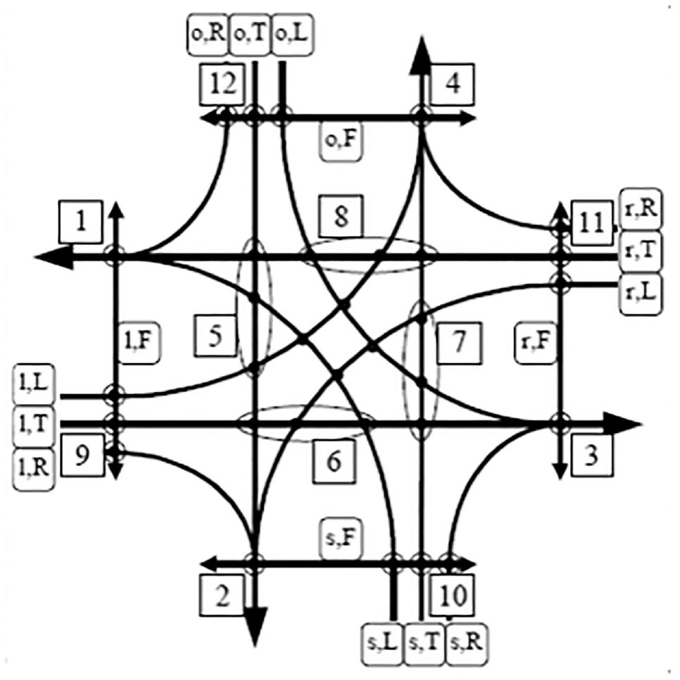
Designation of approach and conflicting movements at AWSC.

Tool Structure

The PPEAG-ICE tool is structured in a manner that satisfies the six guiding principles stated earlier. Regardless of the intersection form included, all model inputs and outputs follow the six basic blocks or modules depicted in Figure 3a . In the implementation spreadsheet of the method, each intersection form is given a separate tab, enabling the expansion of the current 18 intersection forms to additional tabs in the future. This pattern follows the general structure currently implemented in FHWA CAP-X. A brief explanation of each of the six module follows.

Figure 3.

(a) Method framework and (b) RCUT movement direction labeling scheme.

Global inputs: This module accepts inputs that are common to all intersection forms (see Figure 4). This includes the (typically) 12 turning movement flow rates, vehicle arrival type, peak hour factor, heavy vehicles’ percentage, major road free flow speed, distances between the main and remote intersections (when applicable), turn bay lengths for left- or U-turn movements and median width (for U-turn movements). Signal information include the local feasible minimum and maximum cycle lengths, the base saturation flow rate per lane and whether the green times for movement groups are to be estimated by the tool or entered by the user. Using global values follows the principle of minimizing user inputs for each model form. Intersection-form-specific inputs include the lane configuration at each intersection.

Figure 4.

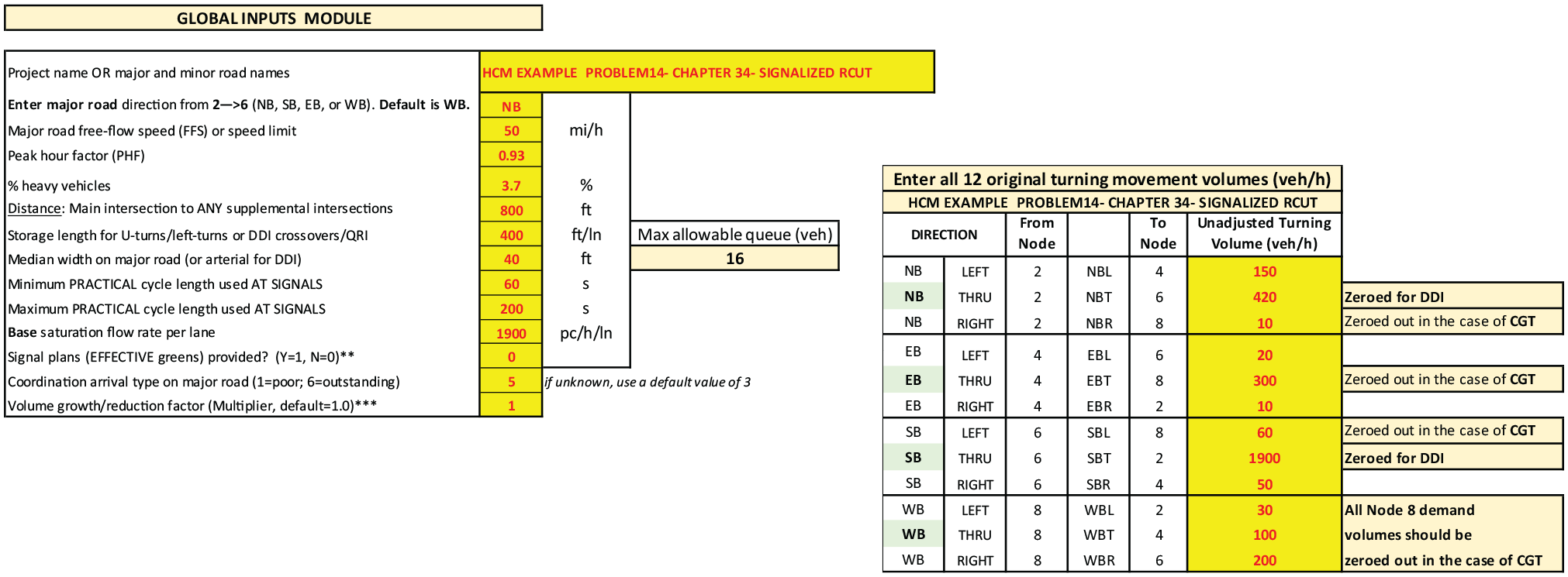
Screenshot of the global inputs module in the PPEAG tool.

An important global input concept is the designation of cardinal directions for all intersection movements. The tool assumes that the two approaches on the major road occur at Nodes 2 and 6, respectively. As a global input, the user must enter the cardinal direction (NB, EB, etc.) for the movement 2 → 6. The tool also assumes that the minor road approaches occur at Nodes 4 and 8. Finally, the tool assumes that Nodes 2–4–6–8 occur in a clockwise pattern. We illustrate this concept for an RCUT in Figure 3b . Here, the main road 2 → 6 cardinal direction was entered as westbound (WB). The user must enter that “WB” input value. The tool will automatically set the directional labels for all other movements. For example, movement 8 → 2 will be labeled southbound left (SBL) directly by the tool. In an efficient manner, the node numbers are also used to designate the four intersection positions, with 2 and 6 being the remote ones at an RCUT, and 4 and 8 the two main intersections. The only change in directional movement designation occurs for a DDI. There, Nodes 2 and 6 are on the freeway mainline whereas Nodes 4 and 8 represent movements on the main arterial road.

Movement performance measures: This module extracts the requisite demand volume inputs from the global inputs module, and converts them into passenger car equivalents in the peak period. Its other purpose is to convert movement group delays in the lane group (LG) module into individual movement delays. This process is highlighted by the upward right arrow in Figure 3a . Thus, in Figure 3b and in Table 2, the delay for the left-turning movement labeled 4 → 6 for the RCUT is the sum of three LG delays—highlighted in Table 2: the minor road right-turn LG delay at Intersection 4 + the U-turn LG delay at Intersection 2 + the major through LG delay at Intersection 8. Control delays for various movements are dependent on the signal phase(s) in which they move, the lane configurations at each intersection in their path and, in the case of left turns, on whether they operate in a protected or permissive phase.

Table 2.

Assigning Origin–Destination Movements to Intersection Turning Movements for RCUT

Intersection no.	Major left	Major throughs	Major rights	Minor rights	Minor U-turns
2	NA	24+26+28	NA	NA	48+46
4	24	62+82	64+84	42+48+46	NA
6	NA	68+62+64	NA	NA	84+82
8	68	26+46	28+48	82+84+86	NA

Note: RCUT = restricted crossing U-turn; NA = not available.

“4→6” represents the left turns from a minor road at an RCUT. This movement contributes to three turning movement group volumes at Intersections 2 (U), 4 (right), and 8 (through).

Since the 4 → 6 left-turn movement in Figure 3b is redirected, the additional extra distance travel time, twice the distance from Node 4 to 2 traversed at the free flow speed is added to generate the LOS measure, which is the overall experienced travel time by that movement. In addition, the tool reports an overall average system delay per Equation 1,

Average system delay = \sum_{i = 1}^{12} V_{i} d_{i} / \sum_{i = 1}^{12} V_{i}

(1)

where V_i and d_i are volumes and corresponding control delays for each of the 12 turning movements.

Intersection module: This module requires the user to enter the lane configuration (i.e., number of lanes, exclusive versus shared) for each intersection in the overall AII facility. That configuration will define the movement groups at each intersection. With this input, the tool will then assign the various origin–destination movements to turning movements at each intersection. Table 2 shows the assignment of the 12 origin–destination movement volumes to the four intersection turning movements for the RCUT facility in Figure 3b . Of note in Table 2 is the bold-labeled movement 46, representing the left turns from a minor road at an RCUT. This movement contributes to three turning movement group volumes at Intersections 2 (U), 4 (right) and 8 (through). Next, each group volume is converted to an equivalent through passenger car (TPC) units through a series of adjustment factors to account for turning movement maneuvers, lane utilization, and other nonideal conditions. This conversion is consistent with guiding principle (ii) discussed earlier. Finally, the adjusted TPCs are converted into LG flow ratios (v/s), and the critical flow ratios identified. In essence, this module develops the demand profile for each intersection LG, before determining the phasing and timing scheme.

Traffic control planning: As shown in Table 1, the tool assumes signalized control at all AII intersections. The exceptions to the rule are at bowtie intersections with yield controls at the minor road roundabouts, and at the termini of forward and reverse jughandle intersections with stop and/or yield control at each end. Given the demand volume input from the previous module, the tool estimates a practical cycle length at each intersection on the facility using the formula in Equation 2. The reported cycle length is always bounded by the minimum and maximum cycles in the global inputs module.

C = \frac{5 n \times 0.85}{0.85 - SCLV / S}

(2)

where

5n = total lost time per cycle, assuming 5 s/phase lost time and “n” critical phases (typically 2 or 3 at each AII signal);

0.85 = target volume-to-capacity (v/c) ratio for the critical movements; and

SCLV/S = sum of critical lane volumes divided by the adjusted saturation flow rate.

It is important to note that the PPEAG-ICE tool, although possibly proposing different practical cycle lengths for each intersection, still requires the user to manually enter the final cycle length at each signal. This is because a common (or ½ cycle) system cycle length across the arterial could be preferable to promote signal progression for through traffic on the main road. The user can either manually enter LG green times or have the tool calculate those, as specified in the global inputs module. In the latter case, green times are assigned to produce equal v/c ratios among all the critical LGs. For unsignalized controlled movements, the stop or yield capacity (c) is calculated from the conflicting traffic volume and default gap acceptance parameters. Those parameters will vary by movement, type of control, and maneuver difficulty. Equation 3 illustrates a typical unsignalized (TWSC, AWSC) capacity model used in the tool,

c = v_{c} \times \frac{\exp (- \frac{v_{c} T_{c}}{3600})}{1 - \exp (\frac{- v_{c} T_{f}}{3600})}

(3)

where

c = unsignalized (stop or yield) movement capacity in pc/h,

$v_{c}$ = conflicting flow rate in pc/h,

Tc = applicable critical headway (s), and

T_f = applicable follow up headway (s).

LG and intersection performance: This module uses the outputs from the previous two modules to calculate the v/c ratio, control delay and 95^th percentile queue for each LG at each intersection. Equations 4 to 7 depict the delay (d) and 95^th percentile queue (Q₉₅) models for signalized LGs,

d = d_{1} P F + d_{2}

(4)

d_{1} = \frac{0.50 C {(1 - \frac{g}{C})}^{2}}{{1 - \frac{g}{C} Min (1, X)}}

(5)

d_{2} = 225 [X - 1 + \sqrt[2]{{(X - 1)}^{2} + \frac{16 \times X}{c}}]

(6)

Q_{95} = \frac{2 \times 25 \times d \times c}{(3600 \times N)}

(7)

where

PF = progression factor. In the event an arrival type is specified for major road traffic, PF is computed based on the input arrival type platoon ratio (R_p ) and the green to cycle ratio (g/C). In the absence of such information, a default PF = 0.70 may be applied for well-progressed movements; PF = 1.25 for poorly progressed movements and PF = 1.0 for random arrivals;

$g =$ effective green time for the LG (s);

C = cycle length (s);

c = LG capacity in pc/h;

X = LG volume-to-capacity ratio; and

N = number of lanes in the LG.

The queue length model shown in Equation 7 is a simplified version that was borrowed from the current PPEAG. It assumes the 95^th percentile queue to be approximately twice the size of the average cycle queue. It is multiplied by 25 ft, which is the average spacing between vehicles at stop (jam spacing). The queue length value in feet is compared with the available queueing space for those movements operating in turn bays. In the case of unsignalized LGs, Equation 8 gives the expected control delay for those movements. Equation 7 is again used for the queue length estimation.

d = \frac{3, 600}{c} + 225 [X - 1 + \sqrt{{(X - 1)}^{2} + 32 \frac{X}{c}]}

(8)

Summary output: This module simply extracts the overall facility control delay (in Equation 1) from each AII tab in the tool, and provides a side-by-side comparison for screening purposes in Stage II ICE. A reproduction of this summary is depicted in Figure 5. The summary also reports whether any LG at any selected intersection is operating above its capacity. The user can then consult the appropriate tab to review and possibly remedy the problem LG.

Figure 5.

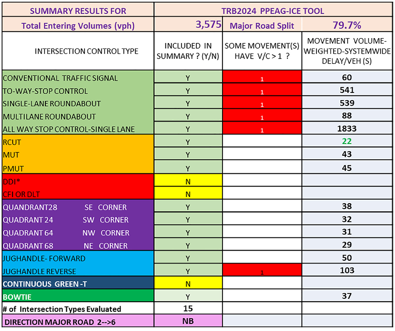
Screenshot of summary output module depicting system delay and outlier v/c ratios.

This module offers capabilities that are unavailable in any other ICE Stage II tool whether one uses analytical models or microscopic simulation. The comparison shown here ensures that (a) all inputs are identical that flow through the various intersection forms, (b) that the parameters’ default values are identical across the board, and (c) that all performance measures are movement rather than LG-based. Therefore, the comparison across intersection forms is truly objective and unbiased, even with the approximations made in various steps for a planning application level.

Tool Assessment

To evaluate the accuracy of the tool, the proposed PPEAG-ICE method system delays were compared with Synchro output and HCM7 example problem outputs for various intersection forms and under varying congestion levels. For the tool assessment and comparison, three types of intersections were used: (1) real-world case studies with actual traffic volumes, (2) NCHRP 17-98 “dummy” intersections with “made-up” volumes (but that are reasonable for the applications of AIIs such as intersections with high turn volumes), and (3) three example AII problems documented in HCM7. Table 3 and Figure 6 provide a comparison of system delay for those intersections using the results from the PPEAG-ICE method and from Synchro and HCM7. Overall delay was computed as the weighted average delay by movement volume (see Equation 1). Note that for Synchro results, individual intersection delay results must be postprocessed to calculate a system-level movement delay for each intersection form. The analysis results indicated that, overall, the PPEAG-ICE method produced very similar delay values compared with Synchro and HCM7. The difference in system delay between the PPEAG-ICE and the other platforms was within 5 s at almost all intersections, and in most cases less than 3 s, regardless of the level of congestion or intersection form tested. In fact, all 17 cases yielded identical LOS ratings for both methods.

Table 3.

Comparison of PPEAG-ICE, Synchro and HCM7 System Delays

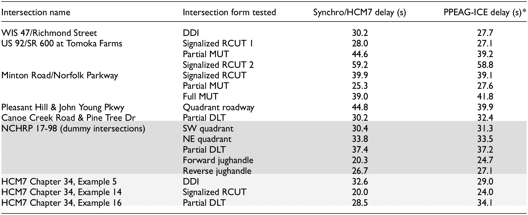
Note: PPEAG = Planning and Preliminary Engineering Applications Guide; HCM7 = 7th edition of the Highway Capacity Manual; PPEAG-ICE = PPEAG intersection control evaluation; DLT = displaced left-turn intersections; DDI = diverging diamond interchanges; RCUT = restricted crossing U-turn; MUT = median U-turn intersections.

For this case study, volumes scaled up to test a scenario in which volume-to-capacity (v/c) ratio is closer to 1.0 at the critical intersection.

Figure 6.

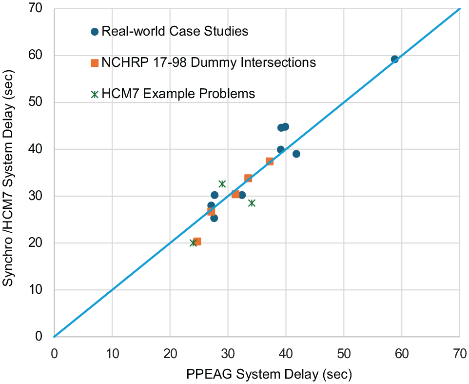
System delay data points layout: Synchro/HCM7 versus PPEAG-ICE.

A correlation analysis between the system delays estimated by the two methods yielded a correlation factor of r = 0.95 and a two-sample t-test could not reject the null hypothesis that the two delay distributions came from the same population. Some of the differences in delay were derived from several factors. The first was a result of differences in the value of the progression factor, since the default progression factor values tend to be somewhat conservative compared with typical progression factors with AIIs. The second was the differences in lost time as some of the real-world intersections have long change and clearance intervals (e.g., 4.5 s of yellow and 3.0 s of red clearance), which resulted in more than 5 s lost time for that phase (compared with the 5 s of lost time assumed in the PPEAG-ICE). Finally, in the case of the partial DLT (at the bottom of Table 2), the difference was from the use of a complex phasing scheme in HCM7, compared with the simple dual left phasing assumed in the PPEAG-ICE tool.

Summary and Conclusions

This paper summarizes the mobility component of NCHRP 17-98, which was aimed at providing detailed guidance for ICE. The focus of this component was to develop a new planning application and computational tools for the Stage II mobility analysis that could fill the current gap in coverage of the diverse (and expanding) suite of AIIs.

The design of the new proposed tool prioritized the simultaneous analysis of multiple AIIs within the same platform using a common input dataset. This feature of the tool guaranteed that alternative forms could be compared side-by-side under the same set of inputs and parameter assumptions using overall system delay as the key performance measure. In addition, the research developed a framework and a movement definition scheme that enables the extension of the current platform to accommodate new and yet to be conceived innovative intersection forms.

A comparison against a widely used commercial analytical platform yielded virtually identical system delays and identical LOS ratings across 17 case studies covering eight different AII forms and under varying intersection congestion levels. The maximum system delay difference between the two methods was about 5 s, with an average absolute difference of less than 2.5 s.

Importantly, the PPEAG-ICE tool required significantly less time to process and analyze various intersection forms in ICE. This was because of the following factors. First, common inputs are entered just once for all selected forms, rather than entering each time for each intersection form. Second, the tool does not require the user to develop new intersection models for each form, since each AII tab in the tool contains all intersections prepositioned in the right format. Finally, the tool automatically reports the overall system delay (at the movement level), an additional step that must be performed manually with other and alternative macroscopic tools.

Future plans for enhancing the tool will extend the scope of the current set with the addition of unsignalized AII forms, adding T-intersection designs, and including emerging AII forms ( 17 – 20 ).

Footnotes

Author Contributions

The authors confirm contribution to the paper as follows: study conception and design: B. Schroeder, N. Rouphail, data collection: B. Cesme; analysis and interpretation of results: N. Rouphail, B. Cesme; draft manuscript preparation: N. Rouphail, B. Cesme, B. Schroeder. All authors reviewed the results and approved the final version of the manuscript.

Declaration of Conflicting Interests

The authors declared the following potential conflicts of interest with respect to the research, authorship, and/or publication of this article: Nagui Rouphail, Burak Cesme, and Bastian Schroeder are employed by Kittelson and Associates, which has received funding for work on the Guide for Intersection Control Evaluation from TRB and from NCHRP. NCHRP is administered by TRB.

Funding

The authors disclosed receipt of the following financial support for the research, authorship, and/or publication of this article: This research is part of NCHRP Project 17-98, which is part of NCHRP. NCHRP is administered by TRB and funded by participating member states of the American Association of State Highway and Transportation Officials. NCHRP also receives critical technical support from FHWA, U.S. Department of Transportation.

ORCID iDs

Nagui M. Rouphail

Burak Cesme

Bastian Schroeder

References

FHWA. Restricted Crossing U-Turns: Informational Report. Report No. FHWA-SA-14-070. U.S. Department of Transportation, Washington, D.C., 2004.

FHWA. Diverging Diamond Interchange: Informational Guide. Report No. FHWA-SA-14-067. U.S. Department of Transportation, Washington, D.C., 2004.

NCHRP Research Report 959. Diverging Diamond Interchange Informational Guide, 2nd edition, Transportation Research Board, NAS, Washington, D.C., 2021.

FHWA. Median U-Turn Intersection: Informational Guide. Report No. FHWA-SA-14-069. U.S. Department of Transportation, Washington, D.C., 2014.

FHWA. Displaced Left Turn Intersection: Informational Guide. Report No. FHWA-SA-14-068. U.S. Department of Transportation, Washington, D.C., 2014.

FHWA. Quadrant Roadway Intersection: Informational Guide. Report No. FHWA-SA-19-029. U.S. Department of Transportation, Washington, D.C., 2020.

FHWA. Roundabouts: An Informational Guide. Report No. FHWA-RD-00-067. U.S. Department of Transportation, Washington, D.C., 2000.

NCHRP Research Report 1043. Guide for Roundabouts. Transportation Research Board, NAS, Washington, D.C., 2023.

NCHRP Research Report 1087. Guide for Intersection Control Evaluation. Transportation Research Board, NAS, Washington, D.C.

10.

FHWA. Capacity Analysis for Planning of Junctions, CAP-X. Report No. FHWA-SA-18-067. U.S. Department of Transportation, Washington, D.C., 2018.

11.

Highway Capacity Manual 7th Edition, A Guide for Multimodal Mobility Analysis. Transportation Research Board, NAS, Washington, D.C., 2022.

12.

SYNCHRO Studio 12. https://www.cubic.com/transportation/synchro-studio. Accessed June 25, 2023.

13.

PTV VISTRO. https://us-resources.ptvgroup.com/en-us/ptv-vistro. Accessed June 25, 2023.

14.

SIDRA Intersection 9.1. https://www.sidrasolutions.com/software/sidra-intersection. Accessed June 25, 2023.

15.

NCHRP Report 825. Planning and Preliminary Engineering Applications Guide to the Highway Capacity Manual (PPEAG). Transportation Research Board, NAS, Washington, D.C., 2016.

16.

Determination of Capacity at All-Way Stop-Controlled (AWSC) Intersections. Transportation Research Record: Journal of the Transportation Research Board, 2000. 1710: 205–214.

17.

Al-Omari

Abdel-Aty

Evaluation of New Intersection Designs, “Shifting Movements”. Transportation Research Record: Journal of the Transportation Research Board, 2021. 2675: 1352–1363.

18.

Shin

E. K.

Lee

J. H.

Kim

J. H.

Kim

J. S.

Jeong

Y. W.

Two Level Signalized Intersection. Transportation Research Record: Journal of the Transportation Research Board, 2008. 2060: 53–64.

19.

Mozdbar

Flipped Left Diamond Interchange. ITE Journal, Vol. 90, 2020, pp. 44–49.

20.

Zhao

An Alternative Design for the Intersections WithLimited Traffic Lanes and Queuing Space. IEEE Transactions on Intelligent Transportation Systems, Vol. 22, No. 3, 2021, pp. 1473–1483.