Comparative Analysis of Three Modeling Approaches for Predicting Pavement Conditions

Abstract

States, counties, and municipalities rely on pavement performance models to forecast future pavement conditions in their jurisdictions. Accurate prediction is essential for budget planning and the identification of candidates for rehabilitation. This study compares the performance of three different approaches to predict pavement conditions: (1) a sigmoidal or S-shaped curve; (2) a grey system model (GM); and (3) Gaussian process regression (GPR). All three models are trained on the same dataset for two types of pavements, asphalt with and without overlay and composite (i.e., asphalt over concrete), with each having two types of maintenance activities frequently performed by the South Carolina Department of Transportation. The trained models are then applied to separate test datasets. The prediction results indicate that GPR is the best model in three out of four cases using mean absolute error as the performance metric; the exception is the case involving the prediction of pavement serviceability index for asphalt pavement with mill-and-replace 1–2 in. + overlay 400 pounds per square yard rehabilitation treatment. When using mean absolute percentage error and root mean squared error as the performance metrics, the GPR model is the better model for predicting conditions of composite pavements, while the $GM (1, 1)$ model is the better model for predicting conditions of asphalt pavements.

Keywords

infrastructure infrastructure management and system preservation pavement management systems performance modeling

An integral element of a pavement preservation program for any state highway agency, county, or municipality is the ability to predict future conditions of pavements. Pavement performance models are developed for this purpose. In addition to being used to identify sections of roadways that need to be rehabilitated, they are also used to estimate and rationally allocate budget at the network level ( 1 ), evaluate the effectiveness of various rehabilitation treatments, and perform cost and benefit analyses ( 2 ). For these reasons, it is essential that pavement performance models yield accurate predictions of pavement conditions.

Most state agencies use some form of regression model, and some agencies use the S-shaped model, to predict pavement conditions because of their simplicity in model estimation and application ( 3 , 4 ). Both S-shaped models and multiple linear regression models are considered deterministic models. According to Montenegro ( 5 ), as a rule of thumb, a sample size of at least 10 times the number of parameters is needed when the ordinary least squares method is used to estimate the parameters. Thus, if a model has three parameters, the sample size should be at least 30. This sample size requirement is problematic for smaller agencies that do not have the resources to collect pavement condition data frequently. Additionally, there are situations in which the sample size may be limited, such as using project-level pavement condition data to determine the optimal maintenance plan to prolong the life of the pavement.

To overcome the problem of limited sample size, some researchers have explored the use of grey models (GMs) that are based on grey system theory. A GM is a system model based on an ordinary differential equation (ODE) in which some of the model parameters are unknown. GMs are often identified by two parameters, $i$ and $j$ as in $GM (i, j)$ where $i$ is the order of the ODE and is the number of variables. In a GM, the unknown function in the ODE is not constructed; instead, it is replaced by a surrogate model constructed from observed data. GMs have been applied widely and proven to be useful in solving uncertain problems with small sample sizes. However, their application in the area of pavement condition prediction is quite limited. The lone study found applied a $GM (1, 1)$ to predict pavement deterioration after receiving a micro-surfacing treatment ( 6 ). It remains unclear whether GMs are suitable for predicting pavement conditions for other pavement types and rehabilitation treatments. This study seeks to provide insight into this topic.

There is a growing body of literature exploring machine-learning techniques for pavement performance prediction. Computational methods available in the machine-learning field include artificial neural networks, support vector machines, Gaussian process regression (GPR), and recurrent neural networks, among others. Among the machine-learning techniques, GPR has been shown to work well in applications that have small sample sizes ( 7 – 9 ); it is a non-parametric, Bayesian approach to regression. Another strength of GPR is that it does not over-fit the data. To date, no machine-learning methods have been applied to predict pavement conditions using a small sample size. This study seeks to address this gap in the literature. The research questions are: (1) can GPR be used to predict pavement conditions using a relatively small number of observations, and (2) how well does it compare with GMs and deterministic models, particularly an S-shaped model?

The objective of this paper is to assess the performance of GM and GPR models compared with the commonly used S-shaped models to predict pavement conditions using a relatively small sample size. The assessment is performed using South Carolina pavement functional and structural condition data. For the model training and testing, two types of pavements and two types of rehabilitation methods are chosen. The two pavement types are asphalt and composite (i.e., asphalt over concrete). These two pavement types make up the majority of pavements on interstates in South Carolina. The two rehabilitation methods are mill-and-replace 2–4 in. + OL 200 PSY (200 pounds per square yard overlay) and mill-and-replace 1–2 in. + OL 400 PSY. These two rehabilitation methods are the most frequently used treatments in the last 10 years in South Carolina by the number of projects and total lane miles. Once the models are trained, they are evaluated on a separate test dataset using the root mean square error (RMSE), mean absolute percentage error (MAPE), and mean absolute error (MAE) performance measures.

The remainder of this paper is organized as follows. The next section provides a review of relevant studies. The third section presents the methodology and data used in this study. The fourth section presents and discusses the results. Finally, the fifth section provides a summary of the study and concluding remarks.

Literature Review

Many studies have developed methods to predict pavement conditions accurately. The following review is limited to those that used deterministic, GM, and GPR models.

Deterministic Models

Shahin et al. ( 10 ) evaluated three mathematical curve-fitting techniques for modeling pavement condition index. The model they found to work best is a polynomial function where $x$ is the age of the treated pavement. Abaza ( 11 ) found simple regression models with the age of the treated pavement as the sole independent variable to have the best performance. Prozzi and Hong ( 12 ) found exponential regression to provide the best agreement. Instead of using only the age of the treated pavement as the variable, Rahman et al. ( 13 ) considered other variables, including annual average daily traffic, free flow speed, precipitation, temperature, and soil type. Luo and Chou ( 14 ) found that clusterwise linear regression outperformed the traditional regression method.

State departments of transportation (DOTs) have sponsored several research projects to develop or improve on their existing pavement deterioration models. George et al. ( 15 ) developed an exponential regression model for the Mississippi DOT. Chan et al. ( 16 ) also found exponential regression to model pavement condition rating well for North Carolina DOT. With the goal of using the least number of independent variables, Gulen et al. ( 17 ) developed a regression model for Indiana DOT with age and annual average daily traffic (AADT) as independent variables. Similarly, Kim and Kim ( 18 ) evaluated the performance of three different regression models, with one to three independent variables, for the Georgia DOT. The model with three variables has service year, AADT, and interaction of service year and AADT as independent variables. For Kentucky DOT, Xu et al. ( 19 ) developed a regression model that yielded comparable performance to an artificial neural network. Their regression model has the cracking index, pavement age, average daily traffic, and International Roughness Index (IRI) as the independent variables. Tsai et al. ( 20 ) found the S-shaped or sigmoidal function to provide a good fit in a study sponsored by Georgia DOT.

Grey Model

Yu et al. ( 6 ) proposed a new Pavement Quality Index (PQI) model, which is a weighted function of four factors: 1) pavement condition index, 2) riding quality index, 3) rut depth, and 4) skid resistance index. Because of the need to determine the appropriate weights for these four factors, the authors proposed the use of GM. The authors reasoned that GM is suitable for situations where the collected pavement data may not correlate perfectly with actual conditions. The authors concluded that a GM(1,1) provided reasonable results for predicting the PQI of pavements that received micro-surfacing treatments. Tang and Xiao ( 21 ) also used a GM(1,1) to predict PQI. They found that applying monthly attenuations (defined as the difference in PQI between successive years) not only effectively lowered the condition number of the matrix but also ensured that the relative error was small. Zhang et al. ( 22 ) developed separate GM(1,1) models to estimate pavement smoothness, rut, and skid resistance. They assessed their models’ performance against field-measured data and found them to yield excellent accuracy based on the residuals and grey absolute correlation. Unlike previous studies, Du and Shen ( 23 ) derived a multivariate GM for which the function contains the previously measured rut depth and the number of loading cycles representing the traffic loading. Since there are two variables, their GM is a GM(1,2). Their analysis showed that 95 of the 96 rutting predictions were within the 2.5 mm tolerance level.

Gaussian Process Regression

The only study that has applied GPR to predict road surface conditions is the work of Heyns et al. ( 24 ). The authors proposed a speed calibration methodology, in which the underlying condition of the road is considered during the calibration phase. This approach makes it possible to obtain a dynamic calibration function that adjusts itself to the instantaneous nature of the road that the vehicle traverses. The dynamic calibration function was implemented by GPR. The results indicated that the proposed methodology may potentially be of use as a generic, simple, and cost-effective approach to perform real-time road condition monitoring.

Literature Review Summary

From the above review, it can be concluded that prior work using GM or GPR to predict pavement conditions is inconclusive in regard to their performance against commonly used deterministic methods for different pavement types and treatment types. To address this shortcoming, this study is the first to assess the performance of a GM and a GPR model to predict the condition of asphalt and asphalt over concrete pavements for mill-and-replace rehabilitation methods. The aim is to gain insight into whether a semi-parametric model (GM) and a non-parametric model (GPR) outperform the traditional parametric model (S-shaped).

Methods

Data Description

The primary interest of this study is to model pavement deterioration over time after receiving a rehabilitation treatment. The pavement serviceability index (PSI), a measure of pavement rideability, and pavement distress index (PDI), a measure of pavement distress, were selected to represent the pavement functional and structural conditions for which we want to estimate ( 4 ). PSI and PDI are two indices used by the South Carolina DOT (SCDOT) to quantify PQI. PQI is an overall rating index with a theoretical scale from 0 to 5, where 5 is considered a perfectly plane and distress-free pavement. PSI is related to the IRI as shown in the following equation.

PSI = 5 \times e^{(- 0.004 \times IRI)}

(1)

Equation 1 yields a PSI value between 0 and 5, where 5 represents a perfectly smooth pavement surface. IRI is collected every one-tenth of a mile and is measured in inches per mile. For modeling purposes, an average PSI is used for the entire road section that was rehabilitated. Thus, each road section, regardless of its length, will have only one PSI value. For example, if a rehabilitation project involves a 1 mi long road section, then 10 IRI measurements are used to compute an average IRI per year, from which the average PSI is determined using Equation 1.

To calculate PDI, detailed distress data must be converted into a single scale index. For flexible (bituminous and composite) pavements, there are six recognized types of distresses: fatigue cracking, transverse cracking, longitudinal cracking, rut depth, patching, and raveling. For rigid (concrete) pavements, eight types of distresses are observed: surface deterioration, transverse cracking, longitudinal cracking, patching, punchouts, spalling, faulting, and pumping. The distress data are input as extent (percentage distressed area) and severity (low, moderate, high) for each observed distress location. The procedure SCDOT uses to calculate PDI is described in a report entitled South Carolina HPMA Index Models developed by Stantec ( 25 ). Similar to PSI, a PDI ranges from 0 to 5, where 5 represents a perfect (distress-free) pavement.

The PSI and PDI data used to train and test the performance of the models (S-shaped, GM, and GPR) in this study were provided by SCDOT. These data are shown in Tables 1 to 4. Each table contains data collected for a particular type of pavement that received a specific type of rehabilitation treatment. SCDOT has a different prediction model for each combination of pavement type and rehabilitation method. Each of the four datasets shown in Tables 1 to 4 is used to train and test the models ( 4 ). About 70% of the observations $(n = 345)$ were used for training and about 30% were used for testing $(n = 147)$ . Each observation is a project. Among the 492 projects, 147 were for mill-and-replace 2–4 in. + OL 200 PSY for asphalt pavement, 92 were for mill-and-replace 2–4 in. + OL 200 PSY for asphalt over concrete pavement, 106 were for mill-and-replace 1–2 in. + OL 400 PSY for asphalt pavement, and 147 were for mill-and-replace 1–2 in. + OL 400 PSY for asphalt over concrete pavement. Note that 200 PSY overlay is equivalent to 2 in. overlay and 400 PSY overlay is equivalent to 4 in. overlay.

Table 1.

Segments Containing PSI and PDI Data for Mill-and-Replace 2–4 in. + OL 200 PSY for Asphalt Pavement

Route	Number of years of data available	Date range	Length (miles)
I-185 N	10	2011–2020	2.57
I-26 W	8	2013–2020	8.73
I-77 N	8	2013–2020	16.741
I-20 W	9	2012–2020	6.5
I-85 N	10	2011–2020	1.73
I-26 W	9	2012–2020	16.88
I-26 W	10	2011–2020	4.85
I-77 N	10	2011–2020	3.57
I-85 S	10	2011–2020	6.73
I-85 S	10	2011–2020	2.6
Total			70.90

Note: PSI = pavement serviceability index; PDI = pavement distress index; OL 200 PSY = 200 pounds per square yard overlay; N = north; W = west; S = south.

Table 2.

Segments Containing PSI and PDI Data for Mill-and-Replace 2–4 in. + OL 200 PSY for Asphalt over Concrete Pavement

Route	Number of years of data available	Date range	Length (miles)
I-26 E	10	2011–2020	5.1
I-26 E	10	2011–2020	8.68
I-85 N	9	2012–2020	3.99
I-26 W	9	2012–2020	5.72
I-77 S	10	2011–2020	3.99
I-526 E	8	2013–2020	2.02
I-20 W	4	2017–2020	14.16
I-95 S	4	2017–2020	15.33
I-85 S	10	2011–2020	7.92
I-385 S	7	2014–2020	4.37
Total			71.28

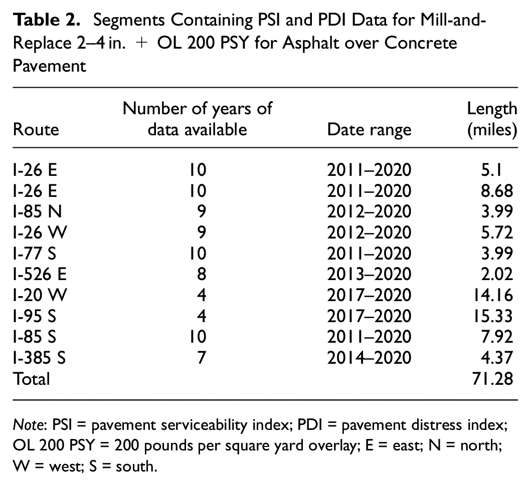
Note: PSI = pavement serviceability index; PDI = pavement distress index; OL 200 PSY = 200 pounds per square yard overlay; E = east; N = north; W = west; S = south.

Table 3.

Segments Containing PSI and PDI Data for Mill-and-Replace 1–2 in. + OL 400 PSY for Asphalt Pavement

Route	Number of years of data available	Date range	Length (miles)
I-20 E	6	2015–2020	21.3
I-20 E	6	2015–2020	21.3
I-20 W	7	2014–2020	6.36
I-20 W	7	2014–2020	10.6
I-20 W	8	2013–2020	5.81
I-26 E	10	2011–2020	9.25
I-26 E	9	2012–2020	4.55
I-77 S	8	2013–2020	15.94
I-85 N	10	2011–2020	7.38
I-20 E	9	2012–2020	5.78
Total			108.27

Note: PSI = pavement serviceability index; PDI = pavement distress index; OL 400 PSY = 400 pounds per square yard overlay; E = east; W = west; S = south; N = north.

Table 4.

Segments Containing PSI and PDI Data for Mill-and-Replace 1–2 in. + OL 400 PSY for Asphalt over Concrete Pavement

Route	Number of years of data available	Date range	Length (miles)
I-20 E	10	2011–2020	14.54
I-20 E	10	2011–2020	6.1
I-185 S	9	2012–2020	2.07
I-26 E	4	2017–2020	7.15
I-20 W	5	2016–2020	11.14
I-26 E	9	2012–2020	4.44
I-26 E	6	2015–2020	17.5
I-26 E	5	2016–2020	1.02
I-26 E	9	2012–2020	12.68
I-95 S	6	2015–2020	5.35
Total			81.99

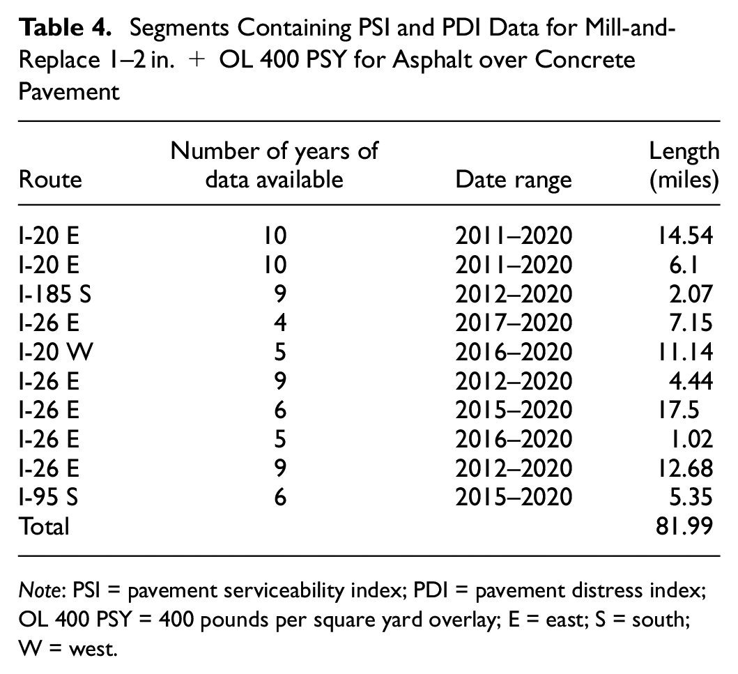
Note: PSI = pavement serviceability index; PDI = pavement distress index; OL 400 PSY = 400 pounds per square yard overlay; E = east; S = south; W = west.

Figures 1 and 2 show the average PSI and PDI of each segment over time for each treatment method and pavement type, respectively. Note that year 0 denotes the year the pavement segment was rehabilitated. It can be seen that the average PSI trends do not exhibit a monotonic decreasing trend. Taking Figure 2a (MR 2–4 in. + OL 200 PSY for asphalt pavement), for example, the PSI decreased slightly from year 7 to 8 and increased from year 8 to 9. Possible reasons include the use of different segments across the entire state and the use of different equipment and vendors to collect the IRI. Also, note that the PSI and PDI data exhibit serial correlation and are non-stationary.

Figure 1.

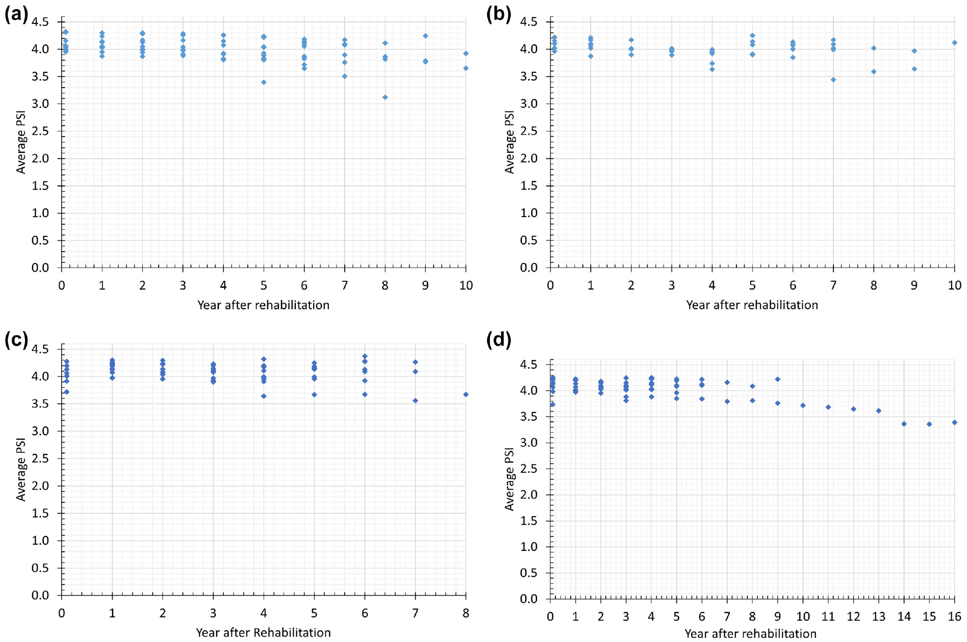
Average PSI of segments by treatment method and pavement type: (a) MR 2–4 in. + OL 200 PSY for asphalt pavement, (b) MR 2–4 in. + OL 200 PSY for asphalt over concrete pavement, (c) MR 1–2 in. + OL 400 PSY for asphalt pavement, and (d) MR 1–2 in. + OL 400 PSY for asphalt over concrete pavement.

Figure 2.

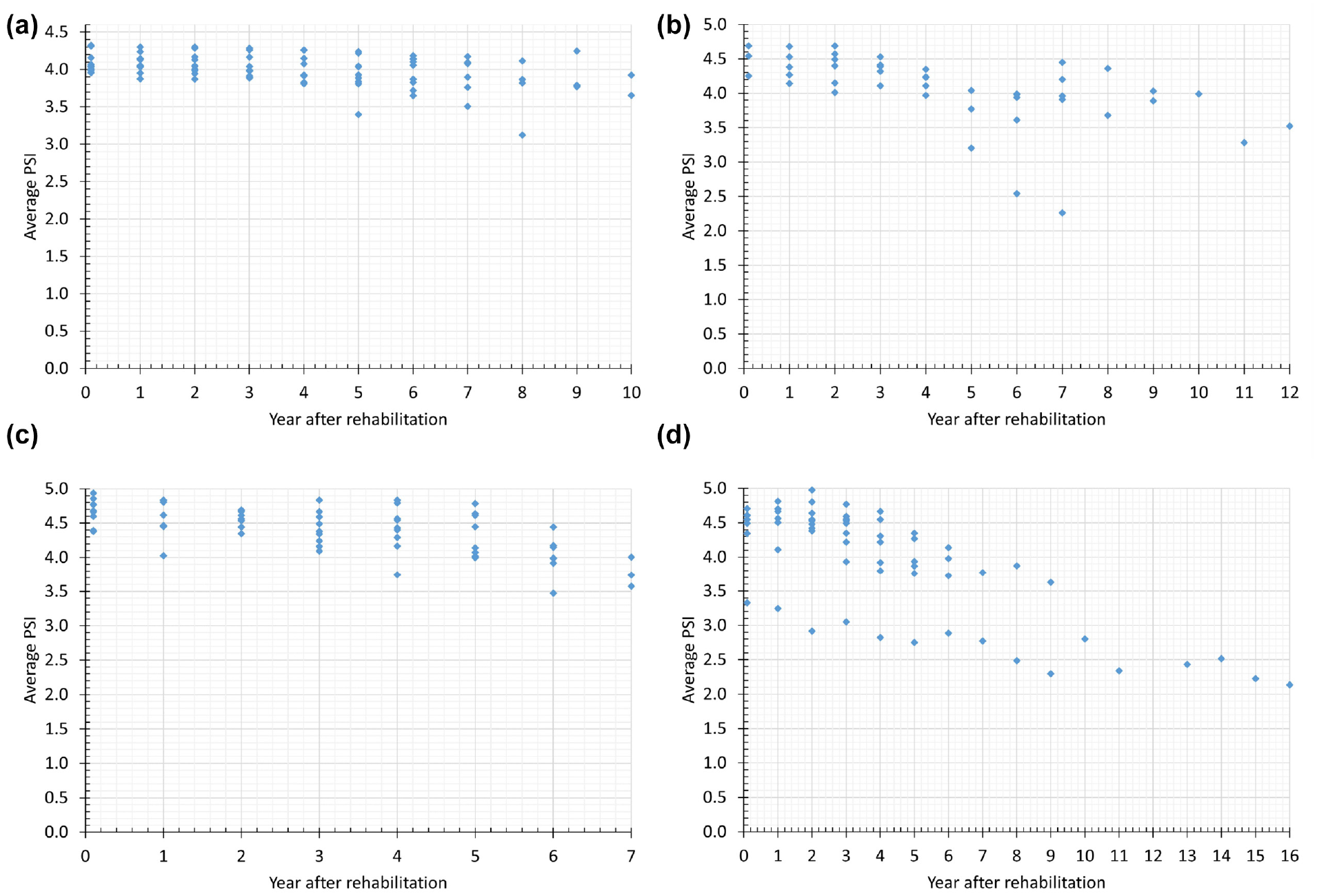
Average PDI of segments by treatment method and pavement type: (a) MR 2–4 in. + OL 200 PSY for asphalt pavement, (b) MR 2–4 in. + OL 200 PSY for asphalt over concrete pavement, (c) MR 1–2 in. + OL 400 PSY for asphalt pavement, and (d) MR 1–2 in. + OL 400 PSY for asphalt over concrete pavement.

Grey System Model—GM(1,1)

To model a time series, grey system theory ( 26 ) provides a family of GMs, where the most basic one is the first-order GM with one variable, often referred to as GM(1,1). The principles and estimation of GM(1,1) are briefly discussed here. Readers are referred to the work of Ju-Long ( 25 ) for additional information. Suppose that $X^{(0)} = (x^{(0)} (1), x^{(0)} (2), . . ., x^{(0)} (k))$ denotes a sequence of $k$ nonnegative observations of a stochastic process, and $X^{(1)} = (x^{(1)} (1), x^{(1)} (2), . . ., x^{(1)} (k))$ is an accumulation sequence of $X^{(0)}$ computed as:

x^{(1)} (k) = \sum_{i = 1}^{k} x^{(0)} (i)

(2)

The original form of GM(1,1) is defined by the following equation ( 4 ).

x^{(0)} (k) + a x^{(1)} (k) = b

(3)

Let $Z^{(1)} = (z^{(1)} (2), z^{(1)} (3), . . ., z^{(1)} (k))$ be a mean sequence of $X^{(1)}$ where

z^{(1)} (k) = \frac{z^{(1)} (k - 1) + z^{(1)} (k)}{2}, \forall k = 2, 3, \dots, n

(4)

The basic form of GM(1,1) is given by the following equation.

x^{(0)} (k) + a z^{(1)} (k) = b

(5)

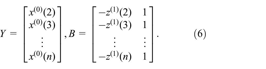
If $(\hat{a}, \hat{b})^{T} = (a, b)^{T}$ and

Y = [\begin{matrix} x^{(0)} (2) \\ x^{(0)} (3) \\ ⋮ \\ x^{(0)} (n) \end{matrix}], B = [\begin{matrix} - z^{(1)} (2) & 1 \\ - z^{(1)} (3) & 1 \\ ⋮ & ⋮ \\ - z^{(1)} (n) & 1 \end{matrix}] .

(6)

then, as in the work of Liu and Lin ( 27 ), the least squares estimate of the GM(1,1) model is $(\hat{a}, \hat{b})^{T} = (B^{T} B)^{- 1} B^{T} Y$ . Suppose that ${\hat{x}}^{(0)} (k)$ and ${\hat{x}}^{(1)} (k)$ represent the original time response sequence and the accumulated time response sequence of the GM at time $k$ , respectively, then the latter can be obtained by solving Equation 7 (whitenization equation of the GM(1,1) model). The solution to Equation 7 is shown in Equation 8.

\frac{d x^{(1)}}{dt} + a x^{(1)} (k) = b

(7)

{\hat{x}}^{(1)} (k + 1) = (x^{(0)} (1) - \frac{b}{a}) e^{- ak} + \frac{b}{a}, k = 1, 2, . . ., n

(8)

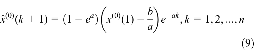
According to the definition in Equation 5, the restored values of ${\hat{x}}^{(0)} (k + 1)$ are calculated as ${\hat{x}}^{(1)} (k + 1) - {\hat{x}}^{(1)} (k)$ . Essentially, we are taking derivatives at step $k$ because we are calculating the slope for this interval. This step results in Equation 9.

{\hat{x}}^{(0)} (k + 1) = (1 - e^{a}) (x^{(0)} (1) - \frac{b}{a}) e^{- ak}, k = 1, 2, . . ., n

(9)

which can be used to produce forecasts for $x^{(0)} (k + 1), x^{(0)} (k + 2)$ , and so on.

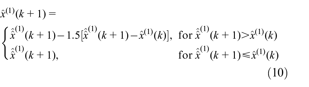
In this study, Equation 9 is the main forecasting equation that generates values $x^{(0)} (k + 1), x^{(0)} (k + 2)$ , $\forall k = 2, 3, . . ., n$ . The $GM (1, 1)$ model can be used to forecast one or more future data points: ${\hat{x}}^{(0)} (k + w + 1), {\hat{x}}^{(0)} (k + w + 2)$ , and so forth, using a fixed interval, $w$ , of prior pavement condition data: $x^{(0)} (k + 1), x^{(0)} (k + 2), . . ., x^{(0)} (k + w)$ , where $w \geq 4$ (e.g., $w = 4$ is found to produce very good results). Then the process is repeated where the fixed interval is shifted to the next period, and the model is used to calculate $x^{(0)} (k + 2), x^{(0)} (k + 3), . . ., x^{(0)} (k + n)$ , where $n$ denotes the desired future $n^{th}$ year for which data need to be estimated. Moreover, GM models are run as a rolling horizon framework. Using past $w = 4$ PSI observations, parameters $a, b$ are estimated (updated), and a prediction is generated for the $5^{th}$ PSI values. As expected in this framework, predictions can be higher than the previous PSI values. Thus, they are smoothed using a simple expression ${\hat{x}}^{(1)} (k + 1) = 0.50 min_{[0 : k]} {\hat{x}}^{(1)} (k) + 0.25 min_{[0 : k]} x_{k} + 0.25 {\bar{\hat{x}}}_{0 : k}$ . If current predicted PSI or PDI is higher than the previous PSI or PDI prediction, then, Equation 10 adjusts the prediction by incorporating a decreasing half of the previous one.

\begin{matrix} {\hat{x}}^{(1)} (k + 1) = \\ {\begin{matrix} {\hat{\hat{x}}}^{(1)} (k + 1) - 1.5 [{\hat{\hat{x}}}^{(1)} (k + 1) - {\hat{x}}^{(1)} (k)], & for {\hat{\hat{x}}}^{(1)} (k + 1) > {\hat{x}}^{(1)} (k) \\ {\hat{\hat{x}}}^{(1)} (k + 1), & for {\hat{\hat{x}}}^{(1)} (k + 1) \leq {\hat{x}}^{(1)} (k) \end{matrix} \end{matrix}

(10)

The number of conditions of the GM model matrix needs to be small to produce accurate estimates. A condition number for a matrix and related computational task measures how sensitive the answer is to perturbations in the input data and roundoff errors made during the solution process. The definition of the condition number depends on the choice of norm. When a matrix is said to be “ill-conditioned,” it refers to the sensitivity of its inverse, that is, of the condition number for inversion, and not of all the other condition numbers. If the condition number is not too much larger than one, the matrix is well-conditioned, which means that its inverse can be computed with good accuracy. If the condition number is very large, then the matrix is said to be ill-conditioned. Practically, such a matrix is almost singular, and the computation of its inverse, or solution of a linear system of equations, is prone to large numerical errors. If a matrix is not invertible, the condition number is taken to be infinity.

When applying the GMs to predict pavement condition using the South Carolina PSI and PDI data shown in Tables 1 to 4, its matrix was found to be ill-conditioned. This is because of having values that are similar or repeating in the input data. This general problem of the grey GM(1,1) model has been observed by Tang and Xiao ( 21 ). To overcome this issue, a Gaussian noise $~ N (0, 0.0001)$ was added to make values slightly different from each other to allow one of the multiple solutions to be found.

GPR Models

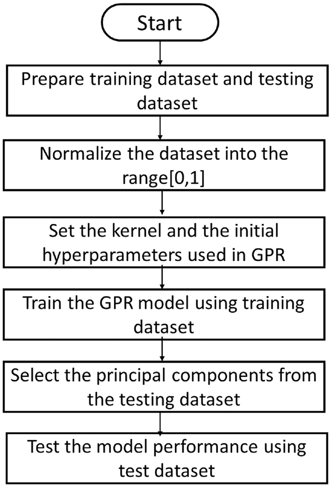
Figure 3 shows the steps followed in this study to train and test the GPR model. Following the methodology presented in Zeng et al. ( 28 ), the prediction function of a linear regression model is:

y_{*} = β_{0} X_{*} + β_{1} + ε_{t}

(11)

where $X_{*}$ is the matrix of input which is the age, and $y_{*}$ is the matrix of output which is PSI; $β_{0}$ and $β_{1}$ are coefficients to be estimated, and they contribute to the linear relationship between the inputs and outputs; and $ε_{t}$ is a noise term. GPR assumes that the $ε_{t}$ follows a Gaussian distribution with a mean of $0$ and a variance of $θ_{n}^{2}$ :

ε_{t} ~ N (0, θ_{n}^{2})

(12)

Figure 3.

GPR model development and testing procedure.

The marginal likelihood of the sample data can be expressed as follows:

p (y | X) ~ N (0, K_{N} + θ_{n}^{2} I)

(13)

where $K_{N}$ represents the covariance matrix for the training set, $I$ is the identity matrix, and $θ_{n}^{2}$ is the variance of the noise term. The noise terms are assumed to be identical, independently distributed (IID) random variables.

Given the observed outputs $y$ , the training input matrix $X$ , and the noise variance $θ_{n}^{2}$ , the predictive distribution of the unseen outputs $y_$ , conditioned on the new input matrix $X_$ , can be expressed as follows.

p (y_{*} | X_{*}, X, y) ~ N (μ_{*}, θ_{n}^{2} I)

(14)

μ_{*} = K_{* N} (K_{N} + θ_{n}^{2} I)^{- 1} y

(15)

θ_{*}^{2} = K_{* *} - K_{* N} (K_{N} + θ_{n}^{2} I)^{- 1} K_{N *}

(16)

In the above equations, $μ_{*}$ is the mean value of the Gaussian process posterior mean, $θ_{*}^{2}$ is the covariance matrices of prediction, $K_{* N}$ represents the covariance matrix between the training and testing datasets, $θ_{n}^{2}$ is the variance of the noise term, $X_{*}$ is the testing dataset, and $X$ is the training dataset.

The kernel, also known as the covariance function, plays a fundamental role in characterizing the covariance of the Gaussian process random variables. In conjunction with the mean function, the kernel serves as the defining component of a Gaussian process. An inherent problem with all kernels employed in GPR models (e.g., covLIN, covLINard, covMaterniso, covNoise, covPeriodic, covRQard, and covRQiso) is the adaptation to the trends observed in the training datasets, thereby producing predicted PSIs that could fluctuate from year to year, which would be incorrect. The pavement deterioration rate is expected to be monotonically decreasing. That is, the PSI of a pavement segment in a given year cannot be greater than the PSI from the previous year unless it was rehabilitated. To overcome the kerner’s inherent fluctuation characteristic, this study proposes to combine the following two kernels to yield the desired pavement deterioration behavior, thereby improving the model’s predictive power.

Radial-basis function (RBF) kernel:

k (x_{i}, x_{j}) = \exp (- \frac{d {(x_{i}, x_{j})}^{2}}{2 l^{2}})

(17)

where $d (x_{i}, x_{j})$ is the Euclidean distance and $l$ is the length-scale parameter which must be positive $(l > 0)$ .

Matern kernel:

k (x_{i}, x_{j}) = \frac{1}{Γ (ν {) 2}^{ν - 1}} (\frac{\sqrt{2 ν}}{l} d {(x_{i}, x_{j})}^{ν} K_{ν} (\frac{\sqrt{2 ν}}{l} d (x_{i}, x_{j}))

(18)

where $K_{ν} (\frac{\sqrt{2 ν}}{l} d (x_{i}, x_{j}))$ is the modified Bessel function, $Γ (ν)$ is the Gamma function, and $ν$ is a positive parameter that controls the smoothness of the kernel function. The value of $ν$ determines the degree of differentiability of the sample paths of the Gaussian process defined by the kernel.

Results and Discussion

To evaluate the performance of the GM(1,1) model and the GPR model, their predicted PSI and PDI for the test datasets were compared against the predicted values of the following S-shaped model ( 29 ):

y_{i} = \frac{a}{1 + \exp (- \frac{x_{i} - b}{c})}

(19)

where $y_{i}$ is the PSI to be predicted in the $i^{th}$ year, $x_{i}$ is the corresponding pavement age, and $a$ , $b$ , and $c$ are parameters of the model that need to be estimated based on observed data.

The metrics used to assess the performance of the models were: RMSE, MAE, and MAPE. According to Uwanuakwa et al. ( 30 ), evaluation of model performances should include RMSE and MAE at a minimum.

MAPE = (\frac{1}{N} \sum_{i = 1}^{i = N} (\frac{| PS I_{i, act} - PS I_{i, est} |}{PS I_{i, act}})) 100 %

(20)

where $N$ is number of observations, $PS I_{i, act}$ is observed PSI in year $i$ , and $PS I_{i, est}$ = estimated PSI in year $i$ .

RMSE = \sqrt{\frac{\sum_{i = 1}^{i = N} {(PS I_{i, act} - PS I_{i, est})}^{2}}{N}}

(21)

MAE = \frac{1}{N} \sum_{i = 1}^{i = N} | PS I_{i, act} - PS I_{i, est} |

(22)

As mentioned in the “Methods” section, a contribution of this study is the use of a smoothing function (i.e., Equation 10) with the GM(1,1) model to avoid having a predicted PSI or PDI higher than the previous value. The effect of smoothing can be observed in Figure 4a. Another contribution is the use of two kernels (i.e., radial basis and Matern) instead of just one (radial basis) for the GPR model. The effect of using two versus one kernel for the GPR model can be observed in Figure 4b. In the following, all reported results for the GM(1,1) model include the use of the smoothing function and all reported results for the GPR model are with two kernels.

Figure 4.

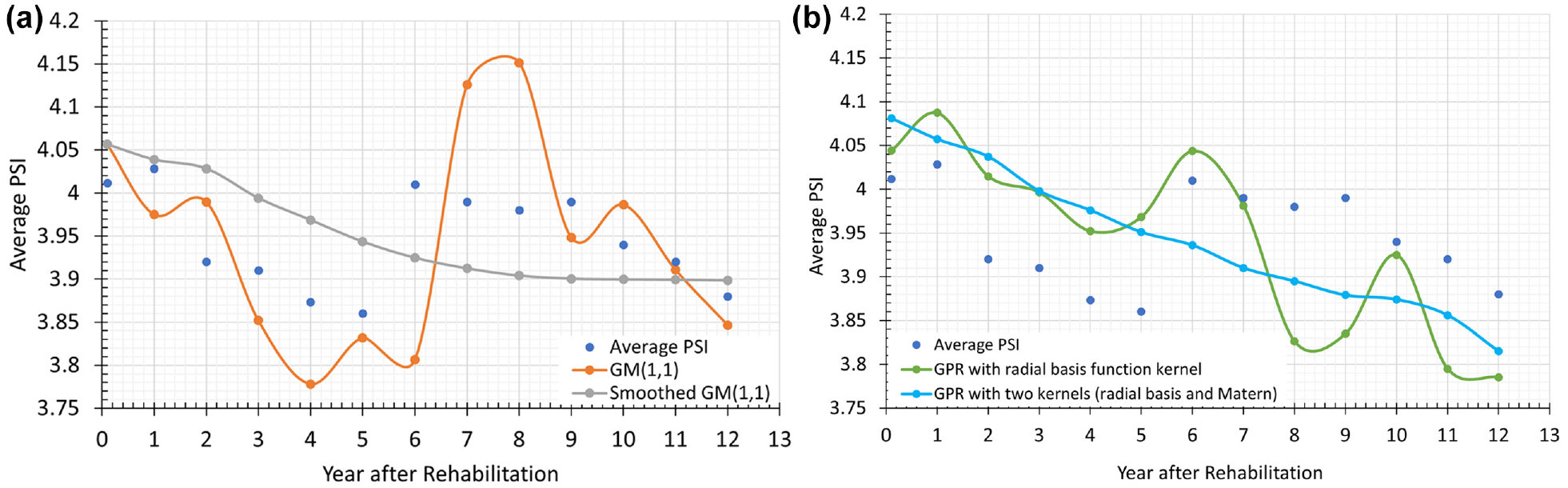
Comparison of GM(1,1) with and without smoothing and GPR with one and two kernels: (a) GM(1,1) model for MR 1–2 in. + OL 400 PSY for asphalt pavement and (b) GPR Model for MR 1–2 in. + OL 400 PSY for asphalt pavement.

The actual versus predicted PSIs and PDIs are shown in Figures 5 to 8. These plots allow for easier assessment and comparison of models’ performance. The predicted range is based on the number of years for which the data are available in the test datasets. The results of GM(1,1) are based on an interval size, $ω$ , of 4 years. That is, four observations are used to predict the next year’s PSI. To estimate year 0’s PSI, we generated four pseudo values by adding Gaussian noise N(0,0.0001) to year 0’s observed PSI and used the model parameters obtained for year 0 (from the training data). In the rolling horizon framework, $k = 4 + 1 = 5$ .

Figure 5.

Comparison of estimated PSI/PDI for asphalt pavement and MR 1–2 in. + OL 400 PSY rehabilitation treatment: (a) comparison of estimated PSI for asphalt pavement and MR 1–2 inches + OL 400 PSY rehabilitation treatment and (b) comparison of estimated PDI for asphalt pavement and MR 1–2 inches + OL 400 PSY rehabilitation treatment.

Figure 6.

Comparison of estimated PSI/PDI for asphalt over concrete pavement and MR 1–2 in. + OL 400 PSY rehabilitation treatment: (a) comparison of estimated PSI for asphalt over concrete pavement and MR 1–2 in. + OL 400 PSY rehabilitation treatment and (b) comparison of estimated PDI for asphalt over concrete pavement and MR 1–2 inches + OL 400 PSY rehabilitation treatment.

Figure 7.

Comparison of estimated PSI/PDI for asphalt pavement and MR 2–4 in. + OL 200 PSY rehabilitation treatment: (a) Comparison of estimated PSI for asphalt pavement and MR 2–4 in. + OL 200 PSY rehabilitation treatment and (b) comparison of estimated PDI for asphalt pavement and MR 2–4 in. + OL 200 PSY rehabilitation treatment.

Figure 8.

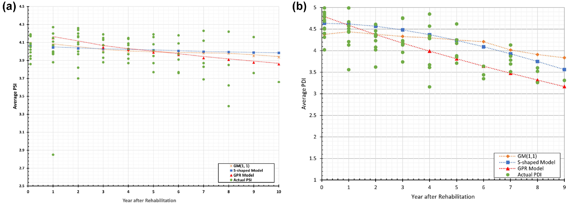
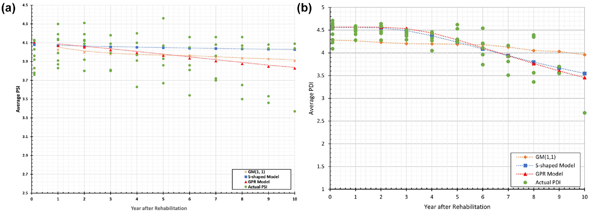
Comparison of estimated PSI/PDI for asphalt over concrete pavement and MR 2–4 in. + OL 200 PSY rehabilitation treatment: (a) Comparison of estimated PSI for asphalt over concrete pavement and MR 2–4 in. + OL 200 PSY rehabilitation treatment and (b) comparison of estimated PDI for asphalt over concrete pavement and MR 2–4 in. + OL 200 PSY rehabilitation treatment.

MR 1–2 in. + OL 400 PSY for Asphalt Pavement

It can be seen in Figure 5 that there is a significant variation in the average PSI and PDI between route segments. For example, two years after an asphalt pavement received the MR 1–2 in. + OL 400 PSY rehabilitation treatment, one segment has an average PSI as low as 3.0 while another segment has an average PSI as high as approximately 4.28. It can be seen visually that the GPR and $GM (1, 1)$ models produced estimates that are closer to one another and they both produced estimates that are lower than the S-shaped model. Based on the MAPE, RMSE, and MAE metrics, $GM (1, 1)$ outperformed GPR and S-shaped models. As shown in Table 5, its MAPE is 4.67, RMSE is 17.02, and MAE is 27.11. A MAPE that is less than 5% indicates that the model is highly accurate ( 31 , 32 ).

Table 5.

Actual versus Predicted PSIs/PDIs for Different Pavement Types and Rehabilitation Methods

Model	MAPE (%)	RMSE (%)	MAE (%)
PSI for MR 1–2 in. + OL 400 PSY for asphalt pavement
S-shaped	5.61	20.3	30.57
GM(1,1)	4.67	17.02	27.11
GPR	4.72	17.91	28.31
PDI for MR 1–2 in. + OL 400 PSY for asphalt pavement
S-shaped	5.74	43.24	37.63
GM(1,1)	4.48	28.76	25.75
GPR	4.62	32.69	29.75
PSI for MR 1–2 in. + OL 400 PSY for asphalt over concrete pavement
S-shaped	4.92	17.39	26.48
GM(1,1)	3.94	14.97	21.47
GPR	3.89	14.78	21.22
PDI for MR 1–2 in. + OL 400 PSY for asphalt over concrete pavement
S-shaped	5.49	27.43	21.86
GM(1,1)	4.97	25.67	19.11
GPR	2.23	25.09	14.75
PSI for MR 2–4 in. + OL 200 PSY for asphalt pavement
S-shaped	5.76	20.96	25.35
GM(1,1)	4.68	16.09	21.54
GPR	4.74	18.31	21.31
PDI for MR 2–4 in. + OL 200 PSY for asphalt pavement
S-shaped	5.71	27.44	14.86
GM(1,1)	4.58	21.02	13.29
GPR	5.23	25.09	14.24
PSI for MR 2–4 in. + OL 200 PSY for asphalt over concrete pavement
S-shaped	4.44	17.21	22.10
GM(1,1)	3.11	12.23	15.53
GPR	2.69	10.61	14.52
PDI for MR 2–4 in. + OL 200 PSY for asphalt over concrete pavement
S-shaped	9.14	36.26	28.98
GM(1,1)	6.53	33.65	24.83
GPR	3.76	29.33	21.25

Note: PSI = pavement serviceability index; PDI = pavement distress index; MAPE = mean absolute percentage error; RMSE = root mean square error; MAE = mean absolute error; MR = rehabilitation method; OL 200/400 PSY = 200/400 pounds per square yard overlay; GM = grey system model; GPR = Gaussian process regression.

MR 1–2 in. + OL 400 PSY for Asphalt over Concrete Pavement

Similar to the results shown in Figure 5, there is a significant variation in the average PSI and PDI between route segments for asphalt over concrete pavements that received MR 1–2 in. + OL 400 PSY rehabilitation treatment as shown in Figure 6. By inspection, it can be seen that the GPR model predicted the fastest deterioration rate, followed by $GM (1, 1)$ . The S-shaped model predicted a nearly flat trend which is highly improbable. That is, it is unlikely for the functional condition of a pavement to remain the same 10 years after being rehabilitated. Based on the MAPE, RMSE, and MAE metrics, GPR outperformed $GM (1, 1)$ and S-shaped models. As shown in Table 5, its MAPE is 3.89, RMSE is 14.78, and MAE is 21.22. The values of all three performance metrics are lower compared with the MR 1–2 in. + OL 400 PSY for asphalt pavement model. Thus, it can be inferred that this model has better predictive power.

MR 2–4 in. + OL 200 PSY for Asphalt Pavement

The actual and predicted PSIs and PDI for asphalt pavements after receiving the MR 2–4 in. + OL 200 PSY rehabilitation treatment is shown in Figure 7. Similar to the trends shown in Figure 6, it can be seen that the GPR model predicted faster pavement deterioration compared with $GM (1, 1)$ and S-shaped models. The S-shaped model once again predicted nearly constant PSI values. Unlike previous findings, no model outperformed the others on all three metrics. Based on MAPE and RMSE, $GM (1, 1)$ yielded the best performance. However, based on MAE, GPR is the better model. RMSE is more sensitive to observations that are further from the mean than MAE. Thus, depending on the preference of the agency, either $GM (1, 1)$ or GPR would provide better estimates than the S-shaped model.

MR 2–4 in. + OL 200 PSY for Asphalt over Concrete Pavement

The actual and predicted PSIs and PDI for asphalt over concrete pavements after receiving the MR 2–4 in. + OL 200 PSY rehabilitation treatment are shown in Figure 8. For this combination of pavement type and rehabilitation method, all three models produced estimates that are close to one another. A close inspection shows that the $GM (1, 1)$ predicted the fastest pavement deterioration rate, followed by the GPR, and then the S-shaped model. The S-shaped model is most likely to produce incorrect estimates based on its nearly constant slope, meaning pavement functional condition remains the same year after year. Based on all three metrics, the GPR model is considered the best model.

Discussion

The model validation results indicate that both the $GM (1, 1)$ and GPR models are superior to the S-shaped model based on MAPE, RMSE, and MAE metrics. The S-shaped model is particularly problematic in three out of the four cases, producing a nearly flat slope for pavement deterioration over time, which is unrealistic. When using MAE as a performance metric, GPR is the better model in three out of four cases, with the exception being the case involving asphalt pavement with MR 1–2 in. + OL 400 PSY rehabilitation treatment. However, when using MAPE and RMSE as the performance metrics, the GPR model outperforms the $GM (1, 1)$ model in predicting conditions for asphalt over concrete (i.e., composite) pavements, while the $GM (1, 1)$ model is superior in predicting conditions for asphalt pavements.

Aside from their methodological differences, there are two main practical differences between the S-shaped, GM(1,1), and GPR models. The first is that the GPR and GM(1,1) models do not necessarily predict a higher rate of deterioration as the pavement gets older as is the case with S-shaped model. The second practical difference is that the GM(1,1) model runs in a rolling horizon manner, and thus, it makes use of the latest available data. As such, it is better at capturing potential abrupt changes in pavement conditions. From an implementation perspective, the S-shaped model is the easiest to implement; it can be set up and run on a spreadsheet. On the other hand, a GPR or GM(1,1) model will require the use of a programming and numeric computing platform such as MATLAB or Python.

Summary and Conclusions

This study evaluated the performance of three different approaches to predict pavement functional conditions (PSI) and pavement structural conditions (PDI) from South Carolina. The aim was to determine whether a semi-parametric model (GM) and a non-parametric model (GPR) outperform the traditional parametric model (S-shaped). After training the models on the training datasets, they were then tested on separate test datasets. The prediction results for both PSI and PDI indicated that the $GM (1, 1)$ model outperformed both the GPR model and S-shaped model for asphalt pavements under both types of rehabilitation treatments, based on the performance metrics MAPE and RMSE. However, for PSI and if MAE were to be used as the performance metric, then GPR outperformed the $GM (1, 1)$ model for the MR 2–4 in. + OL 200 PSY treatment. For asphalt over concrete pavements under both types of rehabilitation treatments, GPR performed best across all performance metrics. By utilizing a rolling horizon approach with the proposed GM, the prediction results indicated that it was able to capture the nonlinear trends in the PSI data well and make accurate predictions with just four prior observations. The key takeaway from this study is that the traditional S-shaped model produced poor estimates and unrealistic projections in three out of four cases. Therefore, the study recommends using more advanced techniques such as GPR or GM.

The study demonstrated the applicability and effectiveness of using $GM (1, 1)$ and GPR models to predict pavement conditions with a relatively small sample size. In their original forms, neither the $GM (1, 1)$ nor the GPR model is capable of producing monotonically decreasing trends. However, this functionality was enabled by incorporating a smoothing function in the $GM (1, 1)$ model and by using a combination of two kernels for the GPR model. Future work in this area could aim to identify specific factors related to pavement types and rehabilitation treatment types that make a GM more suitable than GPR and vice-versa. Another area that needs further investigation is the spatial interval. In this work, an average PSI or PDI was used to represent the condition of the pavement for the entire rehabilitation project. Smaller intervals may be needed to detect very rough sections to assist those DOTs that use indices to trigger work needs.

Footnotes

Authors Contribution

The authors confirm contribution to the paper as follows: study conception and design: J. Wang, G. Comert, N. Begashaw, N. Huynh, A. Kouyate, R. Mullen, S. Gassman, and C. Pierce; data collection: A. Kouyate; analysis and interpretation of results: J. Wang, G. Comert, N. Huynh, and A. Kouyate; draft manuscript preparation: J. Wang, G. Comert, N. Begashaw, N. Huynh, A. Kouyate, R. Mullen, S. Gassman, and C. Pierce. All authors reviewed the results and approved the final version of the manuscript.

Declaration of Conflicting Interests

The author(s) declared no potential conflicts of interest with respect to the research, authorship, and/or publication of this article.

Funding

The author(s) disclosed receipt of the following financial support for the research, authorship, and/or publication of this article: The study was supported by the South Carolina Department of Transportation (SCDOT) [grant number: SPR No. 743].

ORCID iDs

Jing Wang

Gurcan Comert

Nathan Huynh

Amara Kouyate

Sarah Gassman

Any opinions, findings, conclusions, or recommendations expressed in this paper are those of the authors and do not necessarily reflect the views of the SCDOT.

References

Meegoda

J. N.

Gao

Roughness Progression Model for Asphalt Pavements Using Long-Term Pavement Performance Data. Journal of Transportation Engineering, Vol. 140, No. 8, 2014, p. 04014037.

Chang

C.-M.

Baladi

G. Y.

Wolff

T. F.

Using Pavement Distress Data to Assess Impact of Construction on Pavement Performance. Transportation Research Record: Journal of the Transportation Research Board, 2001. 1761: 15–25.

David

Geiger

Memo: Pavement Preservation Definitions—Design Analysis. Washington, D.C., 2005https://www.fhwa.dot.gov/pavement/preservation/091205.cfm.

Kouyate

Evaluation of a Trigonometric Grey Model for Estimating and Predicting Pavement Condition. Master thesis. University of South Carolina, Columbia, SC, 2021.

Montenegro

On Sample Size and Precision in Ordinary Least Squares. Journal of Applied Statistics, Vol. 28, No. 5, 2001, pp. 603–605.

Zhang

Xiong

A Methodology for Evaluating Micro-Surfacing Treatment on Asphalt Pavement Based on Grey System Models and Grey Rational Degree Theory. Construction and Building Materials, Vol. 150, 2017, pp. 214–226.

Rasmussen

C. E.

Williams

C. K. I.

Gaussian Processes for Machine Learning. Vol. 2. No. 3. Cambridge, MA: MIT press, 2006.

Kleijnen

J. P.

Kriging Metamodeling in Simulation: A Review. European Journal of Operational Research, Vol. 192, No. 3, 2009, pp. 707–716.

Madarshahian

Balaram

Ahmed

Huynh

Siddiqui

C. K.

Ferguson

Analysis of Injury Severity of Work Zone Truck-Involved Crashes in South Carolina for Interstates and Non-Interstates. Sustainability, Vol. 15, No. 9, 2023, p. 7188.

10.

Shahin

M. Y.

Nunez

M. M.

Broten

M. R.

Carpenter

S. H.

Sameh

New Techniques for Modeling Pavement Deterioration. Transportation Research Record, 1123, 40–46, Washington. D.C., 1987.

11.

Abaza

K. A.

Deterministic Performance Prediction Model for Rehabilitation and Management of Flexible Pavement. International Journal of Pavement Engineering, Vol. 5, No. 2, 2004, pp. 111–121.

12.

Prozzi

J. A.

Hong

Transportation Infrastructure Performance Modeling through Seemingly Unrelated Regression Systems. Journal of Infrastructure Systems, Vol. 14, No. 2, 2008, pp. 129–137.

13.

Rahman

M. M.

Uddin

M. M.

Gassman

S. L.

Pavement Performance Evaluation Models for South Carolina. KSCE Journal of Civil Engineering, Vol. 21, 2017, pp. 2695–2706.

14.

Luo

Chou

E. Y.

Pavement Condition Prediction Using Clusterwise Regression. Transportation Research Record: Journal of the Transportation Research Board, 2006. 1974: 70–77.

15.

George

Rajagopal

Lim

Models for Predicting Pavement Deterioration. Transportation Research Record, Vol. 1215, Washington, D.C., 1989, pp. 1–4.

16.

Chan

P. K.

Oppermann

M. C.

S.-S.

North Carolina’s Experience in Development of Pavement Performance Prediction and Modeling. Transportation Research Record: Journal of the Transportation Research Board, 1997. 1592: 80–88.

17.

Gulen

Zhu

Weaver

Shan

Flora

Development of Improved Pavement Performance Prediction Models for the Indiana Pavement Management System. Joint Transportation Research Program, West Lafayette, IN, 2001.

18.

Kim

S.-H.

Kim

Development of Performance Prediction Models in Flexible Pavement Using Regression Analysis Method. KSCE Journal of Civil Engineering, Vol. 10, 2006, pp. 91–96.

19.

Bai

Sun

Pavement Deterioration Modeling and Prediction for Kentucky Interstate and Highways. Proc., IIE Annual Conference, Institute of Industrial and Systems Engineers (IISE), Montreal, QC, Canada, 2014, p. 993.

20.

Tsai

J. Y.

Wang

C. R.

Georgia Concrete Pavement Performance and Longevity. Georgia Department of Transportation, Atlanta, GA, 2012.

21.

Tang

Xiao

Monthly Attenuation Prediction for Asphalt Pavement Performance by Using GM (1, 1) Model. Advances in Civil Engineering, Vol. 2019, 2019, p. 9274653.

22.

Zhang

D.-B.

Zhang

Prediction Method of Asphalt Pavement Performance and Corrosion Based on Grey System Theory. International Journal of Corrosion, Vol. 2019, 2019, p. 2534794.

23.

J.-C.

Shen

D.-H.

Development of Pavement Permanent Deformation Prediction Model by Grey Modelling Method. Civil Engineering and Environmental Systems, Vol. 22, No. 2, 2005, pp. 109–121.

24.

Heyns

De Villiers

J. P.

Heyns

P. S.

Consistent Haul Road Condition Monitoring by Means of Vehicle Response Normalisation with Gaussian Processes. Engineering Applications of Artificial Intelligence, Vol. 25, No. 8, 2012, pp. 1752–1760.

25.

Stantec Consulting. South Carolina HPMA Index Models, 2014. https://imlive.s3.amazonaws.com/South%20Carolina/ID32410561292247916663692960757358151668/Attachment%20A.pdf.

26.

Ju-Long

Control Problems of Grey Systems. Systems & Control Letters, Vol. 1, No. 5, 1982, pp. 288–294.

27.

Liu

Lin

Grey Information: Theory and Practical Applications. Springer Science Business Media New York City, NY, 2006.

28.

Zeng

Prediction of Building Electricity Usage Using Gaussian Process Regression. Journal of Building Engineering, Vol. 28, 2020, p. 101054.

29.

Chen

Mastin

Sigmoidal Models for Predicting Pavement Performance Conditions. Journal of Performance of Constructed Facilities, Vol. 30, No. 4, 2016, p. 04015078.

30.

Uwanuakwa

I. D.

Ali

S. I. A.

Hasan

M. R. M.

Akpinar

Sani

Shariff

K. A.

Artificial Intelligence Prediction of Rutting and Fatigue Parameters in Modified Asphalt Binders. Applied Sciences, Vol. 10, No. 21, 2020, p. 7764.

31.

Lewis

C. D.

Industrial and Business Forecasting Methods: A Practical Guide to Exponential Smoothing and Curve Fitting. Butterworth Scientific, London, 1982.

32.

Moreno

J. J. M.

Pol

A. P.

Abad

A. S.

Blasco

B. C.

Using the R-MAPE Index as a Resistant Measure of Forecast Accuracy. Psicothema, Vol. 25, No. 4, 2013, pp. 500–506.