Multi-Type Traffic Conflict Identification at Signalized Intersections Based on LiDAR Point Cloud

Abstract

Traffic conflicts have been widely used for proactive road safety evaluation, and this study develops methods to automatically identify different types of traffic conflict based on LiDAR point cloud data. With 10 h of data collected from a signalized intersection in Harbin, China, trajectories of motorized vehicles, bicycles, and pedestrians were extracted, and methods to handle the issues of trajectory discontinuity, type identification error, and same object with different trajectories were developed. Traffic conflicts between right-turn vehicles and through vehicles, between right-turn vehicles and left-turn vehicles, and between right-turn vehicles and pedestrians were considered, and detailed procedures for calculating the conflict indicators (i.e., time to collision [TTC] and post encroachment time [PET]) of different types were proposed. The identified traffic conflicts were also compared with the ones that were identified manually. A total of 5,352 and 1,366 traffic conflicts were identified by PET ≤ 4 s and TTC ≤ 4 s, respectively. The majority were during the through phase, and traffic conflicts between right-turn vehicles and through vehicles were the most common, followed by conflicts between right-turn vehicles and vulnerable road users (i.e., cyclists and pedestrians).The proposed automatic method considers the actual sizes of involved road users and thus leads to more accurate conflict indicator calculation, with an average accuracy over 90%.

Keywords

data mining safety safety performance and analysis traffic conflict LiDAR

Signalized intersections have been widely recognized as hazardous locations because of their large traffic volume, frequent stop-and-go traffic, and complex conflicting movements ( 1 – 3 ). For example, statistics show that 22% of traffic crashes in the U.S. occur at intersections ( 4 ). In Canada, crashes at intersections caused more than 30% of road traffic accident (RTA) deaths and 40% of RTA serious injuries, and most of the injuries in urban areas occurred at signalized intersections ( 5 , 6 ). Traditionally, the safety analysis of signalized intersections relies heavily on historical crash records, which have well-known availability and quality problems such as under-reporting, small sample size, and unobserved heterogeneity ( 7 ). These issues have led to the emergence of “traffic conflict techniques.”

Traffic conflict techniques have gained great popularity in recent years, and they have been widely used in traffic safety evaluation, before–after safety analysis, real time safety prediction, and some other safety areas ( 8 ). A traffic conflict is usually defined as “an observable situation in which two or more road users approach each other in space and time to such an extent that there is a risk of collision if their movements remain unchanged” ( 9 ). Therefore, to define and measure the severity of traffic conflicts, different conflict indicators have been proposed, of which temporal/spatial proximity indicators are the most common ( 10 ). A recent review study summarized relevant articles and identified 38 proximal indicators; examples include time to collision (TTC), modified time to collision (MTTC), and post encroachment time (PET) ( 11 ). To objectively and accurately calculate these indicators, it is necessary to obtain trajectories of involved road users.

The majority of trajectory extraction methods in traffic conflict research are based on video recordings and computer vision techniques. Guido et al. compared different conflict indicators obtained from video capture data, and processed the data on a frame by frame basis to extract trajectories using Adobe Premiere software ( 12 ). Oh et al. developed an automatic traffic conflict detection system based on image tracking ( 13 ). The system contained general tracking steps (i.e., background substraction, moving vehicle segmentation and noise removal, and individual identification labeling) and conflict detection steps (i.e., automatic detection lane calculation, traffic conflict decision algorithm, and results display). There are also some well-developed video-based tools to extract road user trajectories and identify traffic conflicts, such as the semi-automated tool T-Analyst developed at Lund University and a fully automated traffic conflict identification tool developed at the University of British Columbia ( 14 – 16 ). Using video data and computer vision techniques for trajectory extraction and conflict identification has several advantages, such as low cost and high efficiency, especially with the advancement of artificial intelligence techniques ( 10 , 17 , 18 ). However, the quality of extracted trajectories could be significantly affected by the prevailing traffic conditions, such as congested traffic, and environment conditions, such as illumination variations and shadow changes.

To overcome the limitations of video data, light detection and ranging (LiDAR) technology has been employed for road user identification and trajectory extraction in recent years. The main processes involved in the LiDAR data process include background filtering, object clustering, object classification, and tracking ( 19 , 20 ). The processes are similar to those based on video data. The difference is that LiDAR data are point clouds generated by multi-channel laser instead of images ( 21 ). Tarko et al. developed a roadside LiDAR system, T-Scan, to collect trajectories of different types of road user for traffic conflict analysis ( 22 ). Wu et al. investigated vehicle–pedestrian conflicts using trajectories extracted from a roadside LiDAR sensor ( 23 , 24 ). Lv et al. and Vasudevan et al. also developed vehicle–pedestrian conflict identification methods using trajectories extracted from the roadside LiDAR sensor ( 25 , 26 ). Bhattarai et al. proposed the use of the LiDAR sensor to detect rear-end conflicts at signalized intersections ( 27 ). Other than the studies directly connected to road safety analysis, there are also studies that aimed at only object detection and tracking by using the LiDAR sensor ( 28 – 31 ).

In general, previous studies have shown that using LiDAR sensors for road user detection and tracking is insusceptible to changes in illumination, weather, and shadow, could provide high resolution micro traffic data, and has improved detection range and accuracy ( 19 , 28 ). Because of these advantages, the LiDAR technique has seen an increasing application in traffic conflict studies. However, previous studies mainly focused on a certain type of conflict or a certain conflict indicator, and a systematic method for identifying traffic conflicts of different types and with different indicators is still missing. To bridge these gaps, this study conducts a multi-type traffic conflict identification at a signalized intersection based on the LiDAR point cloud.

The rest of the study is organized as follows. The next section presents the acquisition of LiDAR point cloud data. Classification of conflict types, calculation of conflict indicators, and determination of thresholds are shown in the section after that. The penultimate section presents the results of identification, and discussions. The conclusions are presented in the final section.

Data Collection

An RS-Ruby Lite LiDAR sensor produced by RoboSense was used for data collection. The point cloud data were collected at a signalized intersection in Harbin, China, on October 8, 2021. The frame rate of LiDAR is 10 frames per second. The main road at the intersection is a two-way ten-lane road and the branch is a two-way, six-lane road. The signal timing of the intersection in is a segmented fixed signal timing with five phases. The LiDAR was placed at the southwest corner of the intersection. The top view of the intersection, the phases of this intersection, and the position where the LiDAR was placed are shown in Figure 1. To cover both the peak hour and off-peak hour and to ensure the amount of data is large enough for the following analysis, a total of 10 h of data (i.e., 7:00–17:00) were collected.

Figure 1.

Top view of the intersection.

The raw LiDAR points were first processed with the Software Development Kit (SDK) developed by RoboSense. SDK combines traditional geometric-based approaches and deep learning approaches to detect, classify, and track the objects. The detection function categorizes the points into clusters and defines the clusters as detected objects with a 3D bounding box. The classification function distinguishes types of detected objects—the types include passenger cars, buses, trucks, non-motorized vehicles, pedestrians, and so forth. The tracking function identifies the same object in continuous data frames and generates the speed and trajectory for each detected object. The processed data are illustrated in Figure 2. The statistics of the traffic data are shown in Table 1.

Figure 2.

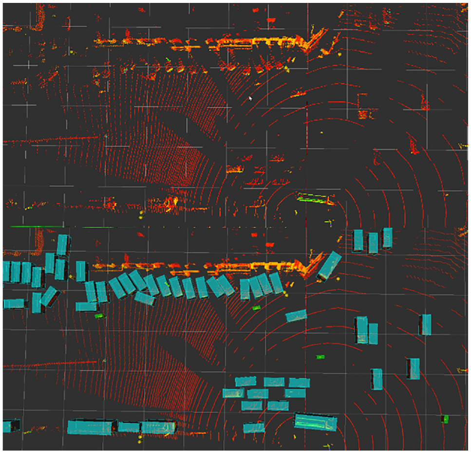
Raw (top) and processed (bottom) LiDAR points.

Table 1.

Statistics of Hourly Traffic Volume

	Motorized vehicle (vph)			Non-motorized vehicle (vph)	Pedestrian (pph)
	Through	Right-turn	Left-turn	Non-motorized vehicle (vph)	Pedestrian (pph)
Eastern approach
Minimum	452	263	88	71	72
Mean	572	464	157	344	363
Maximum	678	567	212	467	441
Western approach
Minimum	505	198	121	67	36
Mean	613	312	165	78	56
Maximum	715	478	244	99	97
Southern approach
Minimum	475	132	113	174	31
Mean	577	154	198	231	57
Maximum	633	221	299	375	82
Northern approach
Minimum	271	234	189	116	66
Mean	313	312	261	176	250
Maximum	337	378	448	237	316

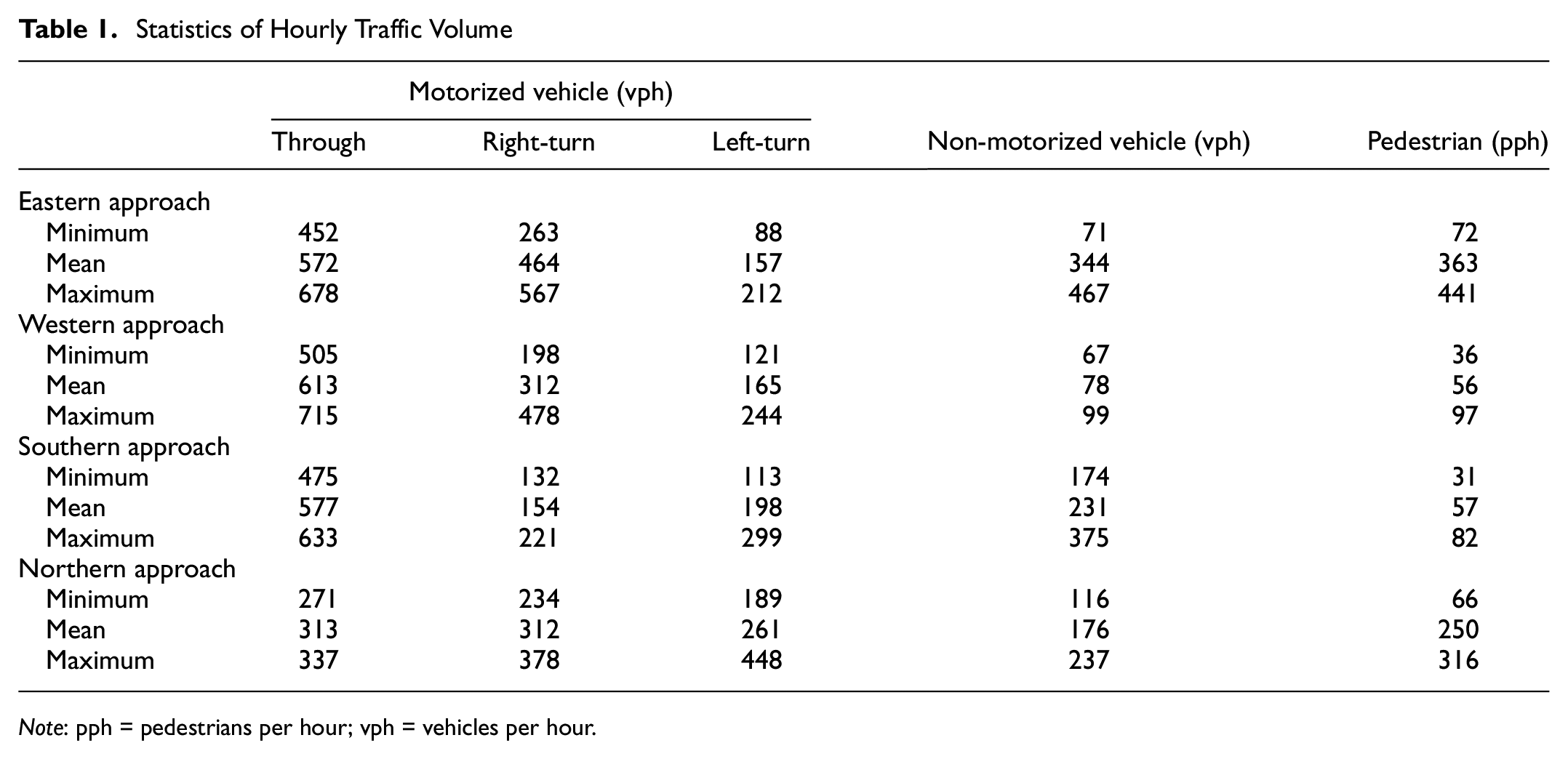
Note: pph = pedestrians per hour; vph = vehicles per hour.

Methodology

Data Processing

The trajectory data of objects extracted from the original point clouds include the ID (track_id), the coordinates of the center point (center_x, center_y), the type (car, truck_bus, pedestrian, bicycle), the size of the bounding box (size_x, size_y), and the track extraction time (timestamp). After visualizing the trajectory data, the following issues are found: 1) Some trajectories are not discontinuous; 2) Object type identification error exists; 3) One object has several different trajectories.

Trajectory Discontinuity

Because of the obstruction between vehicles, some trajectories are discontinuous, as shown in Figure 3a. In this case, the ID, the coordinates of the center point, the type, and the size of the bounding box are all null values. For these discontinuous trajectories, their ID and target type are filled with the values right before the null values. The coordinates of the centroid and the size of the bounding boxes are derived by polynomial interpolation. When polynomial interpolation cannot be derived, linear interpolation is used instead. Figure 3 shows the trajectories before and after the interpolation.

Figure 3.

Trajectories (a) before and (b) after the interpolation.

Type Identification Error

For the wrongly identified objects, the types and the coordinates of the bounding box need to be corrected. In general, there are two cases: 1) misidentification between truck/bus and car and 2) misidentification between bicycle and pedestrian.

The misidentification between truck/bus and car usually happens in individual trajectories, where the type of the object would change suddenly while its IDs remain the same. Moreover, the falsely identified type only lasts for a few frames. Therefore, after grouping, the object type with fewer occurrences is replaced by the one with more occurrences. It is also noted that, because of the measurement error in LiDAR points, the bounding box of the same object may change over time, and their average value is taking as the size of the object.

The misidentification between bicycle and pedestrian is because of their small size and similar quantity of LiDAR points. Since type identification is mainly based on the size of objects, the similar quantity of LiDAR points usually leads to a similar size. To distinguish these two types of object, their average speeds were considered. The distribution of pedestrians’ and bicycles’ speeds is shown in Figure 4. It can be found that the speeds of pedestrians are generally less than 2 m/s while the speeds of bicycles are greater than 2 m/s. Therefore, 2 m/s is selected as the boundary for classification. The trajectories with an average speed less than 2 m/s are marked as a pedestrian, and otherwise as a bicycle.

Figure 4.

Speeds of pedestrians and bicycles.

Same Object with Different Trajectories

When an object is blocked by another object for relatively long time, it would come up as a new object, leading to different trajectories for the same object. To solve this problem, the polynomial fitting method is employed. The segmented trajectories within a signal cycle were fitted by the quadratic polynomial function, as shown in Figure 5. The trajectories located on the same polynomial curve were identified as the same trajectory. An example of the trajectory stitching is shown in Figure 6. The discontinuity issue is then fixed by the interpolation presented in Trajectory Discontinuity.

Figure 5.

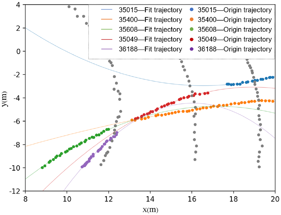
Trajectories fitted by the quadratic polynomial.

Figure 6.

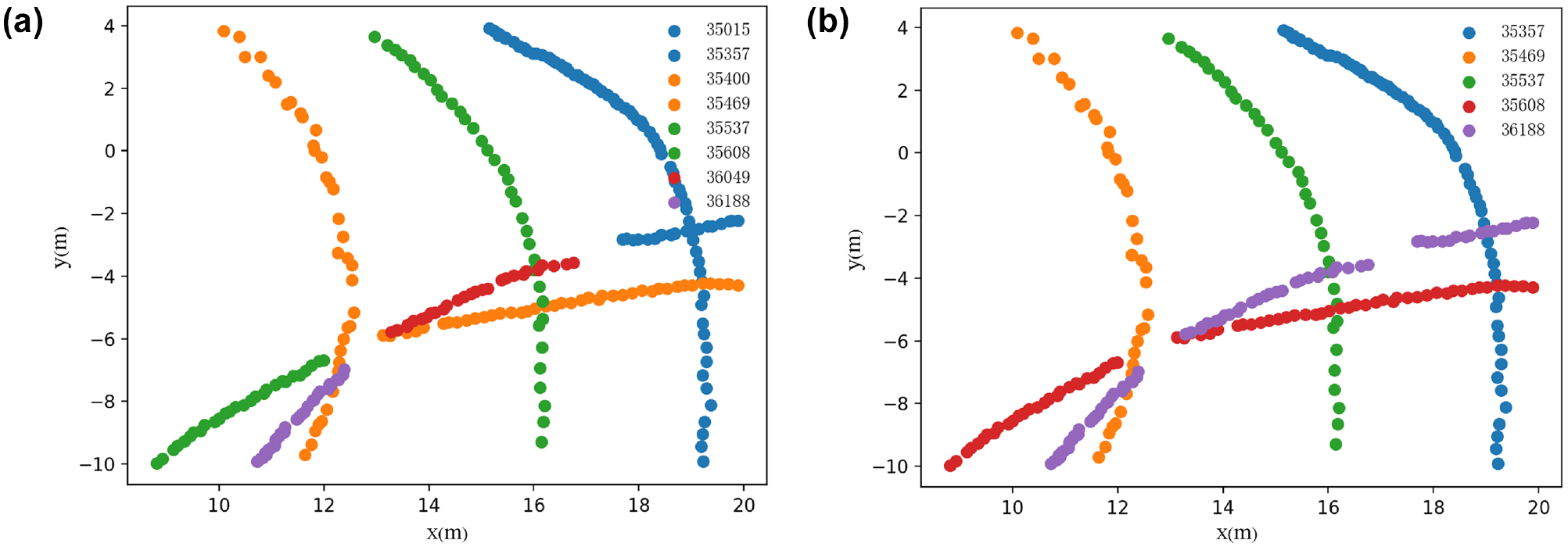
Trajectories (a) before and (b) after the polynomial fitting.

Conflict Identification

Conflict Type Selection

A four-approach intersection has, at most, 32 conflicting points between different vehicle flows, and 24 conflicting points between vehicle flows and pedestrian flows. For the investigated signalized intersection with five phases, there are only eight conflicting points between vehicles and eight conflicting points between vehicles and pedestrians, as shown in Figure 7. To be specific, the traffic conflicts considered in this study are: conflicts between right-turn vehicles and through vehicles, conflicts between right-turn vehicles and left-turn vehicles, and conflicts between right-turn vehicles and pedestrians. Note that the vehicles include motorized vehicles and bicycles.

Figure 7.

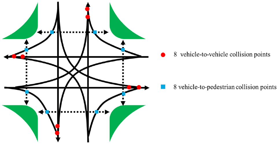
Distribution of conflict points at the intersection.

Conflict Indicator Calculation

To measure the severity of traffic conflicts, two widely used indicators, PET and TTC, are used. TTC is the time remaining before a collision occurs if the involved road users continue to maintain their speed and trajectory ( 32 ). PET is the time difference between a vehicle leaving a potential collision point and another vehicle arriving at the collision point ( 33 ). It is noted that the TTC exists only when there is a collision course (i.e., the two road users would collide if they retain their speeds and directions) while the PET exists when the trajectories of involved road users overlap.

To calculate the indicators, a procedure was proposed with three steps: bounding box-related data calculation, potential conflict identification, and conflict indicator calculation. Compared with previous studies that simplified the object into a single point (e.g., central point) for subsequent conflict identification and indicator extraction, this procedure considers the size of the volume occupied by the object in the 2D plane, which enables more accurate calculation of interested conflict indicators ( 25 , 26 ). It is noted that the improvement in accuracy is at the cost of longer computational time, especially in calculating the bounding box and identifying the potential conflicts.

Step 1: bounding-box-related data calculation

To accurately calculate the conflict indicators, the four vertices of the bounding box, the equations of the lines where the four sides are located, and the direction of the objects need to be calculated (see Figure 8).

Figure 8.

Diagram of the bounding box.

Firstly, the equation of the line L5 (as shown in Figure 8) is calculated. Let the coordinates of the object centroid at time t₁ be (Ti_x, Ti_y) and the coordinates at time t₂ be (Tii_x, Tii_y), where t₁ and t₂ are two adjacent frames in the timestamp. Based on the two coordinates, equations of the line that connects the two centroid and the speed of the object could be derived as follows:

ax + by + c = 0

(1)

y = kx + d

(2)

v = \sqrt{{(\frac{Tii_x - Ti_x}{0.1})}^{2} + {(\frac{Tii_y - Ti_y}{0.1})}^{2}}

(3)

a = Tii_y - Ti_y

(4)

b = Ti_x - Tii_x

(5)

c = Ti i_x \times Ti_y - Ti_x \times Tii_y

(6)

k = {\begin{matrix} - \frac{a}{b}, b \neq 0 \\ non - existent, b = 0 \end{matrix}

(7)

d = {\begin{matrix} - \frac{c}{b}, b \neq 0 \\ non - existent, b = 0 \end{matrix}

(8)

where

a, b, and c = the coefficients of the general equation of the line,

k and d = the coefficients of the intercept equation of the line, and

v = the speed of the object.

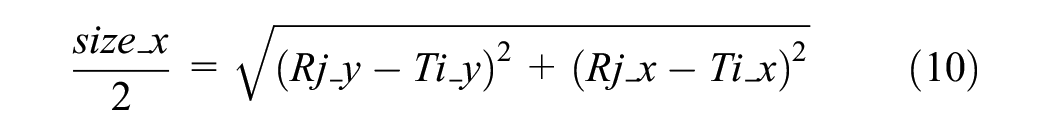
Secondly, the coordinates of A, B, C, D, E, and F (as shown in Figure 8) are calculated. The method for calculating point E and vertices A and B is illustrated, and point F and vertices C and D are calculated in the same way. As the interval between t₁ and t₂ is very short (i.e., 0.1 s), it can be assumed that the moving direction of the object remains unchanged during this time. Therefore, the slope of the line connecting G and E is approximately equal to the slope of the line L5, and point G is the midpoint of the line segment EF. In this way, the coordinates of the point E can be derived, as Equations 9 and 10. For the coordinates of points A and B, knowing that E is the midpoint of line AB, and line AB is perpendicular to line L5, according to Equations 11 and 12, the coordinates of points A and B can be calculated.

k = \frac{Rj_y - Ti_y}{Rj_x - Ti_x}

(9)

\frac{size_x}{2} = \sqrt{{(Rj_y - Ti_y)}^{2} + {(Rj_x - Ti_x)}^{2}}

(10)

where

Rj_x = the horizontal coordinate of point E(j = 1) and F(j = 2),

Rj_y = the vertical coordinate of point E(j = 1) and F(j = 2), and

size_x = the length of the bounding box.

- \frac{1}{k} = \frac{Sn_y - R 1_y}{Sn_x - R 1_x}

(11)

\frac{size_y}{2} = \sqrt{{(Sn_y - R 1_y)}^{2} + {(Sn_x - R 1_x)}^{2}}

(12)

where

Sn_x = the horizontal coordinate of point A (n = 1) and B (n = 2), and

Sn_y = the vertical coordinate of point A (n = 1) and B (n = 2).

Lastly, the equations of the lines L1, L2, L3, and L4 are calculated. Taking the method of solving the lines L2 and L3 as an example, according to the following conditions: 1) L2 is perpendicular to line L5 and 2) point E is on line L2, the equation of line L2 is easily obtained, as follows:

H_2 X + L_2 Y + J_2 = 0

(13)

- \frac{H_2}{L_2} = - \frac{1}{k}

(14)

H_2 \times R 1_x + L_2 \times R 1_y + J_2 = 0

(15)

where

H_2, L_2, and J_2 = the coefficients of the general equation of line L2.

According to the remaining conditions: 1) L3 is parallel to line L5 and 2) the distance from line L3 to L5 is half the width of the bounding box, the equation of the straight line L3 can be easily obtained, as follows:

H_3 X + L_3 Y + J_3 = 0

(16)

\frac{H_3}{a} = \frac{L_3}{b}

(17)

\frac{size_y}{2} = \frac{| J_3 - c |}{\sqrt{a^{2} + b^{2}}}

(18)

where

H_3, L_3, and J_3 = the coefficients of the general equation of line L3.

Step 2: potential conflict identification

To identify whether the two objects P and Q are conflicting each other, it is necessary to judge whether the bounding boxes of the two objects overlap or intersect. This is done by bringing the vertices’ coordinates of one object into the equations of two pairs of parallel sides (i.e., L1, L2, L3, L4 in Figure 8) of the other object, respectively arriving at W1, W2, V1, and V2, which are:

W 1 = H_1 M + L_1 N + J_1

(19)

W 2 = H_2 M + L_2 N + J_2

(20)

V 1 = H_3 M + L_3 N + J_3

(21)

V 2 = H_4 M + L_4 N + J_4

(22)

where

(M, N) = the vertices’ coordinates of one object, and

H_i (i = 1, 2, 3, 4), L_j (j = 1, 2, 3, 4), and J_k (k = 1, 2, 3, 4) = the coefficients of the equations of two pairs of parallel sides of the other object.

Then, whether potential conflict exists can be judged according to the positive or negative results. The detailed procedure of potential conflict identification is shown in Figure 9.

Figure 9.

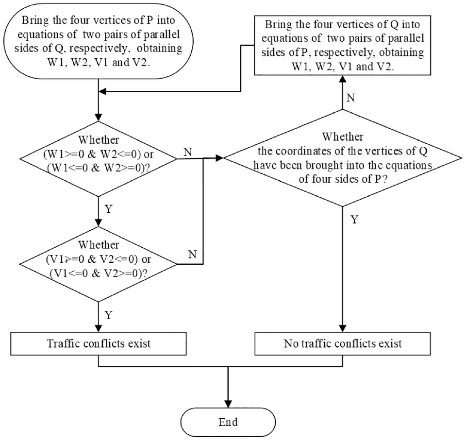
Procedure of potential conflict identification.

Step 3: conflict indicator calculation

For the objects with potential conflicts, their PET and TTC are calculated. To facilitate the calculation, only indicator values less than 4 s are considered. For two objects from different directions passing the conflict area one after another within 4 s, the PET or TTC value is calculated. Otherwise, the operation moves forward with 0.1 s increment along the timestamp. Figure 10 presents a schematic diagram of the PET and TTC calculation for a through vehicle and a right-turn vehicle, and the same calculation method applies for other types of conflict.

Figure 10.

Schematic diagram of (a) post encroachment time (PET) and (b) time to collision (TTC) calculation.

Results and Discussion

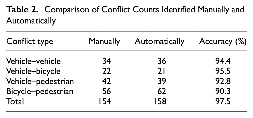
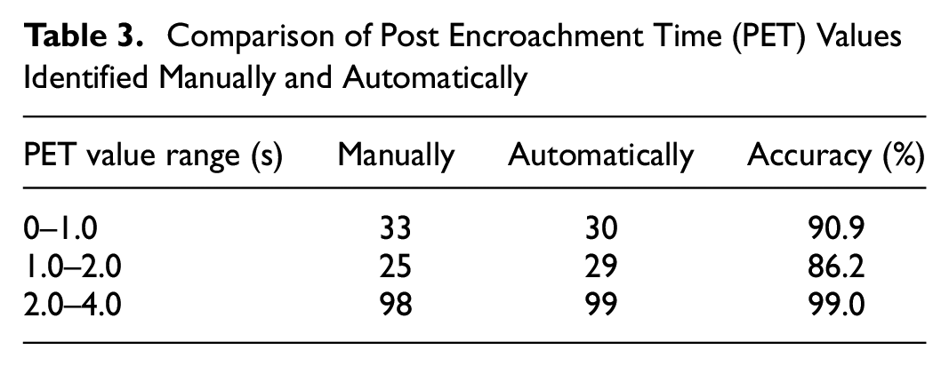
A Python code was developed to automatically identify conflicts, based on the method described above. To evaluate the performance of the proposed method, the extracted conflicts were compared with the ones identified manually. One hour of data is chosen to perform such tests, in which only the conflicts between through vehicles and right-turn vehicles on the east exit were considered. Meanwhile, only PET was considered in this process. The comparison results are shown in Tables 2 and 3. Table 2 shows the differences in counts of traffic conflicts identified manually and automatically, and, in total, the accuracy is as high as 97.5%. Table 3 shows the differences in PET values, and the accuracies for 0–1.0 s, 1.0–2.0 s, and 2.0–3.0 s are 90.9%, 86.2%, and 99.0%, respectively. In general, it can be found that the proposed method performs well. The error is mainly caused by the imprecise coordinates of the object center point and the size of the bounding box.

Table 2.

Comparison of Conflict Counts Identified Manually and Automatically

Conflict type	Manually	Automatically	Accuracy (%)
Vehicle–vehicle	34	36	94.4
Vehicle–bicycle	22	21	95.5
Vehicle–pedestrian	42	39	92.8
Bicycle–pedestrian	56	62	90.3
Total	154	158	97.5

Table 3.

Comparison of Post Encroachment Time (PET) Values Identified Manually and Automatically

PET value range (s)	Manually	Automatically	Accuracy (%)
0–1.0	33	30	90.9
1.0–2.0	25	29	86.2
2.0–4.0	98	99	99.0

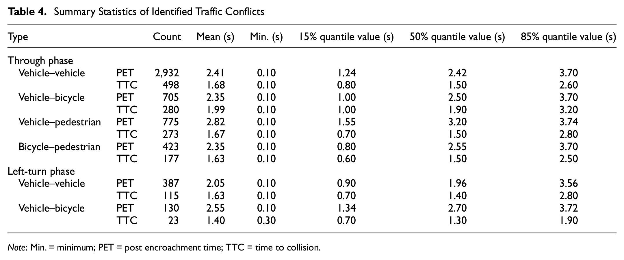
For the collected 10 h of LiDAR point data, a total of 5,352 traffic conflicts were identified by PET ≤ 4 s and a total of 1,366 traffic conflicts were identified by TTC ≤ 4 s. The greater number of conflicts identified by PET than by TTC is because most of the involved road users with overlapped trajectories were not on the collision course. The summary statistics of the collected traffic conflicts are shown in Table 4.

Table 4.

Summary Statistics of Identified Traffic Conflicts

Type		Count	Mean (s)	Min. (s)	15% quantile value (s)	50% quantile value (s)	85% quantile value (s)
Through phase
Vehicle–vehicle	PET	2,932	2.41	0.10	1.24	2.42	3.70
Vehicle–vehicle	TTC	498	1.68	0.10	0.80	1.50	2.60
Vehicle–bicycle	PET	705	2.35	0.10	1.00	2.50	3.70
Vehicle–bicycle	TTC	280	1.99	0.10	1.00	1.90	3.20
Vehicle–pedestrian	PET	775	2.82	0.10	1.55	3.20	3.74
Vehicle–pedestrian	TTC	273	1.67	0.10	0.70	1.50	2.80
Bicycle–pedestrian	PET	423	2.35	0.10	0.80	2.55	3.70
Bicycle–pedestrian	TTC	177	1.63	0.10	0.60	1.50	2.50
Left-turn phase
Vehicle–vehicle	PET	387	2.05	0.10	0.90	1.96	3.56
Vehicle–vehicle	TTC	115	1.63	0.10	0.70	1.40	2.80
Vehicle–bicycle	PET	130	2.55	0.10	1.34	2.70	3.72
Vehicle–bicycle	TTC	23	1.40	0.30	0.70	1.30	1.90

Note: Min. = minimum; PET = post encroachment time; TTC = time to collision.

It can be found from Table 4 that conflicts are more likely to occur during the through phase, and the majority of them are vehicle–vehicle conflicts. The main reason is the high volume of through vehicles. Through vehicles running on the right-most lane of the exit approach more likely to interact with the right-turn vehicles. In contrast, the left-turn vehicles usually take the left-most lane or the middle lane of the exit approach, and they have few chances to interact with the right-turn vehicles that usually run on the right-most lane. The conflicts between right-turn vehicles and vulnerable road users (i.e., bicycles and pedestrians) during the through phase are also an issue. These conflicts account for 30.6% and 45.0% of the total for PET and TTC, respectively. Although pedestrians have priority during the through phase (i.e., green light for through pedestrians), unyielding behavior of right-turn vehicles is common in China ( 34 ).

Conclusion

This study aims to identify different types of traffic conflict at signalized intersections, based on LiDAR data. Raw LiDAR point clouds were firstly processed by SDK to obtain original trajectories of different road users, and then methods were developed to handle the issues of trajectory discontinuity, type identification error, and same object with different trajectories. With the processed data, a procedure with three steps was proposed to calculate conflict indicators of TTC and PET; the steps were bounding box-related data calculation, potential conflict identification, and conflict indicator calculation. The developed methods were applied to LiDAR data points collected from a signalized intersection in Harbin, China, with a total duration of 10 h. Three types of conflict were considered: conflicts between right-turn vehicles and through vehicles, conflicts between right-turn vehicles and left-turn vehicles, and conflicts between right-turn vehicles and pedestrians. The automatically identified conflicts were compared with the manually identified ones, and the results show that the automatic method performs well, with accuracy in general over 90%.

In conclusion, this study showed the capability of using LiDAR data for efficient and accurate multi-type traffic conflict identification. However, it is more of a fundamental work and a first step for conflict-based road safety analysis. On the one hand, future work is needed to further improve the accuracy of the identified conflicts, and this could be done by improving the bounding boxes of road users and better handling the occlusion between road users. On the other hand, one continuation of this work is to embed the proposed LiDAR-based conflict identification method into the real-time crash prediction framework developed in Zheng and Sayed ( 3 ). With more efficient identified traffic conflicts, the timeliness of real-time prediction would be significantly improved.

Footnotes

Author Contributions

The authors confirm contribution to the paper as follows: study conception and design: L. Zheng; data collection: S. Ma; analysis and interpretation of results: L. Zheng, S. Ma, S. Fan, H. Jiao; draft manuscript preparation: S. Fan, H. Jiao. All authors reviewed the results and approved the final version of the manuscript.

Declaration of Conflicting Interests

The author(s) declared no potential conflicts of interest with respect to the research, authorship, and/or publication of this article.

Funding

The author(s) disclosed receipt of the following financial support for the research, authorship, and/or publication of this article: The support from the National Natural Science Foundation of China (Grant No. 52072097), the Science and Technology Project of Heilongjiang Province (Grant No. 2022ZXJ02A02) and the Heilongjiang Provincial Natural Science Foundation (Grant No. LH2019E052) are acknowledged.

ORCID iD

Lai Zheng

References

Wei

Zheng

Essa

Cycle-Level Traffic Conflict Prediction at Signalized Intersections With LiDAR Data and Bayesian Deep Learning. Accident Analysis and Prevention, Vol. 192, 2023, p. 107268.

Yuan

Abdel-Aty

Approach-Level Real-Time Crash Risk Analysis for Signalized Intersections. Accident Analysis and Prevention, Vol. 119, 2018, pp. 274–289.

Zheng

Sayed

A Novel Approach for Real Time Crash Prediction at Signalized Intersections. Transportation Research Part C: Emerging Technologies, Vol. 117, 2020, p. 102683.

FHWA Office of Safety. The National Intersection Safety Problem: Intersection Safety Issue Brief 2. FHWA-SA-10005. Department of Transportation, Washington, D.C., 2009.

Barua

Azad

Tay

Fatality Risks of Intersection Crashes in Rural Undivided Highways of Alberta, Canada. Transportation Research Record: Journal of the Transportation Research Board, 2010. 2148: 107–115.

Fernandes

Vehicle-Pedestrian Accidents at Signalized Intersections in Montreal. Dissertation. McGill University, Montreal, 2013.

Lord

Mannering

The Statistical Analysis of Crash-frequency Data: A Review and Assessment of Methodological Alternatives. Transportation Research Part A, Vol. 44, No. 5, 2010, pp. 291–305.

Zheng

Sayed

Mannering

Modeling Traffic Conflicts for Use in Road Safety Analysis: A Review of Analytic Methods and Future Directions. Analytic Methods in Accident Research, Vol. 29, 2021, p. 100142.

Amundsen

Hydén

(Eds.). Proc., 1st Workshop on Traffic Conflicts, Oslo, Norway, 1977.

10.

Zheng

Ismail

Meng

Traffic Conflict Techniques for Road Safety Analysis: Open Questions and Some Insights. Canadian Journal of Civil Engineering, Vol. 41, 2014, pp. 633–641.

11.

Mahmud

Ferreira

Hoque

Tavassoli

Application of Proximal Surrogate Indicators for Safety Evaluation: A Review of Recent Developments and Research Needs. IATSS Research, Vol. 41, 2017, pp. 153–163.

12.

Guido

Saccomanno

Vitale

Astarita

Festa

Comparing Safety Performance Measures Obtained From Video Capture Data. Journal of Transportation Engineering, Vol. 137, No. 7, 2011, pp. 481–491.

13.

Min

Kim

Cho

Development of an Automatic Traffic Conflict Detection System Based on Image Tracking Technology. Transportation Research Record: Journal of the Transportation Research Board, 2009. 2129: 45–54.

14.

T-Analyst. Software for Semi-Automated Video Processing. 2016. www.tft.lth.se/software.

15.

Ismail

Sayed

Saunier

Lim

Automated Analysis of Pedestrian-Vehicle Conflicts Using Video Data. Transportation Research Record: Journal of the Transportation Research Board, 2009. 2140: 44–54.

16.

Ismail

Sayed

Saunier

Automated Analysis of Pedestrian Vehicle Conflicts: Context for Before-and-after Studies. Transportation Research Record: Journal of the Transportation Research Board, 2010. 2198: 52–64.

17.

Xie

Ozbay

Yang

Mining Automatically Extracted Vehicle Trajectory Data for Proactive Safety Analytics. Transportation Research Part C: Emerging Technologies, Vol. 106, 2019, pp. 61–72.

18.

Shi

Zhao

Yao

Hale

Video-Based Trajectory Extraction With Deep Learning for High-Granularity Highway Simulation (HIGH-SIM). Communications in Transportation Research, Vol. 1, 2021, p. 100014.

19.

Swargiary

Kadali

A Study on Meta-Analysis Approach for Pedestrian-Vehicle Interaction Using LiDAR. Transportation Engineering, Vol. 13, 2023, p. 100191.

20.

Zhang

Bhattarai

Chen

Liu

Vehicle Trajectory Tracking Using Adaptive Kalman Filter From Roadside Lidar. Journal of Transportation Engineering Part A-Systems, Vol. 149, 2023, p. e04023043.

21.

Zhao

J. X.

J. Q.

Zheng

Y. C.

Liu

Trajectory Tracking and Prediction of Pedestrian’s Crossing Intention Using Roadside LiDAR. IET Intelligent Transport Systems, Vol. 13, 2019, pp. 789–795.

22.

Tarko

Ariyur

Romero

Bandaru

Liu

Stationary LiDAR for Traffic and Safety Applications–Vehicles Interpretation and Tracking. Project No. 134PY2.1. U.S. Department of Transportation, Washington, D.C., 2014.

23.

Zheng

Tian

A Novel Method of Vehicle-Pedestrian Near-Crash Identification With Roadside LiDAR Data. Accident Analysis and Prevention, Vol. 121, 2018, pp. 238–249.

24.

Zhang

Sun

An Improved Vehicle-Pedestrian Near-Crash Identification Method With a Roadside LiDAR Sensor. Journal of Safety Research, Vol. 73, 2020, pp. 211–224.

25.

Sun

Zhang

Yue

Automatic Vehicle-Pedestrian Conflict Identification With Trajectories of Road Users Extracted from Roadside LiDAR Sensors Using a Rule-based Method. IEEE ACCESS, Vol. 7, 2019, pp. 161594–161606.

26.

Vasudevan

Agarwala

Tiwari

LiDAR-Based Vehicle-Pedestrian Interaction Study on Midblock Crossing Using Trajectory-Based Modified Post-Encroachment Time. Transportation Research Record: Journal of the Transportation Research Board, 2022. 2676: 837–847.

27.

Bhattarai

Zhang

Liu

Pakzad

Proactive Safety Analysis Using Roadside LiDAR Based Vehicle Trajectory Data: A Study of Rear-End Crashes. Transportation Research Record: Journal of the Transportation Research Board, 2023. 2678: 772–785.

28.

Zhao

Liu

Zheng

Detection and Tracking of Pedestrians and Vehicles Using Roadside LiDAR Sensors. Transportation Research Part C: Emerging Technologies, Vol. 100, 2019, pp. 68–87.

29.

Zhang

Xiao

Coifman

Mills

Vehicle Tracking and Speed Estimation From Roadside LiDAR. IEEE Journal of Selected Topics in Applied Earth Observations and Remote Sensing, Vol. 13, 2020, pp. 5597–5608.

30.

Cui

Wang

Lane Change Identification and Prediction With Roadside LiDAR Data. Optics and Laser Technology, Vol. 123, 2020, p. 105934.

31.

Cao

Wang

Liu

Trajectory-Based Method for Dividing Lanes of Vehicle Trajectories Collected by Roadside LiDAR. Transportation Research Record: Journal of the Transportation Research Board, 2023. 2678: 816–828. https://doi.org/10.1177/03611981231182987

32.

Hayward

Near Misses as a Measure of Safety at Urban Intersections. Dissertation. The Pennsylvania State University, 1971.

33.

Cooper

Experience With Traffic Conflicts in Canada With Emphasis on Post Encroachment Time Techniques. International Calibration Study of Traffic Conflicts, Copenhagen NATA ASI Series F5, 1984, pp. 75–96.

34.

Wang

Sun

Evaluation of Pedestrian Safety at Intersections: A Theoretical Framework Based on Pedestrian-Vehicle Interaction Patterns. Accident Analysis and Prevention, Vol. 96, 2016, pp. 118–129.