Hybrid Transfer Learning and Support Vector Machine Models for Asphalt Pavement Distress Classification

Image Classification Versus Image Detection

In the context of CNNs, image detection and image classification refer to two different tasks that can be performed on input images. It is thus important to explicitly distinguish between the two to prevent confusion and to facilitate appropriate evaluation. Image classification is the task of assigning a single label or category to an input image. Image detection, on the other hand, is the task of identifying the presence and location of objects of interest in an input image. The current study is limited to image classification of eight selected asphalt pavement distresses as the authors believe the process of assigning labels to an entire image is the first important step in both image classification and object detection. Once a model(s) has been developed for the classification task, object detection can be easily performed by passing features extracted from the classification stage as inputs for the detection stage.

Classification for Asphalt Pavement Distress

In most cases, road surface conditions are typically assessed visually, either manually or automatically using specially equipped vehicles. While some data collection aspects have been automated, classifying pavement distress remains a tedious and subjective task. Existing methods are often semi-automated, requiring further analysis by experienced technicians or expensive proprietary systems. Additionally, reported costs for some automated systems are high, averaging about $1.2m to acquire a unit and about $70k/year to operate (Vavrik et al. [ 4 ]), making them less accessible. Consequently, many agencies still prefer manual inspection, considering it more convenient ( 5 ) or only surveying intermittently. Continuous monitoring for distress initiation and propagation is essential for cost-effective maintenance, which existing systems struggle to achieve. The challenge of replicating the expertise of trained technicians, reducing survey costs, and the need for continuous monitoring could be addressed by leveraging DL techniques, particularly hybrid TL and SVMs.

Transfer Learning for Asphalt Pavement Distresses

There have been several studies that have explored the use of TL for the classification of asphalt pavement distresses in the attempt to automate asphalt pavement distress inspections. The studies have generally used DL models such as CNNs and TL techniques such as fine-tuning and feature extraction. Most of these previous studies have focused on the development of TL classification networks based entirely on single DL models such as Inception ( 6 – 27 ). Overall, these studies demonstrate the effectiveness of TL for improving the accuracy of DL models for asphalt distress classification. However, the accuracy of TL models can depend on various factors, such as the quality and size of the labeled data set, the choice of pretrained model, and the specific type of asphalt distress being classified. Few studies have attempted hybrid models involving multiple machine learning techniques. A key focus of the current study is to fill the gap related to the choice of pretrained models for TL since previous studies have shown significant differences in the performance of various pretrained DL models ( 9 ).

Apeagyei et al. ( 9 ) evaluated various state-of-the-art pretrained DCNNs for developing pavement distress classification models using TL approaches. Results indicated significant differences in the performance of selected pretrained networks in relation to accuracy. They identified the need for future studies to focus on image quality and quantity, exploration of hyperparameter variability, and consideration of synergistic effects from combining multiple DCNNs for improved predictive performance.

Support Vector Machine (SVM)

SVM is a supervised machine learning procedure that is frequently employed for tasks involving classification and regression. While DL approaches have gained significant attention in recent years, SVMs were popular for image classification tasks before the rise of DL architectures. There have been many studies that have used SVMs for the detection of highway distresses. For example, Lin and Liu ( 13 ) investigated the possibility of detecting potholes on roads from digital images using SVMs. The researchers extracted color and texture features from digital road images and used an SVM classifier to distinguish between potholes and non-pothole areas. The SVM model showed promising results in accurately identifying potholes from the road images. Others include Gavilán et al. ( 14 ) who used multiclass SVMs to classify 10 pavement surface types so that features could be manually selected for the subsequent road distress detection module. The authors identified the need for a more sophisticated and automated approach to feature extraction.

Carvalhido et al. ( 15 ) proposed a crack classification technique using SVMs. The approach required three different preprocessing configurations to smoothe the texture and enhance potential cracks in images. The authors suggested the need for additional preprocessing techniques, such as median and morphological filters to improve the robustness of their models. The study was limited to cracks whereas a typical highway will involve multiple distresses.

Prasanna et al. ( 16 ) proposed a histogram-based classification algorithm and applied it together with SVM to detect cracks on the concrete deck surface; the results on bridge data highlighted the need to improve the accuracy of practical predictions.

Gavilán et al. ( 14 ) proposed an automated crack detection system to distinguish between cracked and non-cracked areas on up to 10 different types of pavement using a linear SVM-based classifier ensemble. The Gray-Level Co-Occurrence Matrix (GLCM), Maximally Stable Extremal Regions (MSER) and Local Binary Patterns (LBP) were used to obtain the components of the feature vector. The authors recommended future studies that involve new performance indexes to differentiate between diverse types of crack such as longitudinal, transverse, and alligator cracking.

Ai et al. ( 17 ) proposed an SVM-based method to calculate the probability maps using the information of multi-scale neighborhoods to develop a fused map, which can detect cracks with accuracy higher than any of the original probability maps. The models were evaluated using performance metrics including precision, recall, F1-score, and receiver operating characteristics. The study was limited to the pixel level pavement crack detection problem at the expense of all other common pavement distresses. Furthermore, feature extraction was obtained in part using a probabilistic generative model–based method designed to calculate the probability of a crack for each pixel.

Hadjidemetriou et al. ( 18 ) proposed an automated vision-based method for detecting and quantifying pavement patches, which are vital for evaluating and rating pavement surfaces. The proposed system uses video frames captured from either a smartphone or an external camera positioned inside or outside a moving passenger vehicle. SVM classification is employed on feature vectors extracted from the images, using two texture descriptors and the histogram of nonoverlapped square blocks. These feature vectors enable the characterization of image blocks as either patch or non-patch areas. The output of the system provides block-based and image-based classifications. The method demonstrated a detection accuracy of 82.5% for image-based classification.

Hoang and Nguyen ( 19 ) compared classification algorithms using machine learning and image processing techniques such as steerable filters, the projective integral of the image, and an enhanced method for image thresholding. Feature extraction was based on image processing and texture computation. The results showed that SVM had the highest level of classification accuracy at 87.50%, followed by artificial neural networks (ANNs) at 84.25%, and random forest (RF) at 70%.

Sari et al. ( 20 ) examined an automation method of classification and segmentation of asphalt pavement cracks to classify asphalt pavement cracks using the SVM algorithm and segmentation method of the OTSU algorithm. The approach involved classification of distress data into two groups: with crack and no crack. The models were evaluated using multiple performance metrics including accuracy, precision, recall, area under receiver operating characteristic (ROC) curve (AUC), and ANOVA statistical test. The authors suggested that the SVM algorithm combined with OTSU segmentation and GLCM feature extraction could be used for the classification of asphalt pavement cracks.

The review of existing studies shows that the majority of TL based studies on pavement distress classification were limited to the evaluation of one or two existing models. Additionally, some existing models do not transfer accurately when applied to new learning so the use of one or two models for training is a major limitation for the pavement distress identification area. The number and definition of distress classes varied widely from two to nine. The studies reviewed demonstrate TL’s effectiveness in improving DL models’ accuracy for pavement distress classification. However, the need for future studies to focus on the choice of pretrained models for TL, considering significant differences in performance among various DCNN models. Furthermore, exploration of image quality and quantity, investigation of hyperparameter variability, and consideration of synergistic effects from combining multiple distress classification models require further investigation. Reviews of multiple studies using SVM for highway distress detection show the potential of the technique. However, none of the studies reviewed explored the application of hybrid SVM and TL to address issues such as limitation of training, class imbalance, automated feature extraction, accuracy, and variability in performance of pretrained DCNN models. Even though some of the selected models have been used in previous TL applications for pavement distress identification, very few, if any, have used the more robust graphical performance measures such as ROC, AUC, and t-SNE.

The paper’s significance lies in its development of a hybrid model that effectively addresses challenges in automating pavement distress evaluation, using DL for feature extraction and SVMs for classification, thereby improving accuracy and offering a potential solution to reduce costs and enhance safety in pavement management.

Data Collection

The data collection and preprocessing step consisted of assembling a data store of distress images with category labels. The eight distress labels used in this study have been assigned by taking the names of the folders that contain the image files. The images were automatically resized to the correct image size based on the pretrained model.

Around 400 pictures of asphalt pavement distresses were obtained from various publicly accessible sources, which included Google Street, a commonly used method in this field. The 400 images were manually categorized into eight class labels which are block cracking, distress free, fatigue cracking, longitudinal cracking, patching, pothole, rutting, and transverse cracking by trained technicians. To process each classified image for each network type, user-defined functions were used for preprocessing into the required input size. The images were then randomly divided into training (85%) and validation (15%) groups. Samples of the images used and the distribution of images in each distress class are presented in Figure 1. As can be seen in Figure 1, the distribution of images is imbalanced, with the number of images per class ranging between 30 and 60. It is common to have such imbalanced or skewed class distributions with most pavement distress data sets given the climatic factors, traffic loading, and functional classification of the road. Additional distress images were obtained from an actual project located in southern Africa for verification of the most promising models to verify the models’ performance and assess their generalization ability.

OPEN IN VIEWER

Figure 1.

Sample images: (a) used for training and validating the networks; (b) their distribution into the eight distress classes.

Class imbalance is a fundamental problem in DL classification problems, where some classes have significantly fewer samples than others. In such cases, a DL trained on an imbalanced data set may be biased toward the majority class and have inferior performance on the minority class. The imbalanced class distribution can lead to overfitting of the model to the majority class, which can result in poor generalization to new and unseen data. Furthermore, the standard performance metrics, such as accuracy, precision, and recall, which are commonly used to evaluate the model’s performance, may not provide an accurate representation of the model’s performance in such scenarios. To overcome this problem, the technique of undersampling the majority class was found to lead to better model performance than either oversampling or generative adversarial networks (GAN)–generated synthetic images. Thus, all the models were developed by randomly undersampling the majority classes so that each class had the same number of images equal to the number of images in the minority class (i.e., 31 images).

Pretrained Deep Learning Models

Eight pretrained DL models were selected including Alexnet, Densenet, Googlenet, Mobilenet, Resnet50, Squeezenet, VGG19, and Xception. The selected models have been pretrained on the large-scale ImageNet data set for image classification. ImageNet is a data set that contains millions of labeled images, and it has been widely used as a benchmark for testing and comparing the performance of DL models for image classification. The eight models were chosen because they all achieved state-of-the-art performance on various image classification tasks. Further details of the selected DL models including a description of model performance on asphalt pavement distress classification can be found in Apeagyei et al. ( 9 ).

The feature extraction step involved using the pretrained model to extract features from the input images. This step also involves removing the classification layers of the pretrained model and using the remaining layers to extract features from the images. Following the feature extraction step, training of the selected pretrained models followed. This step involved tuning model hyperparameters to optimize performance and comprised of using the stochastic gradient descent with momentum (SGDM) as the optimizer, selecting the initial learning rate, specifying minibatch size depending on model size, and setting maximum epochs of 12 to optimize training time and accuracy. It should be noted that the selection of the aforementioned parameters was based on an extensive trial and error approach as well as the authors’ experience in the field.

The pretrained models were fine-tuned by unfreezing some of their layers and retraining them on the new data set. This step involves selecting the layers to be unfrozen and adjusting the learning rate to avoid overfitting. In this study, the models were fine-tuned by replacing the last three layers, which included the fully connected layer, the softmax layer, and the classification layer. The rest of the layers were kept frozen, which is a common method used by previous researchers to achieve the best predictive accuracy for their models. However, the number of layers to freeze or train can vary among different investigators. Some studies have replaced more layers than the three used in this study, but it should be noted that this does not always result in better models. The ultimate goal for all researchers is to achieve the best possible accuracy in their models.

For the current study, three strategies were evaluated: the traditional single transfer learning-based DL models (TLDL), hybrid DL+SVM, and hybrid TLDL+SVM. A schematic of the approach is depicted in Figure 2. A brief description of each strategy is discussed next.

OPEN IN VIEWER

Figure 2.

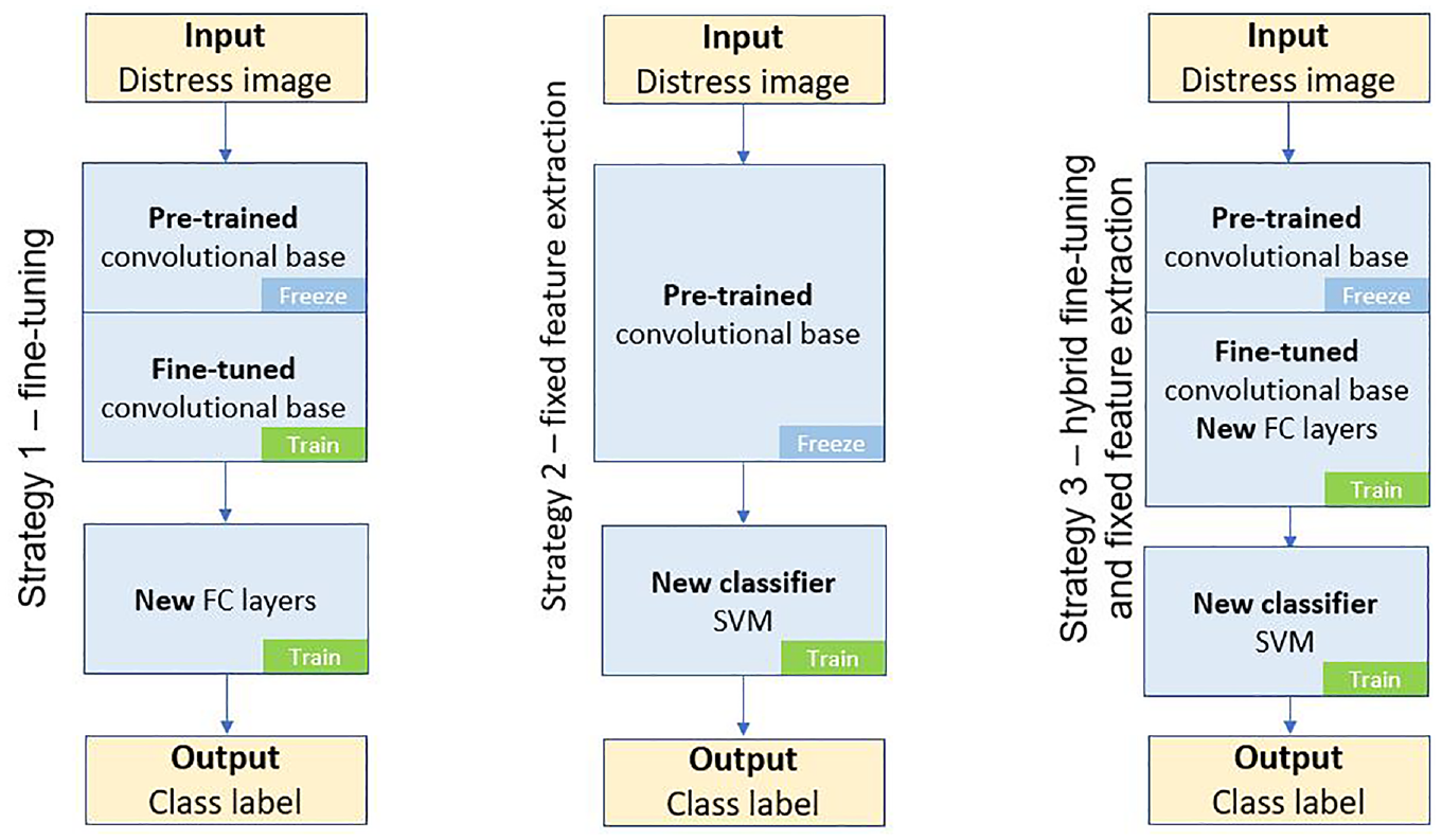
Strategies for developing and evaluating hybrid DL and SVM models for asphalt pavement distress classification.

Evaluation of Retrained Models

The prediction performance of each retrained DCNN hybrid model was evaluated by comparing confusion matrix statistics and accuracy measures such as precision, overall accuracy, and recall, which have commonly been used to assess how well TL-based DCNNs performed by most previous investigators. In addition, combined measures such as F1-score and graphical measures including ROC, AUC, t-SNE, and so forth., that are more robust against class imbalance and overfitting were used.

Confusion Matrix

The predictive performance of a DL model can be visualized using a confusion matrix (CM), which presents the results in a tabular format. Each element of the CM represents the number of predictions made by the network and whether they were classified correctly or incorrectly. Evaluating the diagonal entries of the CM is a common method to assess the success of a DCNN classifier. To correctly interpret the CM results, it is important to consider some fundamental concepts, which are further explained by Düntsch and Gediga ( 21 ). In a two-class classification problem, where typically a positive and a negative class are involved, four metrics are commonly used. These metrics include true positives (t_p), false positives (f_p), true negatives (t_n), and false negatives (f_n).

These metrics can be used to estimate various key performance measures such as accuracy, F1-score, precision, recall, and specificity (Equations 1–5). Others include ROC curve, and area under the curve (AUC) for a given network. The overall accuracy is evaluated using the F1-score, which is the harmonic mean of recall and precision. The F1-score balances the trade-off between precision and recall. A value of 0 for the F1-score indicates that either the precision or the recall is 0.

Accuracy = t p + t n t p + t n + f p + f n

(1)

Precision = t p t p + f p

(2)

Recall = t p t p + f n

(3)

Specificity = t n t n + f p

(4)

F 1 − score = 2 t p 2 t p + f p + f n

(5)

Accuracy

The performance of the trained networks using the three strategies was evaluated using multiple performance measures including overall accuracy and F1-score (Figure 3) obtained from confusion matrices. The results obtained highlight the impact of the training strategy on the performance of the models. It is evident from Figure 3 that the choice of strategy significantly influenced the overall performance, with the models trained using Strategy 2 demonstrating comparatively poorer results. Conversely, all models exhibited strong performance under Strategy 3. A comprehensive analysis of the outcomes indicates that there exist statistically significant differences in performance between Strategy 1 and Strategy 2 (p-value = 0.001). Furthermore, the results unequivocally indicate that Strategy 3 outperforms both Strategy 1 and Strategy 2 by a significant margin (p-value < 0.000011). Specifically, the accuracy of models trained under Strategy 3 was notably superior to the accuracy achieved by the other two models. This finding aligns with our expectations, as it substantiates the superior capabilities of the models trained using the hybrid DL and SVM models. The detailed performance metrics of the models are presented in Figure 3 where the average performance for the three strategies were 0.6945 ± 0.066, 0.5486 ± 0.069, and 0.9383 ± 0.019, respectively for Strategy 1, Strategy 2, and Strategy 3.

OPEN IN VIEWER

Figure 3.

Evaluation of pretrained DCNN models’ performance (F1) with different training strategies.

Computational Time and Model Complexity

Figure 4 shows a comparison of the three strategies for training times and model complexity (assumed to be related to the size on file of each trained model). In the presented bubble plot depicting the performance of three strategies, the y-axis spans from 0 to 100%, representing the accuracy of each model, while the x-axis extends logarithmically from 0 to 1,460. The bubble sizes correspond to the respective sizes of the models on disk, providing a visual representation of their complexities. Strategy 1 models are centered on the graph, showcasing a balanced trade-off between model size, training time, and accuracy. Strategy 2 models are positioned near the left-middle corner of the plot, indicating a modest model size, moderate accuracy, and shorter training time. In contrast, Strategy 3 models are situated near the upper right corner, signifying superior accuracy and a larger size on disk compared with the other models. The distinct locations of the three models on the plot offer a clear illustration of their trade-offs between accuracy and storage efficiency, with Strategy 3 models emerging as the top performers in predictive accuracy. The training times for Strategy 2 and Strategy 3 can be considered as comparable, with the difference in most cases differing by a few dozens of seconds.

OPEN IN VIEWER

Figure 4.

Comparison of the training speeds versus module complexity (size on disk) for eight pretrained SVM-DCNNs hybrid asphalt pavement distress classification models.

Robustness of Hybrid Models

As previously discussed, during training, distress images were randomly sampled for both training and testing. This necessary step naturally introduces randomness into the development of the models. Thus, it was deemed necessary to assess the robustness and repeatability of the SVM hybrid models’ performance. Experiments were conducted that involved 10 separate runs of model training. For each experimental run, the F1 parameter was recorded. Figure 5 provides a summary of the results in the form of box-and-whisker plots. The comparative analysis of the experiments revealed interesting insights into their performance. It can be seen from Figure 5 that the performance of the models varied widely. For instance, considering Figure 5a, Xception achieved the highest median F1 score of 0.67, followed closely by Alexnet (0.63) and Squeezenet (0.61). Large variability in F1 was observed across all the modules with some models exhibiting data that allows them to be considered outliers. None of the literature reviewed reported this variability in training data as many authors only reported data for the best modules. Thus, this study contributes to our understanding of this important phenomenon. A classifier with an average F1 score of about 0.51 can be considered to be performing slightly better than random guessing, especially if there are eight different classes in the data set, as is the case in this study. If a classifier’s accuracy is consistently around 0.51, it suggests that the model is not able to capture the underlying patterns or features that differentiate the classes effectively. In other words, the classifier is making incorrect predictions more often than correct ones. While it may not be accurate to describe the classifier as a random number generator, as it still shows some capability to differentiate between classes, it is clear that there is room for improvement in its performance. Overall, the performance of Strategy 2 was only slightly better than a random model as the average F1-score for all pretrained models combined was slightly more than 0.51.

OPEN IN VIEWER

Figure 5.

Quantifying model reliability and stability: F1-score distribution across 10 repeat runs; (a) Strategy 1, TLDL; (b) Strategy 2, DL-SVM; (c) Strategy 3, TLDL-SVM.

For Strategy 3 (see Figure 5c), among the tested models, Xception consistently exhibited the highest median F1 score of 0.9633, closely followed by Densenet (0.9630) and Googlenet (0.9519). These models consistently demonstrated strong classification capabilities across multiple test runs, indicating their effectiveness in distinguishing different distress types in asphalt pavement. On the other hand, models such as Squeezenet (0.9056) and VGG19 (0.9023) achieved slightly lower average F1 scores, suggesting comparatively lesser performance in classifying pavement distresses. It is worth noting that while these models had relatively lower average F1 scores, they still showed acceptable performance levels. Furthermore, the standard deviations for all models were relatively low, indicating consistency in their performance across different test runs. This consistency implies that the Strategy 3 models’ classification performance is reliable and robust.

Receiver Operating Characteristic (ROC) Analysis

ROC analysis was used as an evaluation metric to assess the performance of the classification models and their ability to discriminate between the different classes of pavement distresses. In image classification tasks, a model predicts the probability or confidence of an image belonging to a certain class. The output of the model can be interpreted as a continuous score or a probability. To construct an ROC curve, the model’s output scores are used to calculate the TPR (recall) and the FPR (1 – specificity) at various classification thresholds. A classification threshold is applied to these scores to determine the predicted class labels. By varying the threshold, the trade-off between the TPR and the FPR can be adjusted. A lower threshold leads to more positive predictions, while a higher threshold results in fewer positive predictions. Based on the selected threshold, the model’s predictions are compared with the ground truth labels of the images. The TPR is the ratio of correctly predicted positive samples (e.g., images from the positive class) to the total number of positive samples. The FPR is the ratio of incorrectly predicted positive samples to the total number of negative samples (e.g., images from the negative class). On an ROC, the TPR is plotted on the ordinate, and the FPR is plotted on the abscissa. By varying the threshold and calculating the TPR and FPR at each point, multiple (TPR, FPR) pairs are obtained. Connecting these points creates the ROC curve. The ROC curve provides valuable insights into the trade-off between recall and specificity in the classification task. A classifier with a higher ROC curve, closer to the top-left corner, indicates better performance in distinguishing between classes (Figure 6). The ROC curve shows a solid circle symbol at the operating point of the model for each class. The dotted line on the graph represents a random model. A perfect model is indicated by TPR equal to 1 and FPR equal to 0. On the other hand, the worst model is represented by TPR equal to 0 and FPR equal to 1. In the legend, the class name and corresponding AUC value are provided for each curve. In Figure 6, we compare the ROC curves obtained from Strategy 2 and Strategy 3 when using the Mobilenet pretrained network. The ROC curves for Strategy 3 (hybrid TLDL+SVM) are plotted higher and closer to the top-left corner compared with Strategy 2, indicating superior performance. Moreover, Figure 6 shows that the AUC for Strategy 2 ranged from 0.6843 to 0.9824, while for Strategy 3 it ranged from 0.9757 to 1.0000. The ROC curve and its associated AUC demonstrate that the hybrid TLDL+SVM method possesses superior predictive capability in distinguishing distressed pavements across multiple classes. Similar findings were observed across all the other models analyzed. These results suggest that Strategy 3 consistently outperforms Strategy 2 when using the eight pretrained networks.

OPEN IN VIEWER

Figure 6.

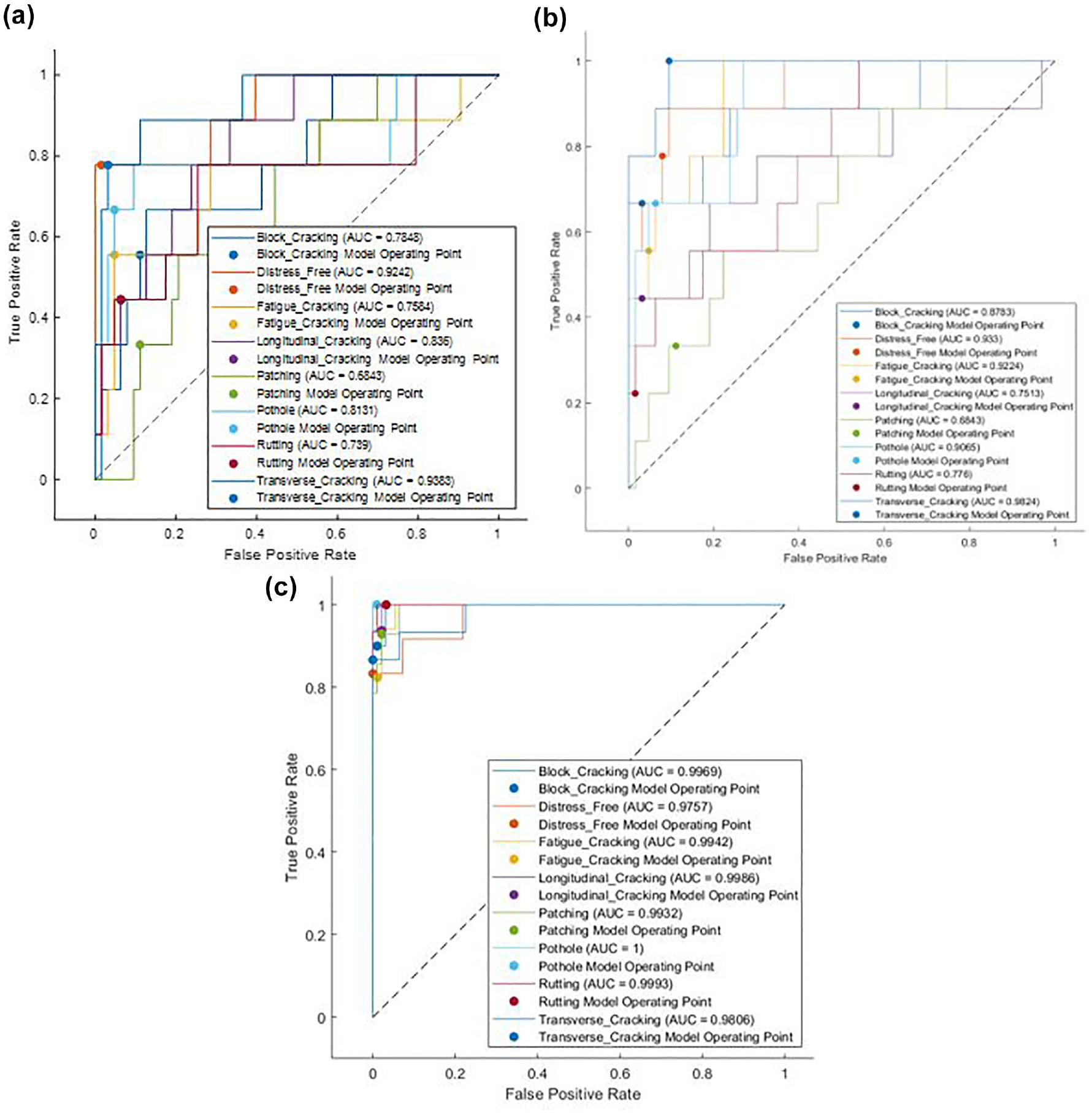
Comparison of ROC curves for hybrid SVM and DL pavement distress classification models; (a) Strategy 1; (b) Strategy 2; (c) Strategy 3.

The AUC is calculated as the integral of the ROC curve. It represents the overall performance of the classifier across all possible threshold values. An AUC value of 1 indicates a perfect classifier, while an AUC value of 0.5 suggests a random or no-discrimination classifier.

Comparing the Statistical Significance of the Performance of Hybrid TL and SVM Classifiers

The results obtained from our study demonstrate that employing transfer-learned models as feature extractors, combined with SVM as the classifier, yields superior performance (F1-score greater than 0.90, AUC greater than 0.98, and ROCs that plot in the top lefthand corner) regardless of the pretrained network used. To determine if significant differences exist among the different models developed under Strategy 3, we conducted the Kruskal–Wallis test followed by the Dunn’s test. The Kruskal–Wallis test is particularly valuable for analyzing data when the assumptions of parametric tests, such as normality and equality of variance, are not met or not known, especially in scenarios involving multiple groups. In Dunn’s test, the mean ranks are employed to assess the statistical significance of the differences between groups. A significant difference in mean ranks indicates that the groups are statistically distinguishable from each other, without providing information about the direction or magnitude of the difference. The results of the Dunn’s test conducted on the pairwise comparisons between the eight different network groups (Alexnet to Xception) showed that significant differences exist between certain pairs of groups. For example, Densenet versus Resnet50, Densenet versus Squeezenet, Densenet versus VGG19, Googlenet versus Squeezenet, Googlenet versus VGG19, Googlenet versus Xception, Resnet50 versus Xception, Squeezenet versus Xception, and VGG19 versus Xception show p-values less than 0.05, suggesting statistically significant differences. The Dunn’s test results reveal both significant and non-significant differences between the groups, providing valuable insights into the comparative performance of the various groups under investigation. It can be inferred from the results that even though all Strategy 3 models performed very well, models based on the three pretrained networks, Densenet, Googlenet, and Xception, are outstanding as compared with previous studies ( 8 – 27 ).

Extracted Features

To gain insight into the distribution, relationships, and separability of the extracted features across the different classes of images, the dimensionality reduction technique known as t-distributed stochastic neighbor embedding (t-SNE) was applied to the extracted features comprising eight classes and 255 columns of data. The results of the t-SNE visualization are depicted in Figure 7. When conducting a t-SNE visualization of extracted features from a DL model, if the classes plot on separate parts of the figure with no overlaps, similar to Figure 7, it suggests that the extracted features have distinct and well-separated representations for each class. This separation indicates that the DCNN has successfully learned discriminative features that can effectively differentiate between the different classes. In other words, the t-SNE visualization shows that the DL network has been able to capture meaningful patterns and structures in the data, resulting in a clear separation of the classes in the feature space. This is desirable as it implies that the DL network has learned to encode relevant information specific to each class, enabling accurate classification or recognition of the different categories. The absence of overlaps between the classes in the t-SNE plot indicates that the extracted features have high intra-class similarity and low inter-class similarity. It suggests that instances belonging to the same class are closer to each other in the feature space, while instances from different classes are farther apart. This separation can be seen as an indication of the effectiveness of the DCNN in capturing the distinctive characteristics and discriminative information associated with each class. The results justify the two-step approach proposed in this study.

OPEN IN VIEWER

Figure 7.

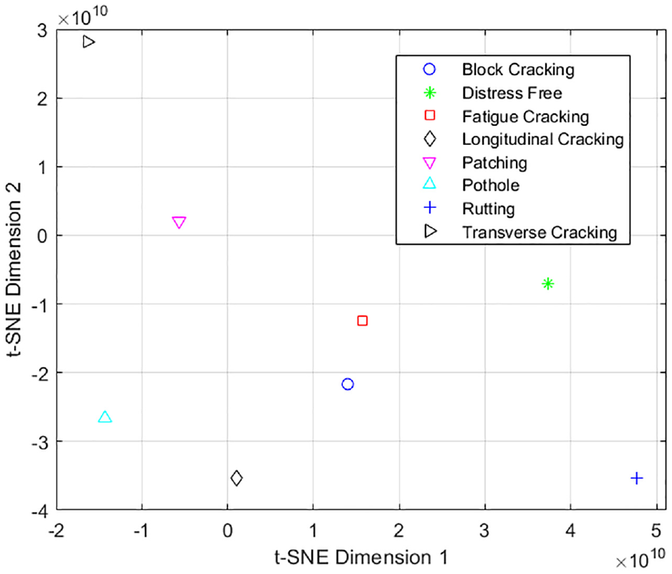
Sample t-SNE visualization of extracted features from retrained Mobilenet for Strategy 3. The symbols represent the eight distress classes arranged in alphabetical order from block cracking to pothole.

Verification of Models Based on the Most Promising Strategies

In addition to the training and validation process previously discussed in the development of the models, it is also common to have a final testing set that remains completely separate from both the training and validation sets. This testing set is designed to provide an unbiased assessment of the model’s performance after the entire development process. It helps evaluate how well the model generalizes to completely new data and provides a more reliable estimate of its real-world performance. This step thus serves to verify the model’s performance and assess its generalization ability. Therefore, as a further check on the performance and generalization ability of the models developed using the promising approach (Strategy 1 and Strategy 3), a new set of distress images which were not part of the data set used in the training and validation of the models was acquired from a project completed in southern Africa by one of the co-authors of the current paper ( 27 ). That project involved detailed forensic investigation to determine the causes of premature failure of asphalt concrete in Tanzania and contained a large data set of distress images which provided an ideal opportunity for verifying the performance accuracy of the models developed in this.

Figures 8 to 11 show the results of analysis based on Strategy 3; similar results were obtained for Strategy 1. Also shown in Figures 8 to 11 are the level of confidence attached by the model to the classification of each image. For example, the model assigned 100% confidence to the image in Figure 11, classifying it as patching. In Figure 8, the model was conflicted assigning a label of transverse cracking to the image with about 58% confidence but at the same time providing evidence that the distress could be longitudinal cracking. It should be noted that this is a common problem even with human experts and in line with previous studies ( 20 – 26 ).

OPEN IN VIEWER

Figure 8.

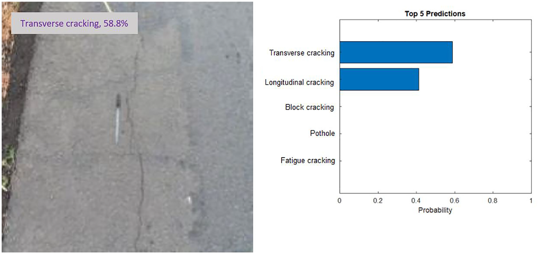
Verification of most promising models based on Strategy 3 for transverse cracking.

OPEN IN VIEWER

Figure 9.

Verification of most promising models based on Strategy 3 for rutting.

OPEN IN VIEWER

Figure 10.

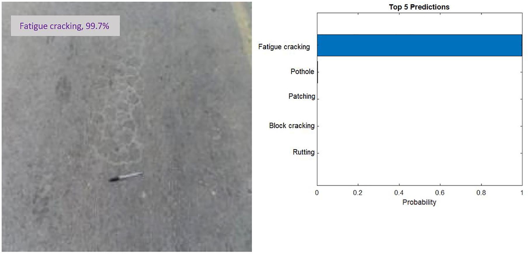
Verification of most promising models based on Strategy 3 for fatigue cracking.

OPEN IN VIEWER

Figure 11.

Verification of most promising models based on Strategy 3 for patching.