
Abstract
Accurate traffic flow data are important for congestion identification and real-time traffic control. Raw traffic flow data may be disturbed by different noises during the acquisition process, which leads to the degradation of model prediction performance. To address this problems, this paper proposes a data denoising method based on the improved complete ensemble empirical mode decomposition with adaptive noise (ICEEMDAN) combined with wavelet threshold denoising (WTD) to suppress potential outliers in the data, and then introduces functional principal component analysis to accomplish the traffic forecasting task. We use the proposed framework for real traffic flow prediction and validate the prediction performance of the proposed framework using root mean square error and mean absolute error. In the prediction performance comparison, five denoising methods are considered: empirical mode decomposition (EMD), ensemble empirical mode decomposition, complete ensemble empirical mode decomposition with adaptive noise, ICEEMDAN, and WTD. The prediction results show that the model combined with the denoising method outperforms the model without the denoising method. ICEEMDAN combined with WTD’s denoising method improves prediction performance more than other methods. Furthermore, the WTD method with dmey type achieves higher accuracy than other types.
Keywords
In the development of intelligent transportation systems, traffic flow prediction is a crucial issue, important for improving traffic safety and travel efficiency and for relieving traffic congestion ( 1 , 2 ). Accurate and timely traffic flow prediction can provide traffic management departments with appropriate traffic management control plans, and provide travelers with accurate and reliable travel routes, thus improving the efficiency of travel, which can only be achieved through the development of prediction models ( 3 ). However, given the complex external environment of the traffic system, the raw traffic data collected by the detector may be disturbed by some unobservable factors. These disturbances, which we call noise, can lead to a reduction in the predictive performance of the model ( 4 – 10 ). Therefore, denoising the traffic flow data during data processing is crucial. It was found that the prediction performance of the model incorporating the denoising technique was significantly better than that of the model without denoising treatment ( 11 ). Currently, widely used denoising methods include the Kalman filter, empirical modal decomposition, wavelet analysis, among others.
Numerous studies have employed such methods to enhance the quality of traffic flow data. For example, Tan et al. ( 12 ) used wavelet transform to reduce the noise of the original traffic data. Jiang and Adeli ( 13 ) introduced an improved discrete wavelet packet transform to handle the implied noise in the original data and used the autocorrelation function to select the number of decomposition layers in the wavelet method. Xie et al. ( 14 ) combined two types of wavelet models with a Kalman filter for short-time traffic prediction and showed that the wavelet Kalman filter model exhibited higher performance by mitigating the effect of noise. Zhang et al. ( 15 ) proposed an improved Kalman filter by designing a cost function to retain the useful signal while reducing the noise. Cai et al. ( 16 ) proposed a maximum entropy derived Kalman filter for a traffic flow prediction task considering that real traffic flow data are not Gaussian distributed. Peng and Xiang ( 17 ) proposed a wavelet denoising and phase space reconstruction model for traffic data sets to predict non-smooth spatial trends. Empirical mode decomposition (EMD) can decompose any complex signal into simple components. Chen et al. ( 18 ) used a fusion data denoising scheme (including EMD and wavelet decomposition) to remove potential data outliers. In conclusion, numerous studies have shown that the decomposition algorithm and data denoising process can reduce the influence of noise on the prediction model, which is an effective means of improving the accuracy of traffic flow prediction. However, these current denoising methods also have some limitations. For example, the wavelet transform is sensitive to parameter selection and requires the selection of appropriate wavelet basis functions and decomposition levels. Improper selection may affect the denoising effect: the Kalman filter relies on accurate system and noise models; if the models are inaccurate, the denoising effect will suffer; EMD may have modal mixing in case of very strong noise or complex signals, affecting the denoising effect; the Butterworth filter may introduce phase distortion although it has good smoothing in the frequency domain. Also, it may not be suitable for real-time traffic applications because of filtering delays; moving average (MA) is sensitive to the window size, and improper window size can lead to excessive signal smoothing or incomplete noise removal.
While denoising methods are crucial for improving the quality of traffic flow data, it is equally important to focus on the prediction model itself. Currently, many scholars have proposed many models for the traffic flow prediction problem. Traffic prediction models and methods can be roughly divided into two categories: classical methods and deep learning methods. Classical methods include statistical methods and traditional machine learning methods. The statistical approach is to build a data-driven statistical model to make predictions. The most typical are autoregressive integrated moving average (ARIMA) ( 19 ) and vector autoregression (VAR) ( 20 ). However, these methods are only applicable to relatively small data sets, and their prediction accuracy is not high as the data set increases. With the rapid rise of machine learning methods, support vector regression (SVR) ( 21 ) and random forest regression (RFR) ( 22 ) have been proposed for traffic flow prediction problems. These methods have the ability to handle high-dimensional data and capture complex nonlinear relationships. Although these methods have proved to be effective and feasible in traffic flow prediction, they usually require higher computational load and storage pressure. This is not appropriate when many training samples are available. With the development of deep learning methods, artificial intelligence is gradually taking advantage of its strength in traffic flow prediction ( 23 ). The most representative deep learning methods are recurrent neural network (RNN) ( 24 , 25 ), long short-term memory (LSTM) ( 26 ) and gate recurrent unit (GRU) ( 27 ). Inspired by the successful application of convolutional neural networks (CNN) in computer vision, many scholars have used CNN widely to extract spatiotemporal features of traffic flow. Zhang et al. ( 28 ) established a CNN-based deep learning framework to predict traffic flow and effectively extract spatiotemporal features. Given the weak ability to extract features from a single model structure, Zheng et al. ( 29 ) proposed convolution LSTM (ConvLSTM) to realize common spatiotemporal feature extraction. To improve the performance of traffic flow prediction models for road networks, graph convolution network (GCN) is considered an important branch of graph neural network (GNN). Zhao et al. ( 30 ) proposed a traffic prediction model for urban road networks, the time-graph convolutional network (T-GCN) model. GCN is used to capture spatial correlation and GRU is used to capture temporal correlation. However, these methods are not sufficient to mine node association features, and do not take into account the varying degrees of interaction between sensor nodes in a roadway. Therefore, Zhang et al. ( 31 ) proposed a similarity-based attention method to fuse multiple graph adjacency matrices and combined GRU and GCN to extract spatiotemporal features efficiently. Though deep neural networks can achieve more accurate predictions ( 32 ), they are also susceptible to the overfitting problem, where the model mistakenly learns the noise in the data, which reduces the prediction accuracy. Despite this problem, there is still a large body of research that does not address data noise reduction ( 33 ). Even if there are models based on noise reduction methods, these methods usually target only one type of noise ( 34 ), making it difficult to comprehensively deal with multiple noises in the data.
Although machine learning and deep learning models are susceptible to overfitting and noise, they are still the mainstay of the field. At the same time, functional data analysis (FDA) is gaining attention as an alternative approach. Time-series data is essentially a series of functions over time, and its potential functional characteristics include trend, seasonality, periodicity, mutation, and so forth ( 35 , 48 ). They can accurately and flexibly capture the dynamic patterns and structures of time-series data. By analyzing trends, seasonality, and anomalies, these features provide finer pattern recognition and significantly improve the accuracy of model predictions. Compared with the traditional approach of reducing time-series data to a one-dimensional vector, FDA naturally preserves the functional representation of the data, which helps to more accurately capture the dynamic changes and patterns in the data. In machine learning, where the lack of labeled data can be a challenge, FDA’s unsupervised approach can be used to perform downscaling and clustering on time-series data without labels. Compared with the lack of interpretability of machine learning and deep learning models, FDA’s results are easier to interpret because it directly models functional features of time-series data. In addition, in deep learning, dealing with high-dimensional data may lead to problems such as overfitting, whereas FDA helps to reduce the burden of high-dimensional data and improve the generalization ability of the model by downscaling and extracting the main functional features. In general, FDA treats data as functions and applies smoothing techniques, principal component analysis, model fitting, feature extraction, and other mechanisms to realize dimensionality reduction, model fitting, and extraction of important information from functional data. At present, many scholars have successfully applied FDA to the field of transportation. For example, Chiou ( 36 ) first proposed using FDA for traffic flow data analysis and prediction by considering traffic flow trajectory as a function of time, and proposed a hybrid prediction method combining function prediction and probabilistic function classification. Guardiola et al. ( 37 ) proposed a new method to analyze daily traffic flow profiles based on FDA and used functional principal components analysis (FPCA) to summarize the variation of daily traffic flow. However, no functional principal components are used to generate accurate traffic flow forecasts. Crawford et al. ( 38 ) used a functional linear model to analyze traffic flow. The model is used not only to describe predictable fluctuations in traffic flow curves, but also to analyze the potential impact of traffic management policies. However, this method requires expert knowledge to select the variables for the linear model. Building on previous work, Wagner-Muns et al. ( 39 ) proposed the use of functional principal component analysis to construct high-quality online traffic flow forecasts. In contrast to the literature (36, 38 ), this method does not require clustering of historical traffic data; it applies the commonly used time-series prediction methods to the FPCA representation of the data, and requires relatively little human intervention in the model selection process. FDA provides some new ideas for traffic flow prediction by using the potential function characteristics of traffic flow time series.
Through the study of existing noise reduction and prediction methods, we found that there are several limitations in the existing studies. First, although studies have been conducted to compare the effects of different denoising methods, most of them only compare the noise reduction methods for their improvement in prediction performance, neglecting to further analyze their noise reduction effects on traffic flow data in the context of other aspects such as decomposition time and reconstruction error. Second, each of these different noise reduction techniques has its own advantages, but few studies have attempted to combine the advantages of these methods to improve the effectiveness of noise reduction. Finally, although there has been some research progress in applying FDA for prediction, there is still room for improvement in many current prediction models to fully exploit and use the potential functional properties of these data. This suggests that further exploration and refinement in this area may significantly improve prediction accuracy.
To address the above problems and limitations, we propose a traffic flow prediction framework based on data noise reduction and functional principal components, called improved complete ensemble empirical mode decomposition with adaptive noise-wavelet threshold denoising-functional principal components analysis (ICEEMDAN-WTD-FPCA). First, we compare the denoising effect of different denoising methods for traffic flow data. Secondly, a denoising method based on ICEEMDAN and WTD is proposed to suppress the noise in the data. Specifically, ICEEMDAN is used to address the shortcomings of EMD/ensemble empirical mode decomposition (EEMD)/complete ensemble empirical mode decomposition with adaptive noise (CEEMDAN) and decompose the traffic flow into intrinsic mode functions (IMFs), while WTD is used to perform noise reduction on the noise and further reconstruct the IMFs to improve the data quality. Lastly, a functional principal component analysis is used to make predictions about traffic flow. The main academic contributions of this study can be summarized as follows:
1) A data denoising method combining ICEEMDAN and WTD is proposed, aimed at effectively suppressing potential data outliers.
2) The denoising effects of various smoothing models (EMD, EEMD, CEEMDAN, ICEEMDAN and WTD) on traffic flow data are compared. Meanwhile, the validity of the proposed ICEEMDAN-WTD-FPCA model is verified by comparing it with real traffic data sets. The results show that the proposed model is an improvement on other benchmark models.
The remainder of this study is organized as follows. We first describe the proposed framework in detail. Second, we describe the data sources and experimental results. Finally, we briefly summarize the research.
Methodology
In this section, an ensemble framework with data denoising and functional principal components analysis is introduced in detail. The research framework of this paper is shown in Figure 1. This framework consists of five critical steps:
Step 1. Decomposition. The raw traffic flow data are decomposed into
Step 2. Screening. The demarcation between signal and noise is determined according to the correlation coefficient and autocorrelation function.
Step 3. Denoising. The wavelet threshold denoising (WTD) method is used to denoise the IMFs obtained in Step 2.
Step 4. Reconstruction. The denoised IMFs and non-denoised IMFs are reconstructed.
Step 5. Prediction. The FPCA model is employed to execute the prediction task.

Framework of the proposed ICEEMDAN-WTD-FPCA model.
Decomposition: ICEEMDAN
To overcome the spurious modes of EMD, EEMD, and CEEMDAN and the amount of noise contained in the modes, Colominas et al. ( 40 ) proposed the ICEEMDAN method. The ICEEMDAN algorithm is as follows.
Defined
Step 1. Compute by EMD the local means of
Step 2. Compute the first residue
Step 3. Calculate the first mode at the first stage (
Step 4. Estimate the second residue as the average of local means of the realizations
Step 5. For
Step 6. Compute the
Step 7. Go back to Step 5. for next
Iterate steps 5 through 7 until the residuals obtained satisfy the IMFs condition or there are fewer than three local extremes, at which point
Finally, the original traffic flow data can be expressed as the sum of the IMFs and a residue:
Screening: Correlation Coefficient and Autocorrelation Function
The correlation coefficient is usually used to determine the noise and signal demarcation point. The IMFs corresponding to the first minuscule value of the correlation coefficient between the IMFs and the original signal is the demarcated IMFs, and this IMFs is the noise. This is because, after these minima, the IMFs becomes more and more correlated with the original signal, that is, the proportion of the signal becomes higher and higher.
The autocorrelation function of the traffic flow time series refers to the magnitude of the correlation between the values at moments

In Equation 1,
This paper uses a normalized autocorrelation function to calculate the autocorrelation function values of noise and signal IMFs. The normalized expression is shown in Equation 2.

where
Denoising: Wavelet Threshold Denoising
Traffic flow is a non-stationary time series that is influenced by multiple factors. On the one hand, it can be affected by factors such as weather, road conditions, and human factors. On the other hand, there is noise introduced during data acquisition and processing. This paper focuses on how to reduce the impact of noise on predictive models. These noises show up as outliers in the data and may weaken the accuracy of the predictive model. Noise reduction is, therefore, a top priority. Assume that the traffic flow data without noise are

where
The WTD method proposed by Donoho ( 41 ) is essentially the process of suppressing useless parts in the signal and enhancing useful parts. The WTD method has some advantages over the other denoising methods. WTD removes noise while preserving edges and other important features. Compared with some linear filtering methods (e.g., Gaussian filtering), WTD employs nonlinear threshold, which usually yields better denoising results. Simultaneously, since WTD uses a fast wavelet transform algorithm, the method usually has a high computational efficiency. Despite these advantages, WTD has its limitations, such as the need to choose the appropriate wavelet basis function, decomposition level, and threshold.
The wavelet decomposition and reconstruction process with level 2 is shown in Figure 2. In Figure 1,
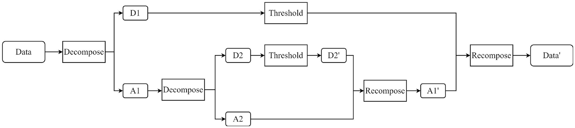
Wavelet decomposition and reconstruction with level 2.
The wavelet decomposition is shown in Equation 4.
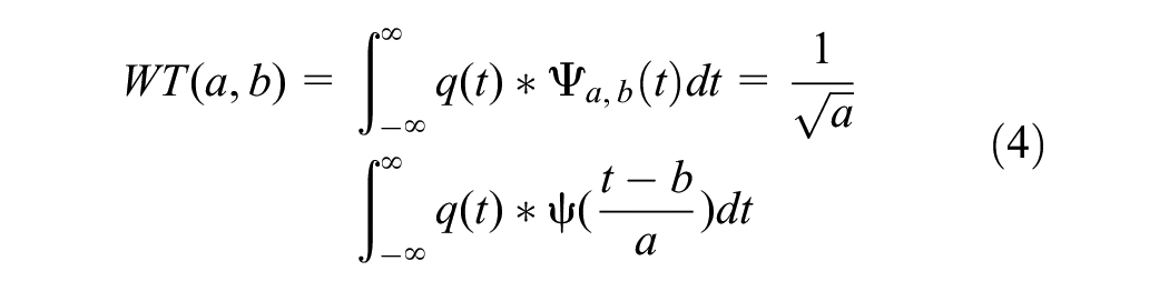
where
The wavelet analysis decomposes the high-frequency and low-frequency vectors of the original traffic flow data, and thresholds the high-frequency vector, and finally reconstructs into the noise reduction data. The detailed design is described below.
1) Wavelet basis function selection
For different types of data, different wavelet basis functions need to be selected. Wavelet basis function is defined as generated by translating and scaling the mother wavelet. The definition is shown in Equation 5.
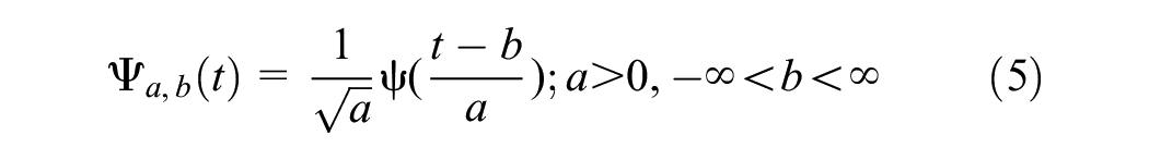
where
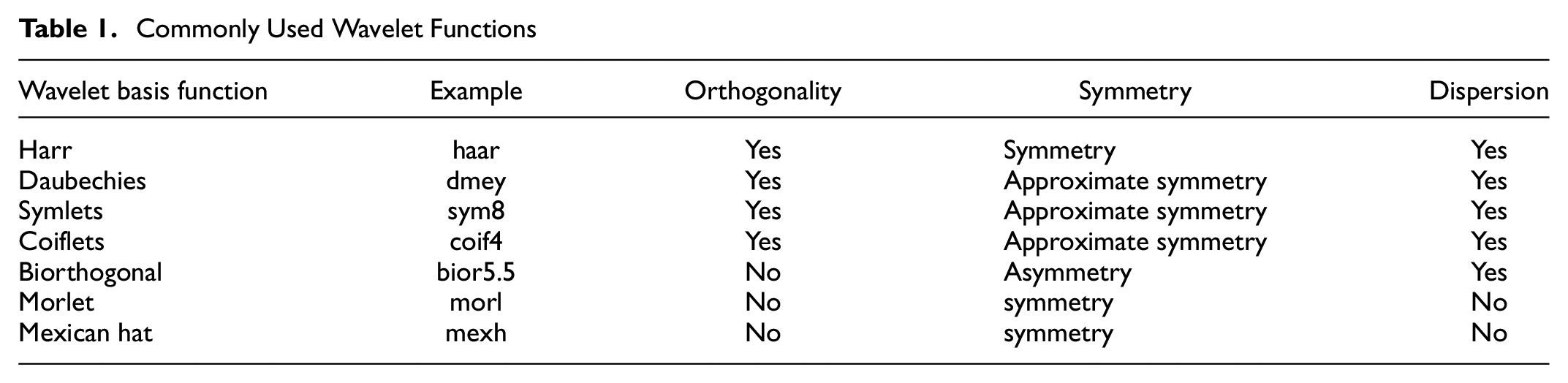
When dealing with the same problem, different types of wavelet basis functions may produce different results because of their unique time-frequency characteristics. Depending on the particular traffic flow in a specific problem, it is necessary to select the appropriate type, scale, and displacement of the wavelet basis functions. In this paper, the selection of wavelet basis functions is based on three main aspects: orthogonality, symmetry, and dispersion.
Orthogonal basis functions have better noise reduction performance in signal reconstruction. For noisy data, the independence of the coefficients helps to distinguish signal from noise more clearly. Orthogonal basis functions have better robustness to error and noise because there is no interdependence between them and the error is minimized in all directions. Symmetric wavelet basis functions avoid phase distortion in signal analysis and reconstruction because of their linear phase properties. The dispersion then refers to whether the wavelet basis functions support discrete wavelet transforms. The discrete wavelet transform is usually more efficient than the continuous wavelet transform because it eliminates redundant correlations between two points in wavelet space. Discrete wavelet transforms are also generally more robust and have better tolerance for noise and other forms of data perturbation. Table 1 compares the commonly used wavelet functions ( 42 ).
Commonly Used Wavelet Functions
In the experimental section we compare the prediction effects of various wavelet basis functions on traffic flow data after decomposition and reconstruction.
2) Decomposition level setting
Possible noise in the data needs to be analyzed and removed at different scales. Different levels of decomposition correspond to different scales of analysis. Each decomposition layer uses a different scale to measure the original signal, and the scale is gradually refined as the number of layers increases. To find the best decomposition level, the traffic flow prediction effect is judged according to the different decomposition levels after denoising.
3) Threshold processing method
In the process of WTD, the selection of the threshold value is a key step. The selection methods of wavelet thresholds generally include four criteria such as unbiased risk estimation thresholds, fixed thresholds, heuristic thresholds, and very large and very small thresholds.
Fixed thresholds are simple to compute, easy to implement and understand, but do not apply to noisy or complex data. Very large and very small thresholds, which are usually more robust since they are optimized in the worst case, do not perform optimally in general. Heuristic thresholds, which can be adapted to different types and complexities of data, do not have a clear theoretical basis to explain why this compromise works in specific scenarios. Using unbiased risk estimates such as Stein’s Unbiased Risk Estimate (SURE) for threshold selection have some characteristics and advantages. For example, they are unbiased; SURE provides an unbiased risk estimate, meaning you can more accurately gauge the predictive capabilities of your model. They are data driven; unlike some thresholding techniques, SURE is a data-driven method, requiring no a priori setting or manual selection of thresholds. They are adaptive; SURE can adaptively adjust the threshold based on the data, often leading to better predictive performance. They have real-time capabilities, for example, in some implementations, SURE can be calculated in real time, which is very useful for tasks like traffic prediction that often require quick responses. Finally, they are robust; because SURE is based on unbiased risk estimation, it usually offers better robustness to various types of noise and data distributions.
Therefore, this study adopted the unbiased risk estimation threshold (Rigrsure) principle: the new sequence

where
If the threshold is the square root of the

The risk generated by the threshold is
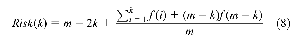
The value of

Threshold functions are selected to filter noisy wavelet coefficients and remove Gaussian noise; the most commonly used thresholding functions are soft and hard thresholding functions. By using soft thresholding, the curve of the data will be smoothed, and the noise will be removed as much as possible while retaining the valid information. Hard thresholding retains spike features and, although the denoising is more thorough, it can easily remove useful information that is mistaken for noise. Therefore, a soft threshold function is used in this study, which is defined as follows.
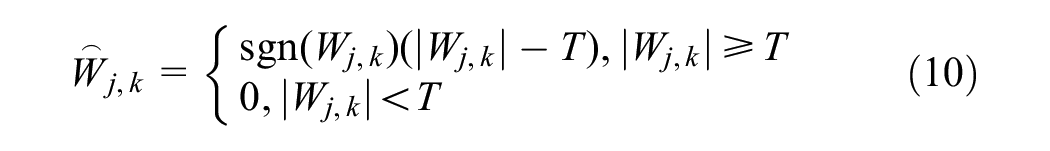
where
Prediction: Functional Principal Components Analysis
In this paper, we use the functional principal components analysis proposed by Wagner-Muns et al. ( 39 ) for traffic flow prediction. In contrast to Wagner-Muns et al. ( 39 ), we use Fourier basis functions to better fit the discrete time series. The FPCA steps are as follows.
Step 1. Fourier basis functions are used to fit the ICEEMDAN-WTD denoised and reconstructed traffic flow time series to generate function principal components and scores.
Step 2. The SARIMA model is used to fit each functional principal component’s score to produce a prediction of the next day’s principal components score.
Step 3. As time passes into the prediction day, the principal components’ scores for that day are estimated using some of the observations from the prediction day.
Step 4. The predicted principal components scores are combined with the estimated principal components scores to produce traffic flow predictions for the remainder of the day.
Step 5. Finally, the predicted values are compared with the observed values to determine the prediction interval.
Experiment
Data Source
The proposed model is validated using real traffic flow data from three intersections in Guiyang City, China. The three green dots in Figure 3 show the geographic locations of the three intersections. The data collection period is from March 1 to March 31, 2021. The detector collects data every 5 min, and 288 data are collected every day for 31 days. The data from the first 20 days of the three intersections are used as the training set, the data from 6 a.m. to midnight on the 21st day are used as the validation set, and the data from 6 a.m. to midnight on the 22nd day are used as the test set.
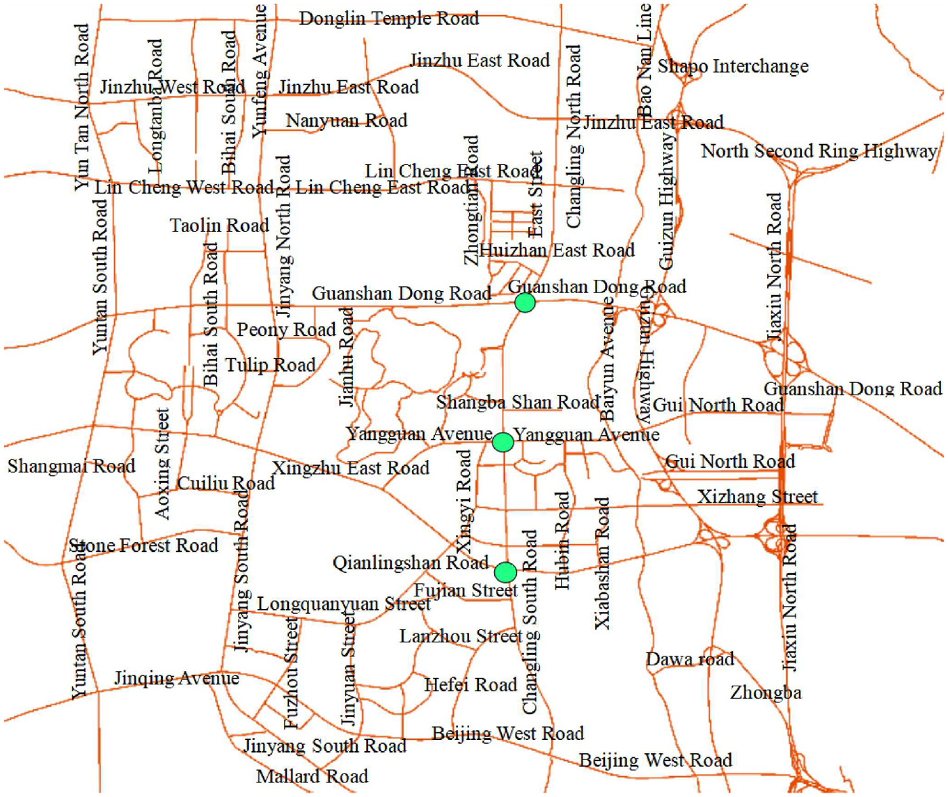
Distribution of observation points.
We used the “statsmodels” and “SciPy” modules of Python to test the smoothness, autocorrelation, normality, randomness, and nonlinearity of the data set. First, Augmented Dickey–Fuller (ADF) test was used to test the smoothness of the data. The zero order ADF results show a
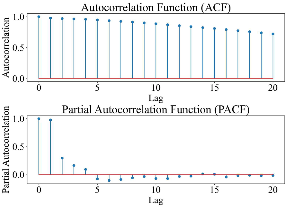
Autocorrelation function (ACF) and partial autocorrelation function (PACF) of traffic flow data.
Data tests show that the traffic flow time-series data are smooth, autocorrelated, do not obey normal distribution and are non-random and nonlinear. These data contain a lot of noise. As a result, traditional prediction models will have difficulty predicting traffic flow with high accuracy without using correlation methods for noise reduction on the raw data ( 4 – 6 ). The results of the relevant experimental data are shown in Table 2.
Statistical Description of Data
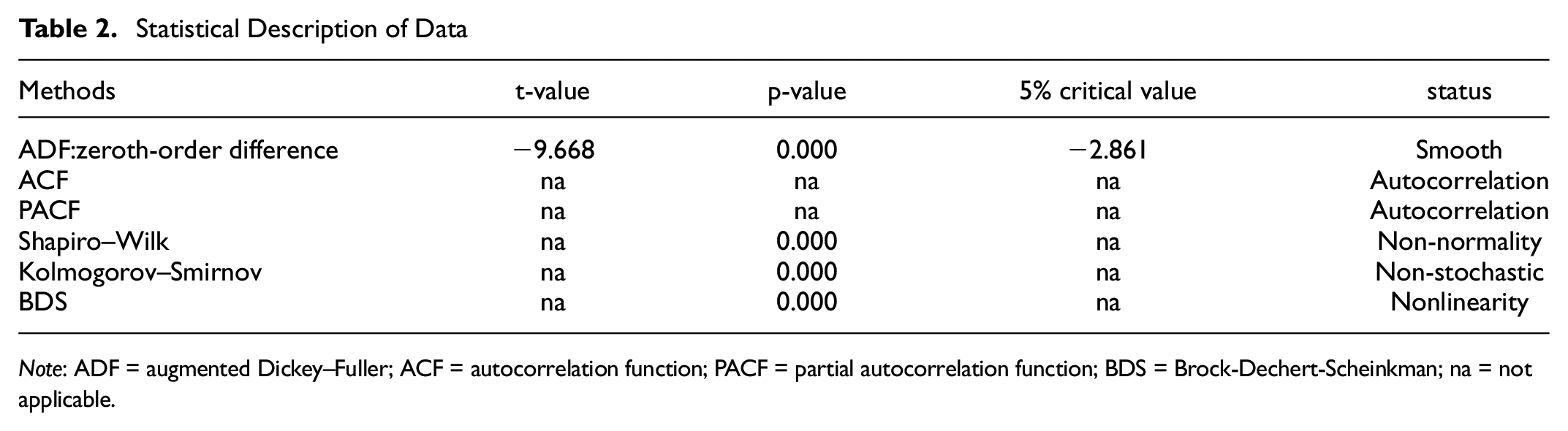
Note: ADF = augmented Dickey–Fuller; ACF = autocorrelation function; PACF = partial autocorrelation function; BDS = Brock-Dechert-Scheinkman; na = not applicable.
Experimental Environment and Performance Indicators
The experimental environment was a server (CPU: Intel(R) Core(TM) i5-10500, GPU: Inter(R) UHD Graphics 630 16 GB).
To evaluate the prediction performance of the model, we used two metrics: root mean square error (RMSE) and mean absolute error (MAE).
Here are the reasons why we chose RMSE and MAE.
1) Interpretable units: Both RMSE and MAE are in the original units of the data, making them more interpretable.
2) No issues at zero: RMSE and MAE are always defined, unlike MAPE which can be infinite.
The definitions are as follows.
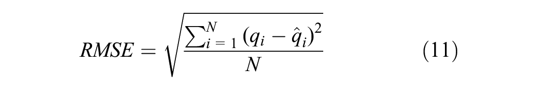

where
Since pure traffic flow data are not available to calculate the SNR, we use statistical metrics such as standard deviation (SD), variance (Var), and coefficient of variation (CV) to quantify and evaluate the noise level in the data. We use the percentage of noise reduction (PR) to measure the noise reduction effect.
The definitions are as follows.
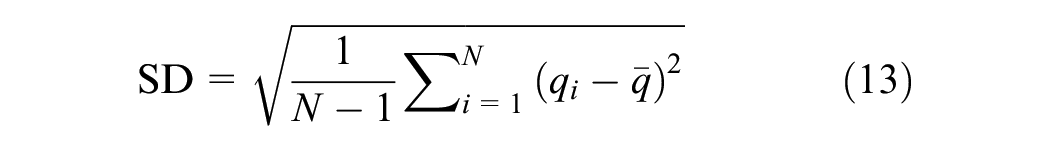


where
ICEENDAN-WTD Denoising Method
The original traffic flow data are decomposed using the ICEEMDAN algorithm. The noise standard deviation, number of realizations, and the maximum number of iterations need to be set in the ICEEMDAN decomposition. We chose the recommended value of 0.2 for the noise standard deviation ( 43 , 44 ). Colominas et al. ( 40 ) obtained the best decomposition results in ICEEMDAN using several realizations of 50. We, therefore, chose the number of realizations as 50. The maximum number of iterations is the value that ensures that a sufficient number of iterations are available for convergence. To fulfill this criterion, a large value of this parameter is required. Therefore, in this paper the maximum number of iterations is chosen as 500. The final ICEEMDAN decomposition gives 13 IMFs. Next, we will screen the IMFs using the correlation coefficient and autocorrelation function.
The correlation coefficients between each IMFs and the original signal are calculated separately, and the results are shown in Figure 5. From Figure 5, the correlation coefficient of the third IMFs takes a very small value for the first time, so IMF3 is the cut-off point and the high-frequency noise, and IMF1-IMF3 is considered as the noise IMFs.
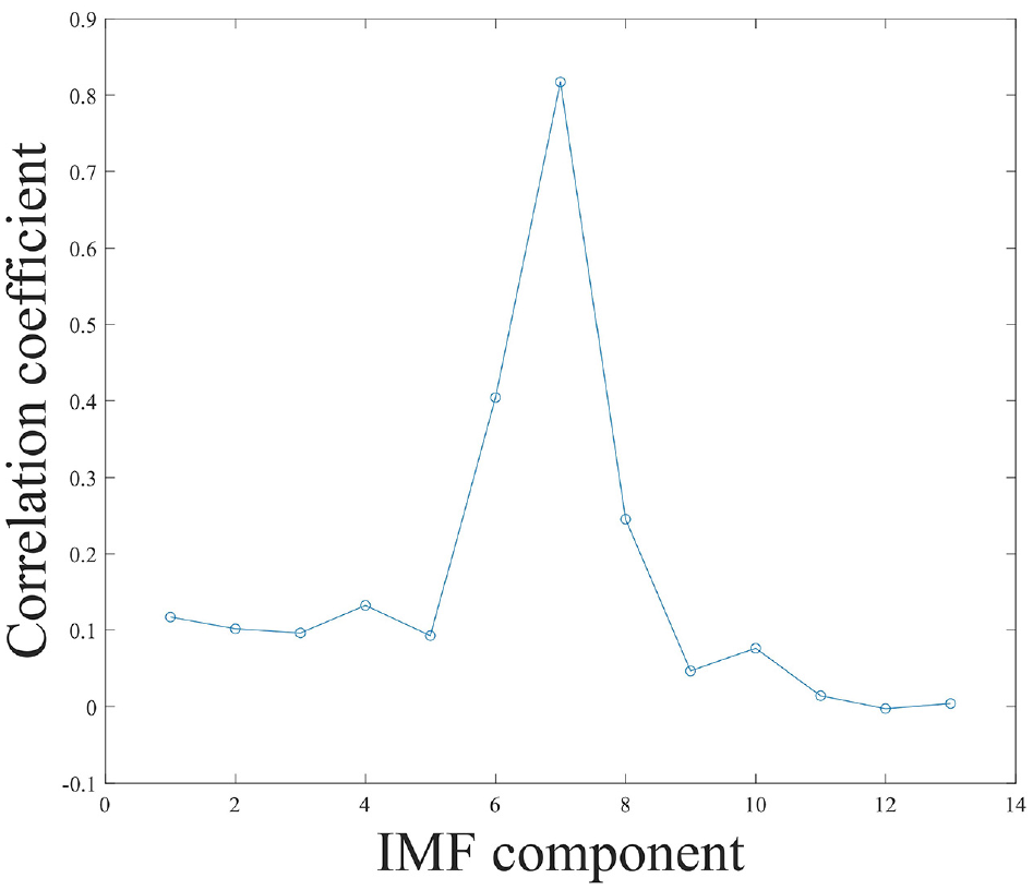
Correlation coefficient of each IMFs.
At the same time, the autocorrelation function of the noisy IMFs is used to achieve the screening of the IMFs by taking advantage of the rapid decay of the autocorrelation function near the zero point. The results of the normalized autocorrelation function for the first four IMFs are shown in Figure 6. According to Figure 6, IMF1-IMF3 take the maximum value at the zero point and then decay rapidly on both sides of the zero point, which indicates that these three IMFs contain noise. Based on the screening results of correlation coefficient and normalized autocorrelation function, the first three IMFs are selected for WTD treatment.

Normalized autocorrelation functions of the first four IMF: (a) IMF1, (b) IMF2, (c) IMF3, and (d) IMF4.
To better use WTD to reduce the effect of noise on traffic flow data, we need to determine the parameters of WTD in advance, including threshold, decomposition level, and wavelet basis function. We, therefore, conducted a series of experiments to compare the effects of two different thresholding methods (soft thresholding and hard thresholding), different decomposition levels, and different wavelet basis functions on denoising traffic flow data. These experiments aim to find out the most suitable WTD parameter configuration for processing traffic flow data. WTD(db4) is denoted as wavelet threshold denoising based on db4.
The possible noise in the data needs to be analyzed and removed at different decomposition scales, and we tested different decomposition levels of WTD to find the best decomposition level. Results are presented in Table 3. In Table 3,
Performance of Various Level of Wavelet Decomposition Models in WTD(coif3)
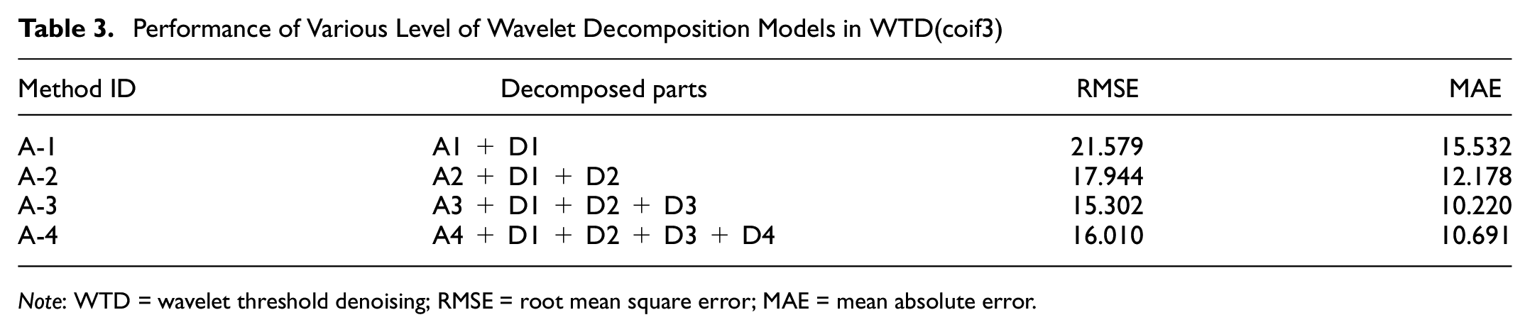
Note: WTD = wavelet threshold denoising; RMSE = root mean square error; MAE = mean absolute error.
The appropriate thresholding method is also one of the important influencing factors in the wavelet thresholding denoising process, so we compared the two methods of soft and hard thresholding for WTD, and the results are shown in Table 4. The results show that soft thresholding is more suitable for processing traffic flow data than hard thresholding. Soft thresholding makes the time series smoother and removes as much noise as possible while retaining valid information.
Comparison of Wavelet Basis Function
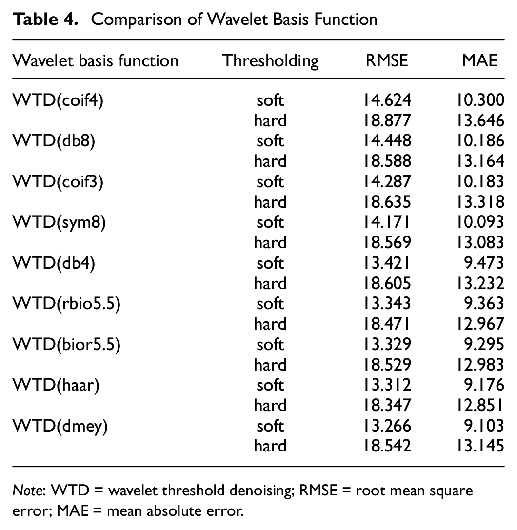
Note: WTD = wavelet threshold denoising; RMSE = root mean square error; MAE = mean absolute error.
Since wavelet basis functions play a key role in data denoising, as emphasized in a previous study ( 45 ), it is worth considering the unique properties of different wavelet bases when dealing with complex and highly noisy traffic data. coif3 and coif4 have good time and frequency localization properties and are particularly suitable for processing complex and noisy non-stationary signals. db4 and db8 are suitable for capturing abrupt changes and high-frequency components in traffic flow data, which helps to accurately predict traffic congestion or accidents. sym8 given its symmetry, it may be more appropriate for applications where the signal needs to be reconstructed or where phase distortion is to be avoided. dmey is typically used for more complex signal analysis and is suitable for the identification of periodicities and trends in traffic flow data. Haar wavelets are often used for fast analysis and real-time prediction because of their simplicity, but may not be applicable to complex traffic flow patterns. bior5.5 and rbio5.5 provide a flexible way to balance time and frequency resolution that may be applicable to a variety of complex traffic flow scenarios.
So, if we are concerned with high-frequency events such as traffic congestion, we might choose db4 or sym8; if we are more concerned with trends and periodicity, we might be inclined to use the dmey or coif series. Overall, a suitable choice of wavelet basis functions can significantly improve the accuracy and robustness of the traffic flow prediction model. Therefore, we compared the prediction performance of WTD based on nine different wavelet basis functions (coif 3, coif 4, db 4, db8, haar, bior5.5, rbio5.5, dmey, sym 8), to select a suitable wavelet basis function for denoising traffic flow data.
Table 4 gives the prediction results of the original traffic flow data based on different wavelet basis functions. dmey ( 46 ) indeed obtained the best prediction performance. The prediction accuracy of coif and sym types is higher and similar, because these two types of wavelet basis functions are more effective in dealing with data with symmetric features. Therefore, coif and sym also have better results. Tang et al. ( 47 ) proposed that the db-type also shows a good fitting effect on the variation pattern of traffic flow data.
From the above analysis, we conclude that the decomposition level of WTD is chosen to be 3, the threshold value is chosen to be soft threshold, and the wavelet basis function is chosen to be dmey. Next, we use the optimal parameters of WTD for noise reduction of the first three IMFs.
The wavelet basis function is selected as dmey, the decomposition level is set to 3, the threshold method of IMF1 is set to fixed threshold, and the threshold function is selected as hard threshold function. The threshold method for IMF2-IMF3 is set to the unbiased risk estimation threshold (Rigrsure) principle, and the threshold function is chosen as a soft threshold function, while retaining the other IMFs.
The results of WTD are shown in Figure 7. It can be seen from Figure 7 that the noise contained in IMF1-IMF3 is effectively removed after the WTD treatment.
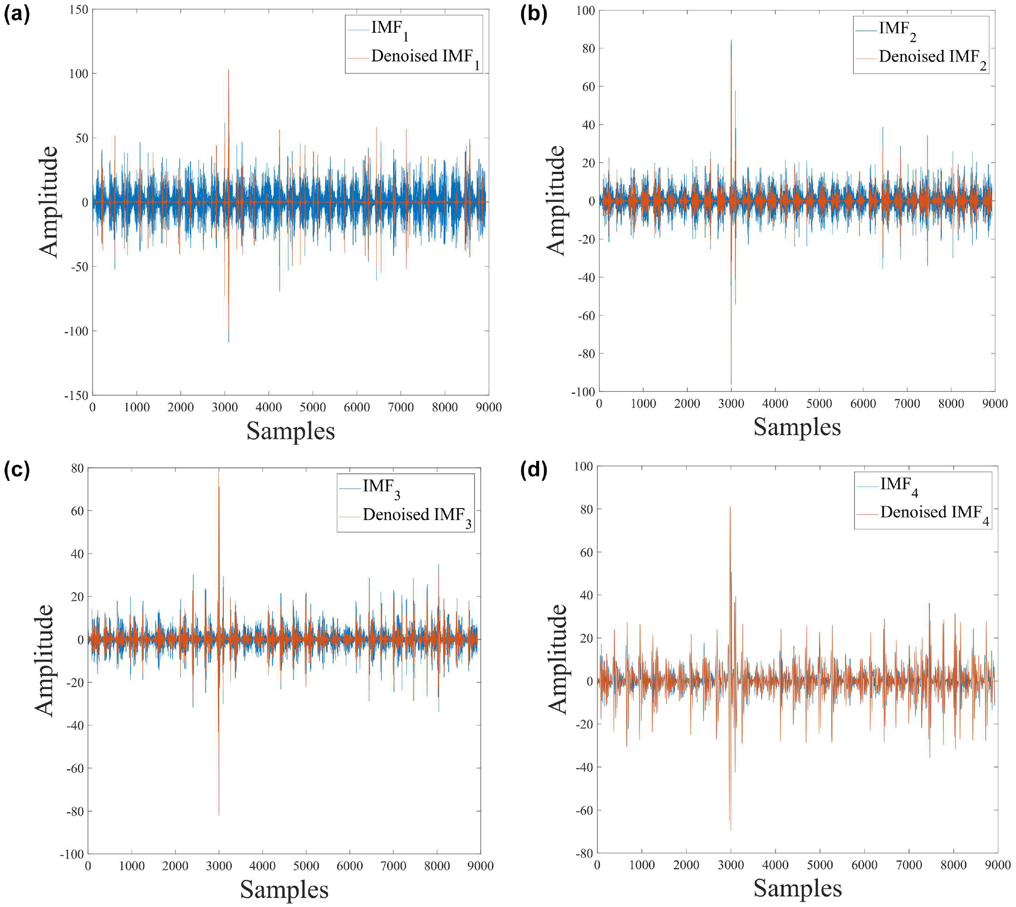
Wavelet threshold denoising effect: (a) IMF1, (b) IMF2, (c) IMF3, and (d) IMF4.
To verify the effectiveness of the screening method, the IMF4 was processed with WTD, and it was found that there is almost no change between the IMF4 and the original IMF4 after noise reduction. This shows that there is almost no noise in the IMF4, indicating the effectiveness of the screening method.
To illustrate the effectiveness of ICEEMDAN-WTD method, the prediction performance, reconstruction error, and decomposition time are compared with WTD(dmey), EMD, EEMD, CEEMDAN, and ICEEMDAN using ICEEMDAN-WTD respectively.
The prediction results are shown in Table 5. The experimental results show that ICEEMDAN-WTD obtains the highest prediction accuracy. The denoising methods are ranked in order of prediction error from best to worst: ICEEMDAN-WTD > ICEEMDAN > CEEMDAN > EEMD > WTD(dmey) > EMD. Although ICEEMDAN shows some advantages by avoiding spurious patterns and reducing the noise contained in the patterns, ICEEMDAN only outperforms the other methods in most cases. For other cases, see Supplemental material (Tables S1–S3).
Comparison of Denoising Effect of Denoising Methods
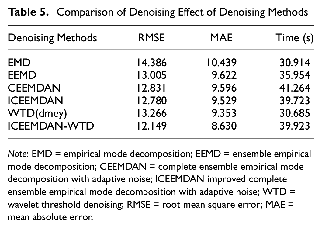
Note: EMD = empirical mode decomposition; EEMD = ensemble empirical mode decomposition; CEEMDAN = complete ensemble empirical mode decomposition with adaptive noise; ICEEMDAN improved complete ensemble empirical mode decomposition with adaptive noise; WTD = wavelet threshold denoising; RMSE = root mean square error; MAE = mean absolute error.
In addition, the time required for prediction varies because of the different strategies employed by different decomposition methods in processing the noise and performing the decomposition. ICEEMDAN-WTD has a slightly longer prediction time compared with several other methods, but the prediction accuracy of the model is somewhat improved.
The reconstruction errors of the decomposition methods are shown in Table 6. The reconstruction error is the largest given the presence of mode mixing in EMD. EEMD reduces mode mixing by adding white noise, so lower reconstruction errors than EMD are obtained. CEEMDAN further optimizes the noise handling mechanism to obtain relatively low reconstruction errors. ICEEMDAN, as an improvement of CEEMDAN, improves the quality of the decomposition by further optimizing the decomposition process and obtains the lowest reconstruction error. Therefore, the negligible reconstruction error leads to improved prediction performance of ICEEMDAN-based models compared with EMD, EEMD, and CEEMDAN.
Reconstruction Error of Decomposition Methods
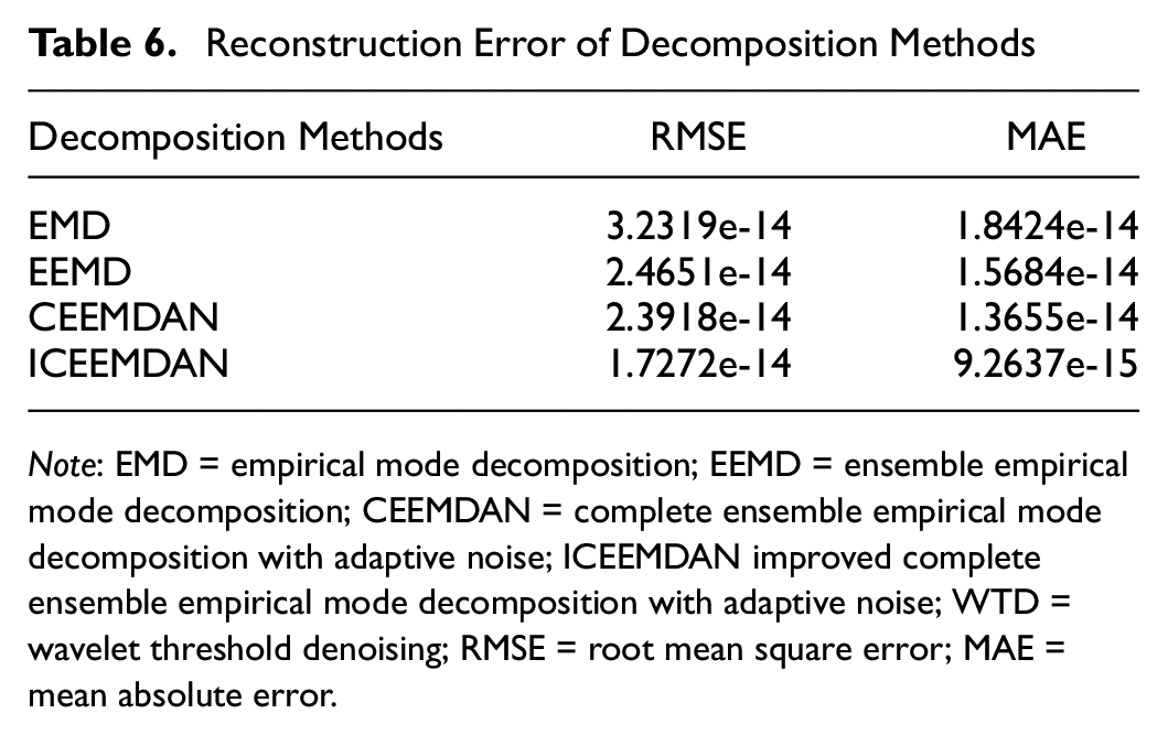
Note: EMD = empirical mode decomposition; EEMD = ensemble empirical mode decomposition; CEEMDAN = complete ensemble empirical mode decomposition with adaptive noise; ICEEMDAN improved complete ensemble empirical mode decomposition with adaptive noise; WTD = wavelet threshold denoising; RMSE = root mean square error; MAE = mean absolute error.
The decomposition times of the denoising methods are shown in Table 7. For decomposition time we used the average of 10 decomposition times as the result. The decomposition time of EMD is only 0.4 s. EMD has the shortest decomposition time given that it directly decomposes the given data without additional iterations or integration processes. The EEMD decomposition time is 5.4 s. EEMD requires more time for decomposition because it improves the results by adding different white noise and performing multiple decompositions and averaging. The decomposition time of CEEMDAN is 10.7 s. The decomposition time of CEEMDAN is usually longer than that of EMD and EEMD. This is a result of CEEMDAN needing to adaptively adjust to the noise during the decomposition process, an extra step that increases the computational burden. The decomposition time of ICEEMDAN is 9.2 s. ICEEMDAN also usually requires a longer decomposition time as a result of the iterative approach used to minimize the reconstruction error. Each iteration requires the completion of a full decomposition and reconstruction process, which significantly increases the computation time. WTD is usually faster compared with EMD and its variants. Wavelet methods are well localized in both the frequency and time domains, which makes it fast to identify and remove noise. Fortunately, the proposed ICEEMDAN-WTD method is acceptable although it has a slightly longer running time.
Decomposition Time of Denoising Methods
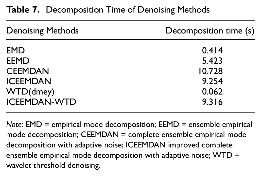
Note: EMD = empirical mode decomposition; EEMD = ensemble empirical mode decomposition; CEEMDAN = complete ensemble empirical mode decomposition with adaptive noise; ICEEMDAN improved complete ensemble empirical mode decomposition with adaptive noise; WTD = wavelet threshold denoising.
Functional Principal Components Analysis
In this section, we combine FPCA with the ICEEMDAN-WTD denoising method, denoted as ICEEMDAN-WTD-FPCA. And the performance of the proposed model is verified through comparative experiments.
Fit the Basis Function to the Denoised Traffic Flow Data
The Fourier basis function is first used to fit the discrete traffic flow time series reconstructed by ICEEMDAN-WTD denoising. The smoothing penalty parameter
Generation of Functional Principal Components
Although a smooth function representation of the discrete time series has been constructed, this treatment results in strong correlation between the Fourier basis functions. Correlations between them are analyzed by functional principal components to decrease the dimensionality of the data and to denote their predictable patterns of variation. The first four principal components are determined to represent 95% of the variation in the functional time-series data by the variance contribution. When generating predictions, the use of FPCA to reduce the variability of the data makes the model more robust to transient changes in traffic. FPCA retains the main patterns of change in the data. In many cases, the first principal component function corresponds directly to a clearly observable phenomenon in the data ( 48 ).
In Figure 8, it can be seen that their peak periods are consistent. Each day in the original data set needs to be described by 288 values, while each FPCA needs only four values to represent the traffic flow of a day. This reduces the dimensionality and relevance of the data set and reduces the complexity of prediction.
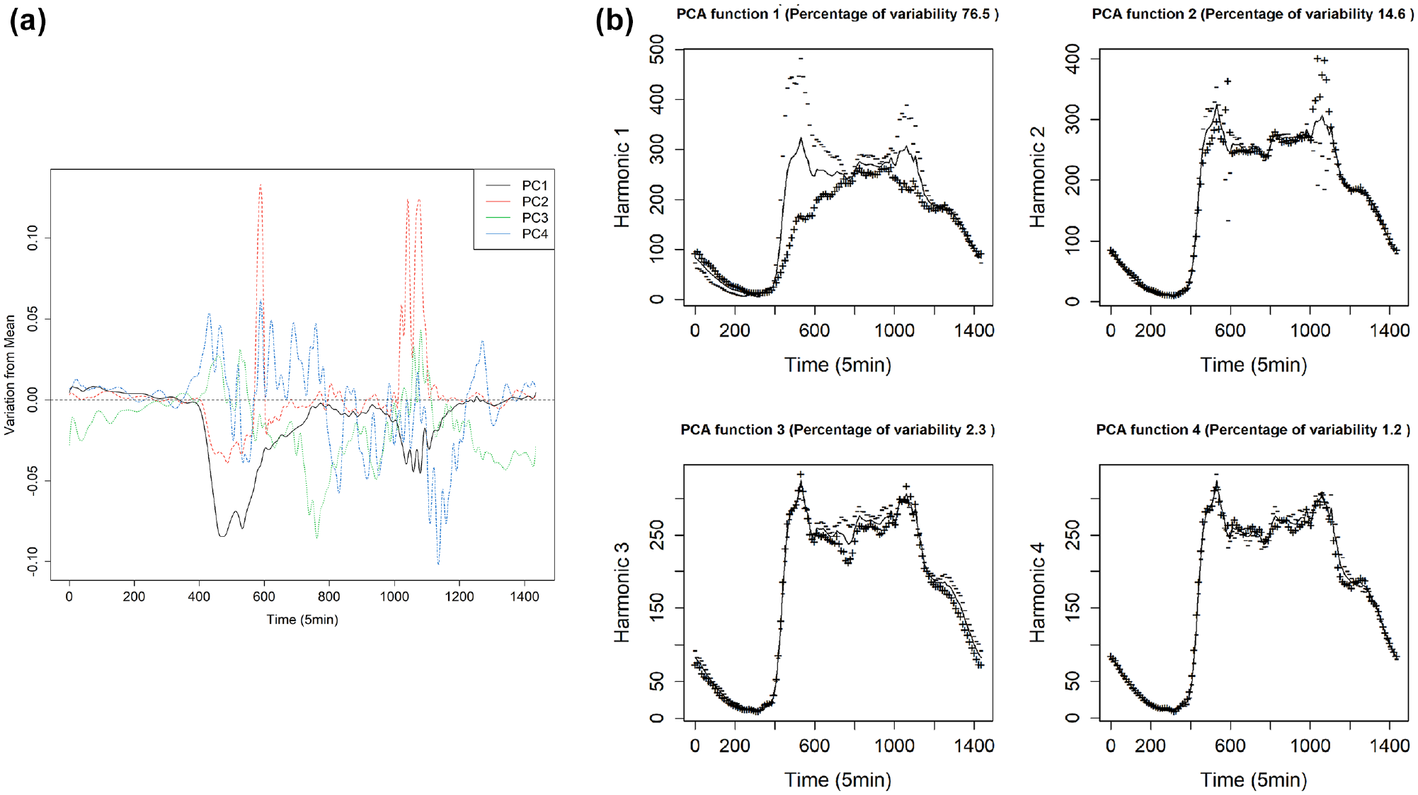
FPCA harmonics modify the mean function: (a) FPCA harmonics and (b) 4 FPCA harmonic modifying mean function.
Fitting Principal Component Scores Using SARIMA Model
The FPCA scores for the past 21 days are used to determine the parameters of the SARIMA model. The model parameters are determined automatically using the auto.arima function in R. We select the model parameters that minimize the AIC. Finally, the models corresponding to the first four FPCA scores are SARIMA(2, 0, 0)(0, 1, 0)5, SARIMA(2, 0, 0)(0, 1, 0)5, SARIMA(1, 0, 0)(0, 1, 0)5, SARIMA(3, 1, 0)(0, 1, 0)5. These SARIMA models will generate the FPCA score predictions for the next day.
Generate Prediction and Performance Comparison
Although the SARIMA model is able to produce accurate predictions of traffic behavior for the next day, it does not take into account new data as time passes into the forecast day ( 39 ). New information from some of the prediction days will be used to estimate the FPCA score for that day. We use the traffic flow data for the first 6 h of the forecast day to estimate the principal component scores for that day. The output principal component score prediction is the weighted average of the scores generated by the SARIMA model prediction and the cumulative standard deviation of the estimated scores from the partially observed traffic flow information. Lastly, the weighted average score is transformed into a functional representation to produce traffic flow forecasts for the rest of the day.
Next, the denoising effect of the denoising method ICEEMDAN-WTD and the prediction performance of the proposed framework ICEEMDAN-WTD-FPCA are verified through comparative experiments on different types of data sets. Tables 9–11 show the predictive performance of the different models, with the best performance highlighted in bold. We compare SARIMA, SVR, LSTM, GRU, and FPCA models and also compare the prediction performance of SARIMA and FPCA based on different denoising methods: WTD(dmey), EMD, EEMD, CEEMDAN, ICEEMDAN, and ICEEMDAN-WTD. The model parameters of SVR, LSTM, and GRU are determined by using stochastic search ( 49 ). Specifically, the names of the hyperparameters and their corresponding optimal values are shown in Table 8.
The Names of the Tuned Hyperparameters in the Model and Their Corresponding Optimal Values
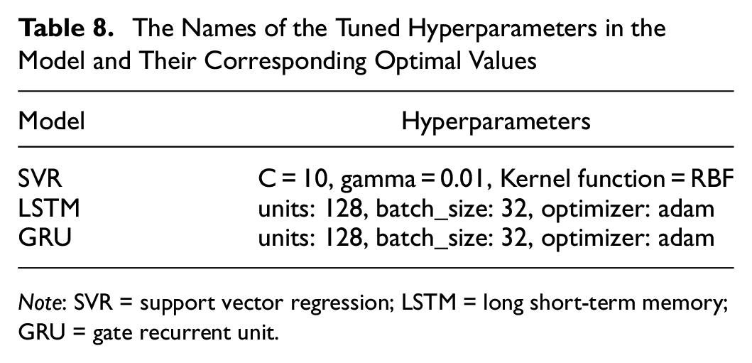
Note: SVR = support vector regression; LSTM = long short-term memory; GRU = gate recurrent unit.
Performance Comparison of Different Methods for Changling South Road and Yangguan Avenue
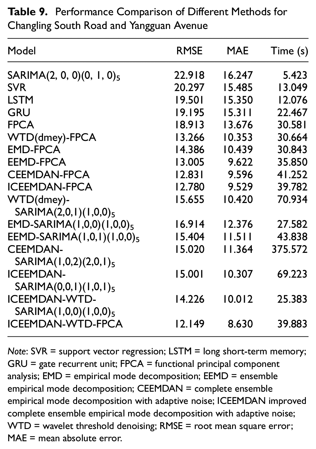
Note: SVR = support vector regression; LSTM = long short-term memory; GRU = gate recurrent unit; FPCA = functional principal component analysis; EMD = empirical mode decomposition; EEMD = ensemble empirical mode decomposition; CEEMDAN = complete ensemble empirical mode decomposition with adaptive noise; ICEEMDAN improved complete ensemble empirical mode decomposition with adaptive noise; WTD = wavelet threshold denoising; RMSE = root mean square error; MAE = mean absolute error.
Performance Comparison of Different Methods for Changling South Road and Qianlingshanlu Road
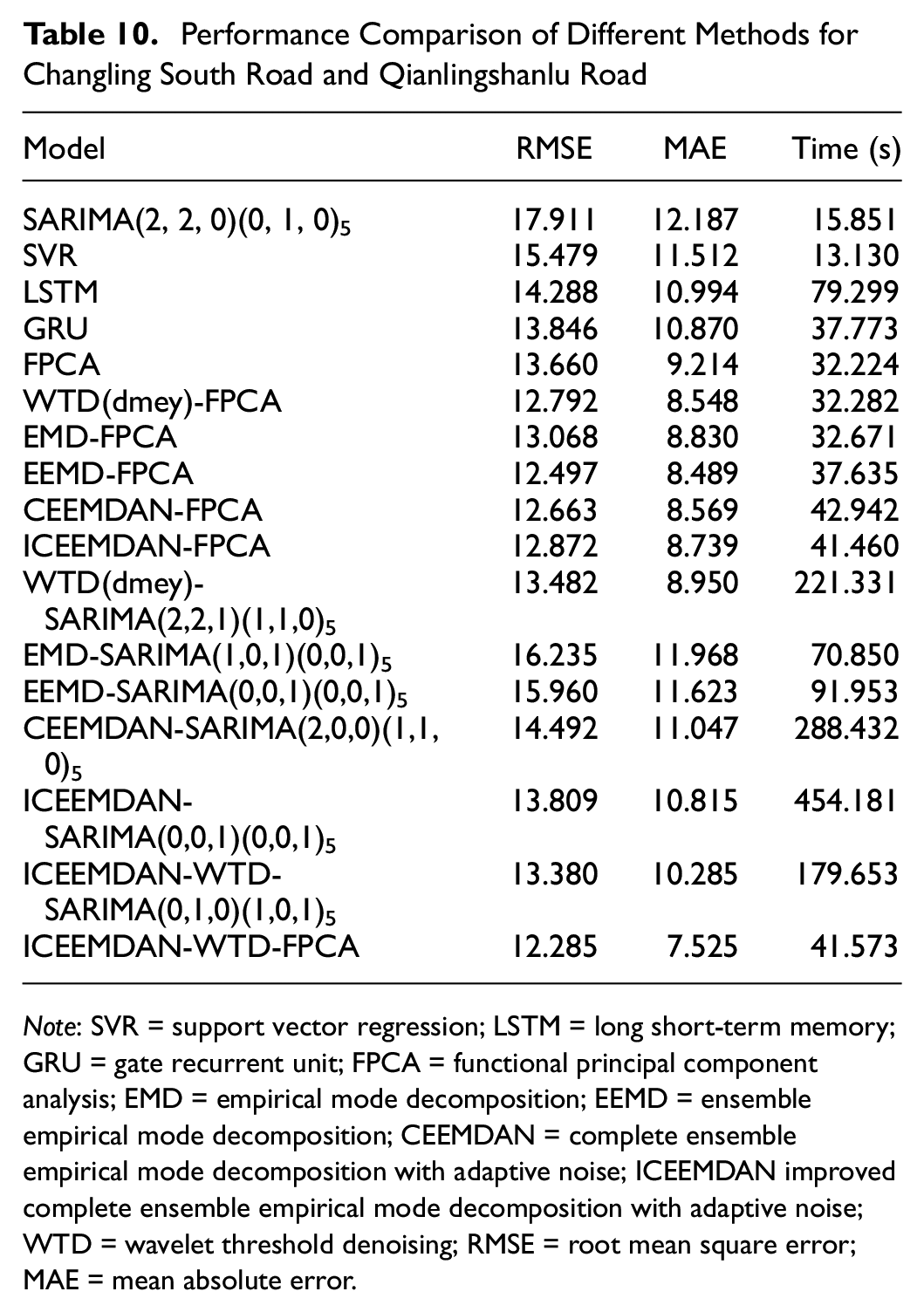
Note: SVR = support vector regression; LSTM = long short-term memory; GRU = gate recurrent unit; FPCA = functional principal component analysis; EMD = empirical mode decomposition; EEMD = ensemble empirical mode decomposition; CEEMDAN = complete ensemble empirical mode decomposition with adaptive noise; ICEEMDAN improved complete ensemble empirical mode decomposition with adaptive noise; WTD = wavelet threshold denoising; RMSE = root mean square error; MAE = mean absolute error.
Performance Comparison of Different Methods for Changling North Road and Guanshandonglu Road
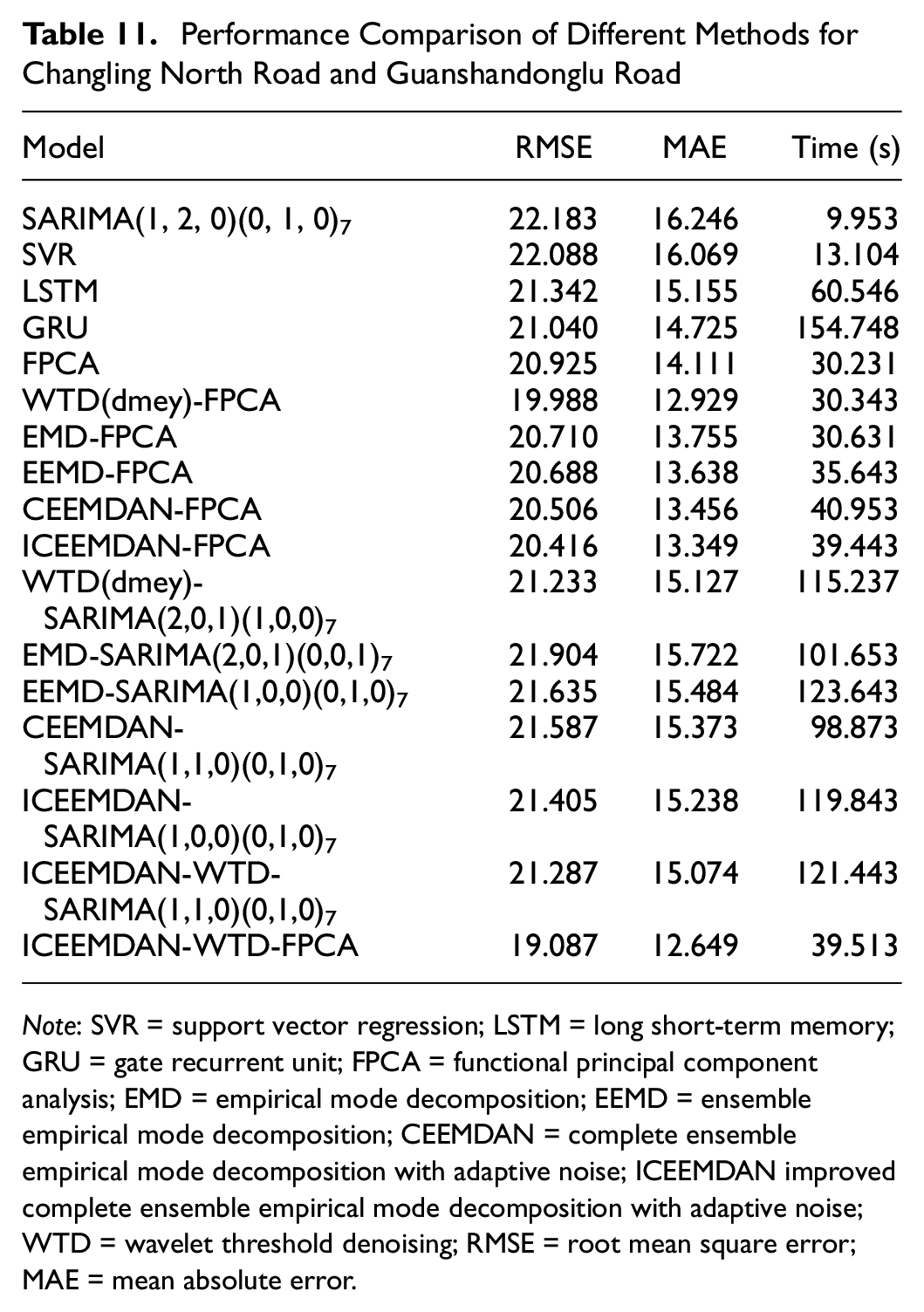
Note: SVR = support vector regression; LSTM = long short-term memory; GRU = gate recurrent unit; FPCA = functional principal component analysis; EMD = empirical mode decomposition; EEMD = ensemble empirical mode decomposition; CEEMDAN = complete ensemble empirical mode decomposition with adaptive noise; ICEEMDAN improved complete ensemble empirical mode decomposition with adaptive noise; WTD = wavelet threshold denoising; RMSE = root mean square error; MAE = mean absolute error.
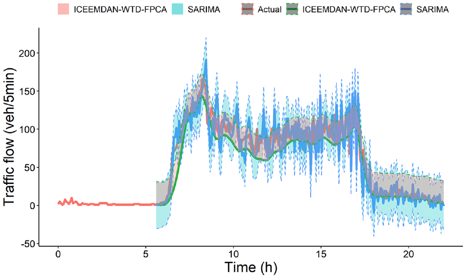
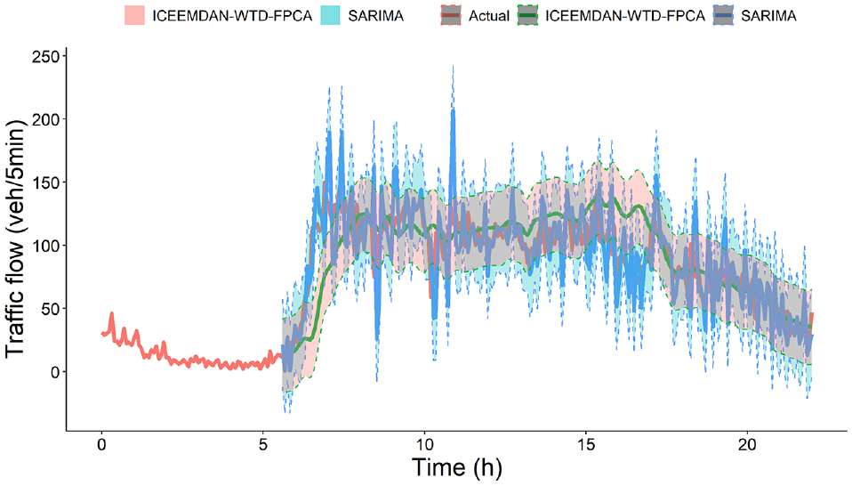
Based on the prediction results given in Tables 9–11 and Figures 9–11, some interesting findings can be summarized.
1) The SARIMA model performs worse than other models, indicating that the traditional linear model cannot capture the evolutionary characteristics of short-time traffic flow.
2) Compared with the discrete SARIMA model, the FPCA model has a higher prediction accuracy and is more robust to transient events in the traffic flow.
3) The forecast interval of the functional forecast is more consistently narrower because it forecasts the future in fewer steps, and it incorporates weekly seasonality into the forecast without discrimination.
4) Traditional time-series models for traffic flow forecasts for the remaining days consist of point forecasts generated by multiple iterations. In contrast, the time-series model based on FPCA forecasts for a whole day is a single point forecast for the future.
5) The FPCA model outperforms the classical machine learning model SVR and the deep learning models LSTM and GRU, indicating that FPCA is an effective traffic flow prediction model.
6) The results in Table 10 show that the prediction performance based on ICEEMDAN does not perform as well as that based on EEMD, which is consistent with the results we obtained from analyzing them for noise reduction effect.
7) Although the ICEEMDAN-WTD-based model takes a little longer to generate predictions, the prediction accuracy is significantly improved, which is acceptable.
8) Among the prediction models based on WTD(dmey), EMD, EEMD, CEEMDAN, ICEEMDAN, and ICEEMDAN-WTD, the model based on ICEEMDAN-WTD has the highest prediction accuracy. It shows that it can effectively reduce the noise disturbance and improve the model prediction performance.
9) The prediction results of the models combined with the denoising method are better than those without the denoising method, indicating that the decomposition algorithm and the data denoising process can reduce the influence of noise on the prediction models.
10) The ICEEMDAN-WTD-FPCA model proposed in this paper has the lowest RMSE and MAE, indicating that the ICEEMDAN-WTD-FPCA model is an effective model for traffic flow prediction.
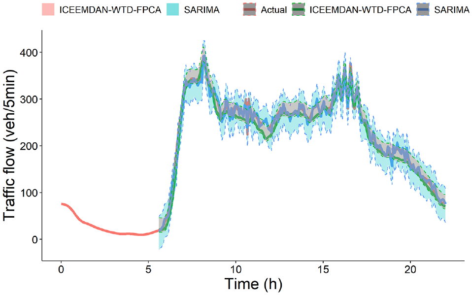
ICEEMDAN-WTD-FPCA and SARIMA with 90% prediction intervals starting 6 h into the day for Changling South Road and Yangguan Avenue.
ICEEMDAN-WTD-FPCA and SARIMA with 90% prediction intervals starting 6 h into the day for Changling South Road and Qianlingshanlu Road.
ICEEMDAN-WTD-FPCA and SARIMA with 90% prediction intervals starting 6 h into the day for Changling North Road and Guanshandonglu Road.
Conclusions
In this paper, an ICEEMDAN-WTD-FPCA framework combining data denoising and prediction is proposed to achieve traffic flow prediction. For traffic flow data disturbed by different noise, we propose a new data denoising method ICEEMDAN-WTD to remove noise and reconstruct to improve data quality. This method is also combined with FPCA to predict the trend of traffic flow. The conclusions are summarized as follows.
1) The ICEEMDAN-WTD-FPCA model proposed in this paper significantly improves the performance of traffic flow prediction. It shows that the proposed model is an effective method for traffic flow prediction.
2) Unlike other prediction methods, we use the potential function characteristics of the traffic flow time series for traffic flow prediction.
3) We have combined the advantages of different decomposition and denoising methods to propose an ICEEMDAN-WTD denoising method. The ICEEMDAN-WTD method significantly improves the predictive performance of the model over other methods.
4) We have compared the denoising effects of various smoothing models (EMD, EEMD, CEEMDAN, ICEEMDAN and WTD) on traffic flow data. We provide a reference for selecting denoising methods for traffic flow data.
In future work, we will try to improve the model in three ways.
1) This paper uses the SARIMA model to predict daily FPCA scores, however, methods such as neural networks and support vector machines can also be used in place of SARIMA to predict daily FPCA scores. Perhaps these models will outperform SARIMA in producing predictions.
2) The prediction model FPCA used in this paper provides some new ideas for traffic flow prediction with higher prediction accuracy compared with commonly used statistical methods. However, the prediction can be further improved by incorporating complex nonlinear factors, such as combining the proposed method with deep learning models.
3) We will focus on how well the proposed method handles unusual/unforeseen events such as weather, accidents, and other disruptions. This might be an interesting topic for future research.
Supplemental Material
sj-pdf-1-trr-10.1177_03611981241242375 – Supplemental material for Traffic Flow Prediction by an Ensemble Framework with Data Denoising and Functional Principal Components Analysis
Supplemental material, sj-pdf-1-trr-10.1177_03611981241242375 for Traffic Flow Prediction by an Ensemble Framework with Data Denoising and Functional Principal Components Analysis by Yutao Qin, Chuliang Wu and Yao Hu in Transportation Research Record
Footnotes
Author Contributions
The authors confirm contribution to the paper as follows: study conception and design: Yutao Qin; data collection: Yutao Qin; analysis and interpretation of results: Yutao Qin; draft manuscript preparation: Yutao Qin, Chuliang Wu, Yao Hu. All authors reviewed the results and approved the final version of the manuscript.
Declaration of Conflicting Interests
The author(s) declared no potential conflicts of interest with respect to the research, authorship, and/or publication of this article.
Funding
The author(s) disclosed receipt of the following financial support for the research, authorship, and/or publication of this article: This work was supported by the National Natural Science Foundation of China (Grant No. 12161016 and No. 11661018) and the Guizhou Provincial Basic Research Program (Natural Science) (No. QianKeHeJiChu-ZK[2024]YiBan082).
Supplemental Material
Supplemental material for this article is available online.
References
Supplementary Material
Please find the following supplemental material available below.
For Open Access articles published under a Creative Commons License, all supplemental material carries the same license as the article it is associated with.
For non-Open Access articles published, all supplemental material carries a non-exclusive license, and permission requests for re-use of supplemental material or any part of supplemental material shall be sent directly to the copyright owner as specified in the copyright notice associated with the article.