Using Machine Learning to Predict Axial Pile Capacity

Abstract

Accurate estimation of the ultimate axial load bearing capacity of piles is necessary to ensure the safety of the supported structures and to prevent cost overruns. Traditional mechanics-based design methods do not always predict pile capacity accurately, or precisely, leaving room for improvement. This study focuses on the potential of machine learning (ML) in estimating pile capacity. A dataset of 546 load tests was compiled from three databases. The baseline performance of traditional design methods was first established by comparing the capacities computed using four traditional approaches, against the capacities interpreted from load tests using Davisson’s criterion. Sixteen different ML techniques were explored. First, the optimal feature selection technique for model training was investigated. Second, hyperparameters of each technique were optimized. The process involved the training of 32,000 different models and tuning their hyperparameters. Next the dataset was randomly split into training (70%) and testing (30%) for comparing the 16 different ML regression models. Each of the optimized models was then trained using six feature sets. The performance of each of the 16 ML models with the best performing feature subset was compared with the baseline performance from traditional methods. Evaluation criteria included measured versus predicted capacities, influence of soil type on accuracy, as well as the absence of pile diameter, or length effects on accuracy and precision. In general, the ML methods performed significantly better than the best traditional method. The current research demonstrated that ML may offer advantages in geotechnical design when large datasets are available.

Keywords

artificial intelligence data and data science foundations infrastructure machine learning (artificial intelligence)piles

Empirical and semi-empirical methods are commonly used for the design of driven piles. Capacity is typically calculated following a series of recommended design steps that are intended to generalize the experience gained from conducting load tests on piles. These approaches typically employ load test data to calibrate a mechanics-based design framework. Recent studies investigating the efficacy of some of the most commonly used design methods revealed that the performance of those methods is concerning (1 –3). The main problem stems from the small size of the databases used for the original development of these design approaches. In addition, load tests are costly and time-consuming, so nearly all methods rely on tests, of varying quality, typically reported by others. Finally, few of these design methods adequately account for changes in soil properties and the redistribution of stresses from pile driving. It is therefore not surprising that problems with well-established design approaches have persisted in the literature for several decades (4 –7).

Advancements in data-driven techniques and the increased sizes of available load test datasets might enable the introduction of more advanced pile capacity calculation methods. In particular, the increasing popularity of machine learning (ML) in e-commerce, medical imaging, and natural language processing has made ML tools available for use in several other domains. ML may be able to organize some of the inherent uncertainties in pile design that inhibit human organization such as the local- and site variability of soil properties, changes in soil properties resulting from pile driving, and the effects of soil-structure interaction on capacity. Thus, this study aimed to explore the potential of ML models for predicting the axial capacity of a single pile and compare its performance to that of traditional mechanics-based design approaches.

Data analytics methods require synthesizing large datasets. For this study the authors assembled one of the largest pile-load test databases employed in research by combining 546 load tests, and associated properties, that were collected from Professor Olson’s database (8 –10), FHWA’s Deep Foundations Load Test Database (DFLTD) v.2 ( 11 ), and Iowa Department of Transportation’s (DOT) database ( 12 ). The pile capacities interpreted using Davisson’s criteria already stored in the databases were used as ground truth. However, the Davisson’s capacity also involves inherent uncertainties in defining the nominal capacity ( 13 ). In addition, pile design involves much larger uncertainties than that experienced in several engineering disciplines, owing to the limited data available in comparison to the potential variables. At this time, it is simply unreasonable to expect any design method to predict the axial capacity with perfect accuracy and high precision. Therefore, it is necessary to establish the baseline performance of existing design approaches for the database in use.

Four mechanics-based traditional methods were employed to establish a baseline performance for comparison with the ML models. Those four methods were FHWA ( 14 , 15 ), U.S. Army Corps of Engineers (USACE) ( 16 ), American Petroleum Institute (API) ( 17 ), and revised lambda ( 18 ). These methods were selected for their popularity and their availability in the APILE design software ( 19 ). All computations using traditional methods were conducted utilizing the APILE software in batch processing mode, involving a dataset of 546 load tests. The calculated capacities were then compared with the interpreted capacity, and the performance of each method was evaluated to establish a base line for comparison with ML.

To establish the efficacy of ML for predicting pile capacity, we explored the performance of 16 different ML algorithms and six feature selection techniques. These six feature selection techniques yielded six different subsets of features to be trained for each of the 16 ML models. The performance of each algorithm with its highest performing subset was then compared with the top-performing traditional method. The effects of soil type, pile diameter, and pile length on the accuracy and precision were also investigated.

Data Collection and Preparation

The load tests and corresponding soil profiles were sourced from three databases. Of the 546 load tests, 325 were collected from a private database curated by Professor Roy Olson (8 –10) and made available to the corresponding author. These tests were supplemented by 141 tests from FHWA’s DFLTD v.2 ( 11 ), and 80 tests from Iowa DOT’s database ( 12 ). The three databases contained additional load tests, but these were excluded owing to the absence of the Davisson capacity or the ambiguity of the soil profile, among other factors. The database consisted of steel pipe piles, H-piles, concrete piles, and timber piles that ranged from 10 to 40 in. in diameter and 8.5 to 315 ft. in length. The distribution of diameter and length is provided in Figure 1, color-coded by pile type.

Figure 1.

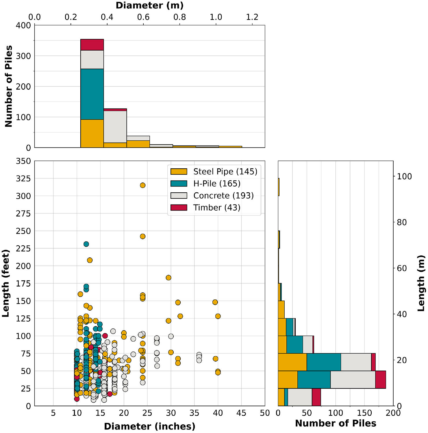
Distribution of piles employed in this study.

The authors aimed to employ as many features as possible in the analysis. Available correlations provided by the Naval Facilities (NAVFAC) Design Manual 7.01 ( 20 ) and Peck et al. ( 21 ) were used to estimate parameters from the available reported parameters. Corrected standard penetration test (SPT) blow count values, denoted as Ncorr, were obtained from the database for each soil stratum. These values were adjusted for overburden pressure effects following Peck et al.’s guidelines. Using these corrected N-values, the authors were able to estimate the soil’s total unit weight according to Bowles’ correlations ( 22 ). In cases where the Ncorr was not directly available, but the layer’s unconfined compressive strength was known, Ncorr was inferred based on NAVFAC’s recommendations. Conversely, the unconfined compressive strength could also be derived from Ncorr when necessary. Finally, q, was determined with the aid of the Robertson zones chart ( 23 ). More details are available in Rizk et al. ( 24 ).

Methods Under Consideration

Traditional Mechanics-Based Design Methods

The performance of four traditional design methods was investigated using the current dataset to provide a baseline for evaluating the efficacy of ML methods. The four chosen methods were selected for use owing to their popularity and availability in APILE software. All methods rely on the same framework consisting of two separate calculations for toe resistance, R_p, and shaft resistance, R_s, and their summation is the ultimate bearing capacity, Q_c. Detailed descriptions of the methods are available in Reese et al. ( 14 ), Hannigan et al. ( 15 ), and Wang et al. ( 19 ). The selected design methods were

• FHWA: The method calculates the capacity in cohesionless soils using Nordlund’s method ( 25 ) and cohesive soils with Tomlinson’s method ( 26 ). The method contains several charts to account for different effects and can be considered the most complex among the traditional methods.

• USACE: The fundamental property of USACE ( 16 ) is its use of the critical depth concept (D_c), which limits the unit skin friction and bearing resistance after a certain depth depending on the pile diameter and the relative density of sand. USACE uses Tomlinson’s method for cohesive soils.

• API: This design method ( 17 ) relies mainly on visual descriptions of cohesionless soils and employs a table that correlates design parameters to relative density and soil description. Notably, API adopts limiting skin friction and end bearing values for cohesionless soils. For cohesive soils API employs an adhesion factor (α-coefficient) that differs somewhat from other methods.

• Revised lambda: The model computes skin friction in cohesive soils. The method is unique in that it accounts for relative pile stiffness as well as decreases in overconsolidation and load transfer with depth. APILE converts cohesionless layers to an equivalent cohesive layer and calculates the skin friction accordingly. For end bearing in any soil, APILE also employs the API method.

Machine Learning Methods

ML models can be broadly classified as either classification models or regression models. Computation of pile capacity can be viewed as an ML regression model that relies on several features such as pile diameter and length, predominant soil type, or penetration resistance (N-value). Therefore, the first step is to identify the optimal feature set. To do so, several feature selection techniques are available. We used six feature selection techniques and the best performing set from each technique was used for model training. In parallel, it is also necessary to optimize the hyperparameters for each of the ML models employed. Finally, each of the optimized models was then trained using six feature sets (16 models × 6 feature sets = 96 models). The performance of each of the 16 ML models with the best performing feature subset was employed for further investigations. All ML-related analyses were carried out primarily in the scikit-learn package ( 27 ) with XGBOOST ( 28 ) and LightGBM ( 29 ) packages employed where needed.

Feature Selection Methodology

Feature selection is a common practice employed in ML to select the most correlated and informative features from a dataset that would allow the model to predict or classify the target variable. Features for model training might include pile (1) type, (2) material, (3) diameter, (4) length, (5) area, (6) circumference, (7) modulus of elasticity, and average (8) total unit weight of soil, (9) N-value, (10) undrained shear strength ( $S_{u})$ , (11) internal friction angle (φ), (12) cone penetration testing’s cone tip resistance, q_c, along the pile, and (13) predominant soil type, among others. Some of these features are correlated with each other whereas other features may not be correlated with capacity. Thus, using all features can lead to poor model performance. To enhance the accuracy of the models, six different feature selection techniques were investigated. The first was the variance threshold model, which removes the features with a variance lower than a predefined threshold. This threshold should be defined considering the nature of the problem and feature set. A threshold of 100 was selected after visually inspecting the variance plot of each feature. The second technique was the SelectKBest method, which is a method that ranks the features depending on a statistical test and selects the top-performing “k” number of features. The analysis used f_regression as the statistical test among the available tests since the task was a regression task. F-score is a measure of how strong the relationship between a feature and the target variable is and how statistically significant the relationship is. A k number of four was selected since scores for k > 4 were close to zero. The third method employed in this study was recursive feature elimination cross-validation (RFECV), which relies on a routine that starts with training a model with the most comprehensive feature set and removing the least important feature in every step until the underlying model suffers as a result of the removal of a feature. The fourth method was tree-based feature selection, which is also based on the calculation of feature importance considering the impurity of the tree nodes. Feature importance for this method is calculated by considering the calculated impurity for each feature, and the technique eliminates the features below a certain threshold. L1-based feature selection, also known as LASSO (least absolute shrinkage and selection operator), was the fifth method used in the analysis. This technique takes the absolute coefficients from the underlying model and eliminates the features with a smaller coefficient than its threshold. Both tree-based feature selection and L1-based feature selection employed the mean feature importance as their threshold for selecting features. Lastly, the sequential feature selection method was employed. This method can go forward starting from an empty feature set and adding the most important feature, or be backward starting with a complete feature set and deleting the least important feature at each step until a predefined number of features is reached or the addition or deletion of a feature does not increase the model score anymore. A detailed description of the aforementioned feature selection methodologies is provided by Ozturk et al. ( 30 ).

Hyperparameter Optimization

The feature selection methods were followed by employing a hyperparameter optimization method called RandomSearchCV, which randomly samples the hyperparameters from a predefined hyperparameter pool and evaluates the model’s performance using a scoring metric to find the optimal hyperparameters for the model ( 31 ). The mean absolute percentage error (MAPE) was used in this study as a scoring metric since MAPE is deemed to be the most important accuracy indicator for axial pile capacity ( 32 ). In scikit-learn, scoring functions are designed such that higher scores indicate better performance. Consequently, to align with this framework, the negative of the MAPE was utilized. The MAPE metric is normally a measure of loss indicating a lower score is better. However, this was negated so that a higher value became better, to comply with scikit-learn’s scoring approach. The hyperparameter optimization involved training 32,000 different models (16 models × 400 trials × 5 cross-validations) to get the best hyperparameters for a given model. The selection of 32,000 models for hyperparameter tuning was driven by the aim to conduct a thorough and comprehensive exploration of the hyperparameter space. This extensive number of trials was chosen after several iterations of trial and error, during which the authors assessed the adequacy of different trial counts. It was determined that this specific number of trials was sufficient to reliably identify the best performing models. This approach reflects a balance between thoroughness in hyperparameter exploration and practical considerations of computational resources and time. The RandomSearchCV method also employs cross-validation technique that involves splitting the dataset into multiple subsets, referred to as folds, and training each fold separately in an effort to prevent overfitting.

ML Models

Sixteen different ML algorithms were explored, and their performance with the features identified by the previously mentioned six feature selection methods were evaluated (96 models). Nine out of 16 ML algorithms could be considered base ML algorithms, whereas seven were classified as ensembles of the base algorithms.

A linear regression model can be mathematically expressed as $\hat{y}$ =β₀+β₁·X₁+β₂·X₂+…+β_n·X_n, where β₀ is the intercept, and β₁ through β_n are linear coefficients with each feature X. Linear models typically aim to minimize a cost function, known as the ordinary least squares loss function,

Cos t_{linear} = \frac{1}{2 n} \sum_{i = 1}^{n} {(y_{i} - {\hat{y}}_{i})}^{2}

(1)

where

n is number of samples,

$y_{i}$ is actual value of target for the ith sample, and

${\hat{y}}_{i}$ is predicted value using linear regression equation.

Linear regression-based ML models are based on the same principle, with additional considerations of the cost function.

The following linear-based ML models were employed in this study. Detailed descriptions of the models are available in Ozturk et al. ( 32 , 33 ). The following is a brief summary:

○ Ridge regression is a linear regression with L2 regularization ( 34 ). A regularization usually introduces penalty terms to the linear coefficients. L2 regularization tries to shrink all coefficients toward zero without eliminating any of them, since it assigns a penalty term proportional to the square of the coefficients. The cost function for ridge regression is provided below, where $λ$ is the regularization parameter, and p is the number of features.

Cos t_{Ridge} = \frac{1}{2 n} \sum_{i = 1}^{n} {(y_{i} - {\hat{y}}_{i})}^{2} + λ \sum_{j = 1}^{p} β_{j}^{2}

(2)

○ Bayesian ridge regression treats the penalty term as a random variable and employs Bayes’ theorem for updating it with iterations.

○ LASSO regression is another linear regression with LASSO (L1) regularization that can eliminate features by assigning penalty terms proportional to the model’s coefficients ( 35 ). As the regularization parameter becomes stronger, the contribution of the prediction error to the cost function becomes smaller compared with the penalty. LASSO can eventually force $β_{j}$ to become exactly zero owing to the discontinuous shape of the cost function around zero with sharp change in the slope of $β_{j}$ . The abrupt change in the value and behavior of the cost function around zero causes the optimization algorithm to favor parameters that result in exactly zero for some coefficients, effectively eliminating the feature from the model.

Cos t_{Lasso} = \frac{1}{2 n} \sum_{i = 1}^{n} {(y_{i} - {\hat{y}}_{i})}^{2} + λ \sum_{j = 1}^{p} | β_{j} |

(3)

○ ElasticNet regression employs both ridge and LASSO regularizations simultaneously ( 36 ). It is deemed especially useful when there are multiple correlated features.

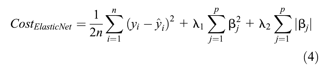
Cos t_{ElasticNet} = \frac{1}{2 n} \sum_{i = 1}^{n} {(y_{i} - {\hat{y}}_{i})}^{2} + λ_{1} \sum_{j = 1}^{p} β_{j}^{2} + λ_{2} \sum_{j = 1}^{p} | β_{j} |

(4)

The following nonlinear models were also used:

• Stochastic gradient descent (SGD) regression ( 37 ) is a regression algorithm that uses gradient descent optimization for minimizing the cost function. Linear models typically employ coordinate descent optimization, in which the algorithm updates one parameter at a time while holding the others fixed. Gradient descent aims to find the steepest descent, meaning the one that minimizes the cost function most in the entire parameter space and updates all parameters simultaneously. SGD iteratively updates model coefficients by processing small random subsets of data at a time and moving in the direction of the negative gradient of the cost function until the convergence criteria is met.

• Kernel ridge regression (KRR) ( 38 ) combines ridge regression with a so-called “kernel trick” that allows the higher-dimensional mapping that involves applying a kernel function to transform data from a lower-dimensional space to a higher-dimensional space. This mapping is implicit and is used to capture complex relationships and patterns that might not be obvious in the original data space. By calculating inner products in this higher-dimensional space, ML algorithms can effectively work with nonlinear relationships and make accurate predictions. There are three common kernel functions. The linear kernel provides no transformation whereas the polynomial kernel works with the inner products between two points in a high-dimensional space to map polynomial combinations. Lastly, the radial basis function or Gaussian kernel measures the similarity between points as a Gaussian (bell-shaped) function of the Euclidean distance between them.

• Support vector regression (SVR) ( 39 ). Support vector machines’ objective is to find a hyperplane that separates the classes using nearby data points known as support vectors. SVR finds the flattest tube that contains most of the training dataset. It employs a similar kernel trick to that used in KRR to handle both linear and nonlinear relationships, aiming to find the tube that best fits the data within a margin.

• k -nearest neighbor (kNN) regression predicts the target variable by taking the average of the k-nearest points. The nearest neighbor points are determined based on the proximity between the points measured as a euclidean distance. For every new input, the model finds the k-nearest points in the training set on a feature plane and takes the average of those instances ( 40 ).

• Decision tree regression relies on partitioning the data and sample space, and the prediction is the mean of a particular group ( 41 ). In each step of the partitioning process, the test is selected in such a way as to minimize the loss function, which is usually the mean squared error. It splits the data into subsets based on feature values and navigates in the tree-like structure from root to leaf to find the group of the new input.

Ensemble models typically combine multiple iterations of the same base model, however algorithms combining multiple linear or nonlinear models have also been reported ( 42 , 43 ). The following ensemble ML models were explored, all of which combined repeated runs of the same base models:

• Bagging decision trees: Bagging involves training multiple models with subsets from the same dataset. All data can be sampled for each new subset ( 44 ). In this case, multiple decision trees were trained, and the final prediction is the average of all trained trees.

• Random forest: Random forest employs the bagging technique with decision trees as well. However, random forest goes one step further by using random subsets of the available features.

• Extra (extremely randomized) trees: This is a model based on the same principles as the random forest model. The difference is that instead of trying to find the most discriminative split, it randomly splits each node with different values, and it keeps the split that gives the best result.

• Gradient boosting: A boosting method ( 45 ) that trains different models sequentially, and after each trial it either adjusts the weights of high error predictions to minimize the overall training error or, instead of assigning weights, it trains another model using the dataset contributing to high error, which effectively minimizes the overall error of the model. Boosting thus simply aims to learn from the mistakes of previous models. Gradient boosting uses the gradient descent method to minimize the error.

• Extreme gradient boosting (XGBoost) ( 28 ): This is an optimized version of gradient boosting that employs second-order gradients along with regularization to perform better.

• Light gradient boosting (LightGBM): The previous two boosting methods employed used decision trees with a levelwise growth, meaning each node is split to a finite number of branches. In LightGBM ( 29 ) growth always splits the leaf that minimizes the loss first, so trees can grow unbalanced.

• Adaptive boosting (AdaBoost): This method offers a similar framework to gradient boosting, however, it assigns weights to each datapoint ( 46 ). Points that are misclassified get higher weights for the next learner, which aims to minimize the loss function.

Analysis Methodology

The analysis in this study can be divided into several phases. In the first phase, pile capacities were calculated using the traditional design methods and their performance was analyzed (Figure 2). To complete this task, APILE software was used to calculate the capacity from each design method. This process was automated with the help of Python scripts developed by the authors. The first script collected the soil profiles and pile properties that were available in the databases, which were used to create APILE data files. After running each analysis, the output files created by the software were stored, and the results for each method were scraped from those output files and stored in spreadsheets using another Python script.

Figure 2.

Flowchart outlining the methodology.

The calculated capacities (Q_c) were next compared with the measured capacities (Q_m) from the static load tests interpreted using the original Davisson criterion and stored in the databases. The performance of each technique was evaluated by considering the coefficient of determination ( $R^{2}$ ), the average and standard deviation of the normalized capacities (Q_c/Q_m), the mean absolute error (MAE), and MAPE. The coefficient of determination, $R^{2}$ , is considered better as it approaches 1. The mean Q_c/Q_m is expected to be 1: values less than 1 suggests the method’s tendency to underestimate capacity, and values larger than 1 suggests overestimating. The standard deviation of Q_c/Q_m is a measure of precision, giving information about the scatter in computed capacities. MAE measures the average error, whereas MAPE presents the average relative error, making it a feasible metric for comparing methods in relation to accuracy. In contrast to average Q_c/Q_m, MAPE is an absolute metric, therefore two values cannot cancel each other out, however, average Q_c/Q_m can hide defects. For instance, if two Q_c/Q_m values were reported as 0.8 and 1.2, their average would be 1, suggesting perfect accuracy; however, MAPE would suggest that the average error is 20%. The effect of a change in diameter, length, or soil types was also investigated to measure the methods’ consistency.

The second phase of this study involved evaluating the different feature selection techniques to determine the input features that should be used in training the ML methods. The features used in the analysis were the pile’s diameter, length, circumference, area, modulus of elasticity, pile material, and pile type, as well as the average undrained shear strength, cone tip resistance (q_c), SPT blow count (N), angle of internal friction (ϕ), total unit weight, and predominant soil type. These features were used to feed the six different feature selection techniques to determine their recommended subset of features. These techniques were selected in part considering their availability in the commonly used ML libraries.

The third phase in the analysis was hyperparameter optimization of the selected ML methods. Previous studies employed similar models ( 32 , 33 ) but they were used either in their default mode or by manual trial and error for hyperparameter optimization. In this study, a substantial hyperparameter grid for all the models employed was created. The random search optimization technique was employed by conducting 400 trials with fivefold cross-validations, which resulted in each model being trained 2,000 times. Consequently, 32,000 models were trained in this study (16 models × 2,000 iterations = 32,000) with a different subset of the training dataset or different hyperparameters, and the best performers were selected as the tuned models. Optimization was done using the most comprehensive feature set. Ideally, a comprehensive grid search would evaluate every possible combination out of the predefined hyperparameter grid for each subset of features that was selected in the feature selection phase. However, time and resource constraints prevented use of a grid search.

In the final phase, each optimized ML model was trained with six different subsets of features selected during the feature selection techniques phase, which resulted in six different ML models. In total, 96 different models (6 × 16) were trained, and their performance was evaluated considering their test results over the mean and standard deviation of Q_c/Q_m and MAPE. Each model’s best performing feature subset was chosen, and a plot was created for the predicted capacities versus the measured capacities for visual inspection. Finally, the top three models were chosen to compare their performance with the best traditional design method with respect to the effect of change in diameter, length, or soil type on Q_c/Q_m.

Performance of Traditional Design Methods

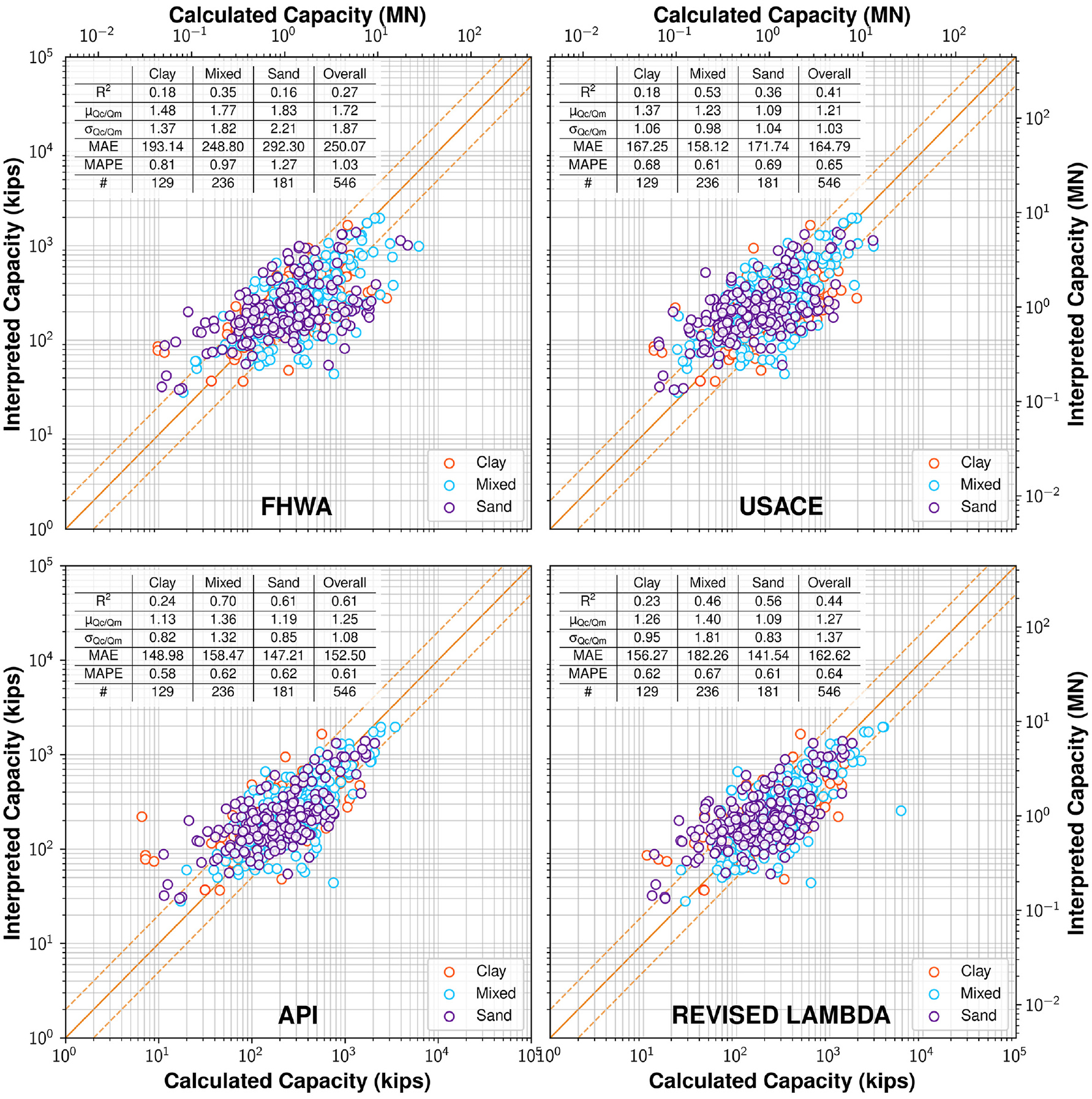
Calculated capacities (Q_c) are plotted against the measured capacities (Q_m) for all four traditional design methods in Figure 3. A solid diagonal line representing the 1:1 relation between Q_c and Q_m is depicted on the figure, while the two dashed parallel lines represent the 1:2 and the 2:1 relationships, respectively. Statistical measures including coefficient of determination ( $R^{2}$ ), mean Q_c/Q_m, standard deviation of Q_c/Q_m, MAE, and MAPE are reported in inset tables embedded in each plot. Each table presents those metrics for each predominant soil type, to facilitate comparison of method performance for each soil type.

Figure 3.

Performance of traditional methods with soil types.

It is difficult to distinguish the best performing method owing to various methods excelling when evaluated by different metrics. It can be observed that the API design method had the best overall MAPE, but revised lambda and USACE also achieved comparable performances. On the other hand, the MAPE of FHWA was considerably worse than the other three methods. In relation to the mean and standard deviation of Q_c/Q_m, USACE performed best with API and revised lambda again being close enough. Finally, API was deemed the best performing method for the dataset at hand owing to its overall accuracy exhibited by the lowest MAPE, MAE, and high precision having one of the lowest standard deviations and highest $R^{2}$ .

In predominantly clayey soils, API had the lowest MAPE, best average, and standard deviation of Q_c/Q_m, whereas USACE and API had the lowest MAPE in mixed soils: 0.61 and 0.62, respectively. However, for the average and standard deviation of Q_c/Q_m, USACE was the best overall design method in clay.

For predominantly sandy soils, the revised lambda and API methods had the best MAPE at 0.61 and 0.62, respectively. Revised lambda had the best average Q_c/Q_m along with USACE. At the same time, standard deviations of revised lambda and API were very close once again, making revised lambda preferable for use in sandy soils. It is noteworthy that revised lambda is intended primarily for clayey soils, and the APILE implementation of the method involves converting sands to clays having a similar shear strength. Therefore, API would be superior in cases in which APILE is not used for computing the capacity in sand.

Next, the effect of change in diameter over the performance of the methods was evaluated. Pile diameter was plotted versus Q_c/Q_m for each design method presented in Figure 4, along with the best fit line, and the slope of the line was also calculated. This time, FHWA showed the lowest change in performance, with diameter, followed by API, and the slopes of the other two methods were very close, being the most affected. The slope of 0.008/in. exhibited by USACE and revised lambda translated to a 9.6% additional overestimation per 12-in. increase in diameter.

Figure 4.

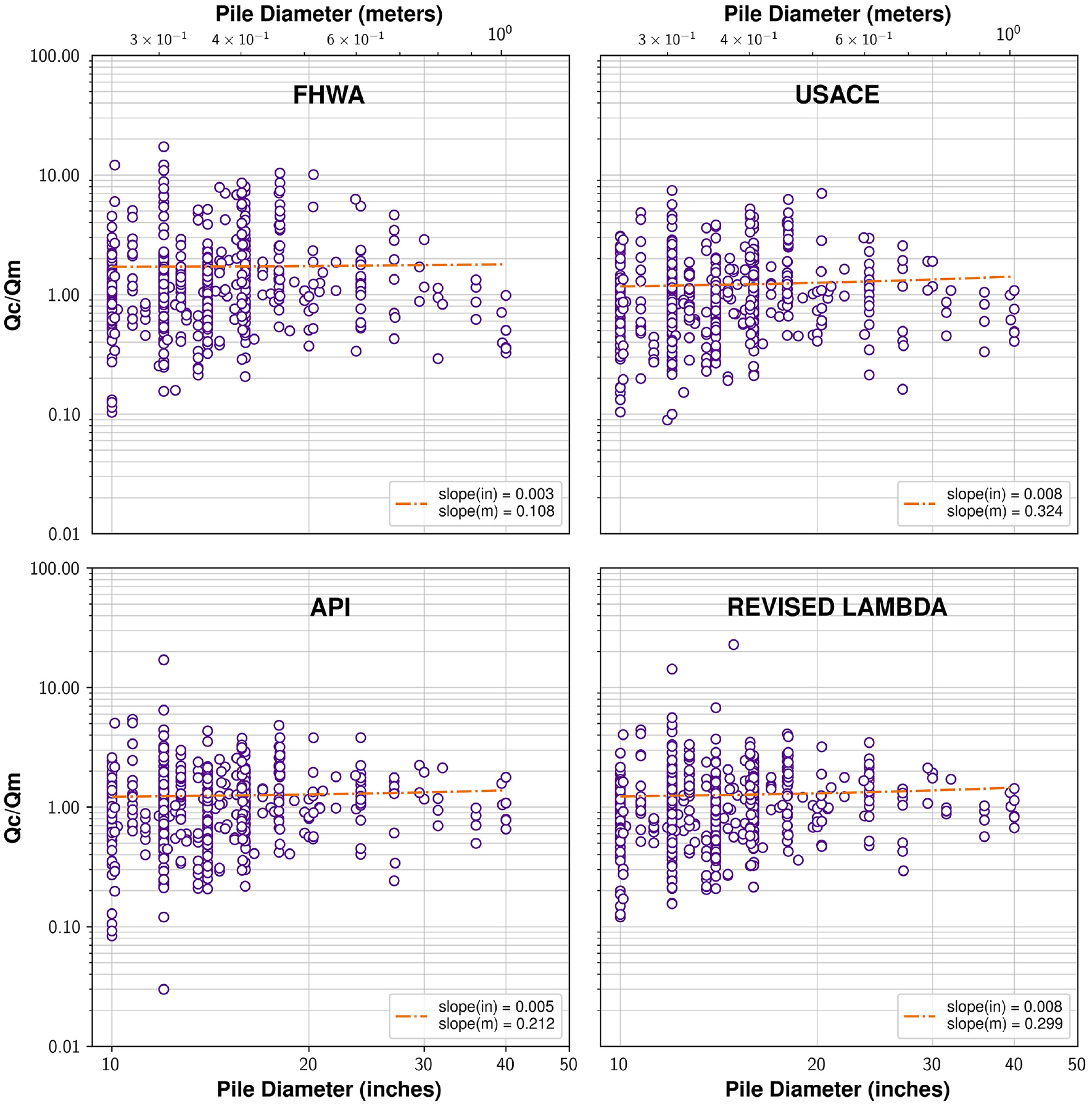
Effect of change in pile diameter on the performance of traditional methods.

Finally, the length effect on the traditional methods was investigated in Figure 5. USACE, exhibited little length effect, with near ideal performance in this case. Considering purely the slope of the fitted line, FHWA was better than the other two methods. API and revised lambda performed worse than the other two methods. For example, revised lambda had a 0.010 slope with increased pile length corresponding to a 10% additional overestimation for every 10-ft increase in length.

Figure 5.

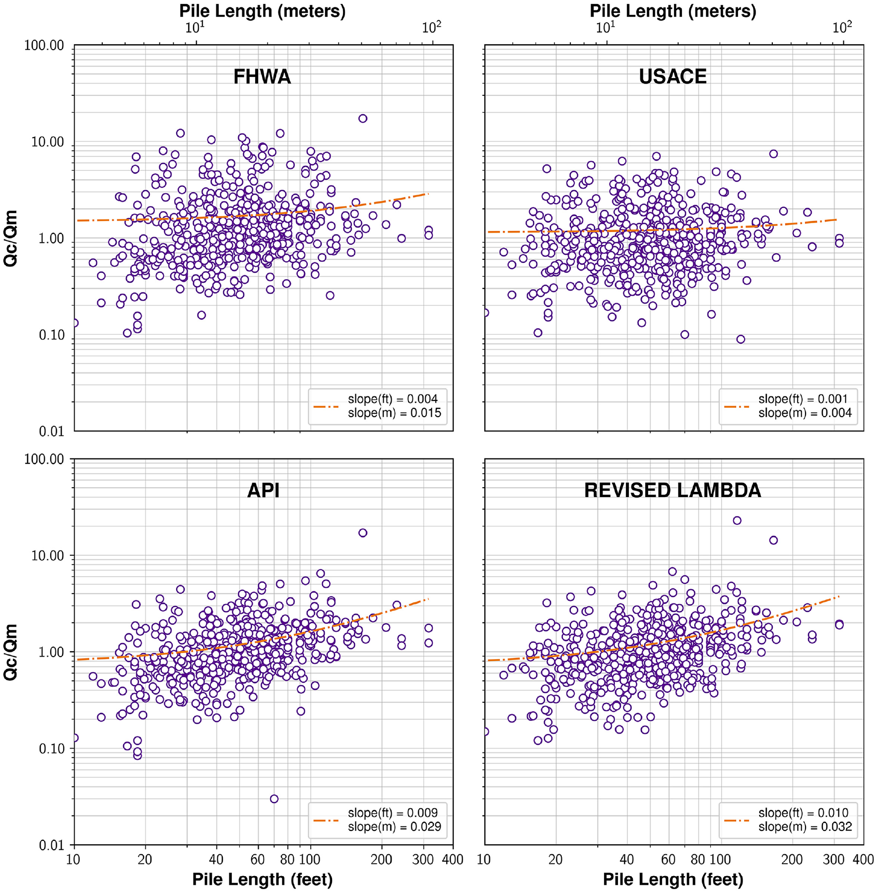
Effect of change in pile length on the performance of traditional methods.

Considering all the preceding factors, API was selected as the baseline method for comparison with the ML models since it provided consistently good performance among all soil types, the best performance in clays, and low influence of change in pile diameter on the predicted capacity. USACE was a close second, whereas FHWA was the worst among the considered methods.

Performance of Machine Learning Methods

Feature Selection Results

After establishing the baseline performance of the traditional methods for the available dataset, the study focused on checking the efficacy of the ML methods to predict the load bearing capacity of a pile. The features employed by a model are essential to train it. Thus, the first step in creating such models was finding the most informative feature set. For that reason, six different commonly used feature selection techniques were employed to identify six different subsets of features. The results of the feature selection techniques are presented in Figure 6, where the length of each bar corresponds to the importance of the feature, except in the case of RFECV, where the methods yield a rank. Solid yellow bars correspond to each technique’s identified features, while the hashed red bars (or no bars) represent features that were not deemed useful by the technique. The following features were selected by each of the selection methods:

• Variance threshold: modulus, area, q_c, length, circumference, N, total unit weight;

• SelectKBest: diameter, length, circumference, area;

• RFECV: pile material, diameter, length, area, circumference, predominant soil type, total unit weight, N, S_u, phi, q_c;

• Tree-based: diameter, length;

• L1-based: length, diameter, S_u; and

• Sequential feature selection: phi, S_u, total unit weight, circumference, length, diameter.

Features varied based on the technique employed to identify them. Some parameters were commonly identified by most selection techniques, whereas others were surprisingly not identified. It is not surprising that nearly all feature selection techniques identified length and diameter among their inputs. In fact, the lowest number of selected features was two, with tree-based feature selection keeping only diameter and length. However, the variance threshold method employed both circumference and area simultaneously rather than the diameter. It is noteworthy that the variance threshold technique only considers the feature’s variance whereas other techniques are based on training performance. Surprisingly, tree-based feature selection and SelectKBest methods did not select any soil-related features. The highest number of features was chosen by RFECV with the method eliminating only pile type and modulus of elasticity, keeping 11 features to be used in the models. Finally, it is noteworthy that the k in the SelectKBest method, is a user input, however, the authors opted to keep the top four features only, considering the massive gap between the score of the fourth and fifth features.

Figure 6.

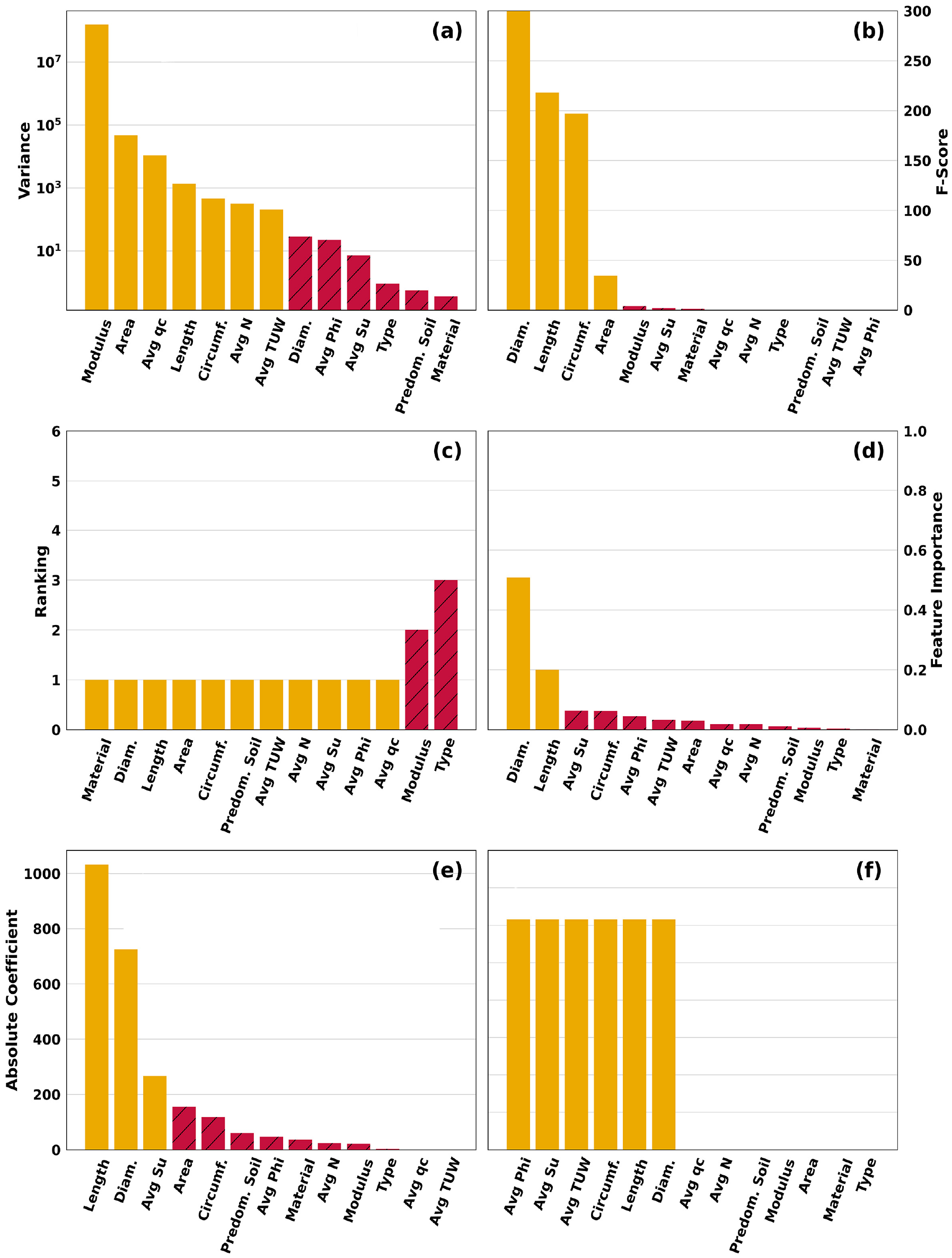
Results of feature selection techniques: (a) VarianceThreshold Feature Selection, (b) SelectKBest Feature Selection with f_regression, (c) RFECV Feature Ranking, (d) Tree-Based Feature Selection, (e) L1-Based Feature Selection and (f) Forward Sequential Feature Selector.

The ubiquity of length and diameter identified by most feature selection methods is consistent with the mechanics-based design practice. However, the lack of soil-related features by several of the methods reflects poorly on the quality of the available soil data and the manner in which geotechnical parameters are acquired, which is unfortunate.

Performance of Machine Learning Models

Six feature sets were identified in the previous step. In parallel, the hyperparameters were optimized with the most comprehensive feature set. Next, all 16 models were trained with six feature sets, and their testing and training performances are reported in Tables 1 and 2, respectively. The performance metrics for evaluation were again the average and standard deviation of Q_c/Q_m and MAPE. The best performing feature set for each model is presented in boldface in Table 2 and also plotted in Figures 7 and 8 along with the baseline performance from the traditional techniques, that is, the API method, allowing for visual inspection of the results.

Table 1.

Training Performance of Machine Learning Models Using the Subset of Respective Feature Selection Method

Models	Variance threshold			SelectKBest			RFECV			Tree-based feature selection			LASSO-based feature selection			Sequential feature selection
Models	$μ$ ^†	$σ$ ^‡	MAPE	$μ$	$σ$	MAPE	$μ$	$σ$	MAPE	$μ$	$σ$	MAPE	$μ$	$σ$	MAPE	$μ$	$σ$	MAPE
Random forest	1.16	0.57	0.27	1.19	0.66	0.34	1.13	0.4	0.24	1.21	0.68	0.38	1.16	0.49	0.29	1.15	0.44	0.26
Extra trees	1.16	0.57	0.28	1.22	0.68	0.37	1.13	0.41	0.23	1.27	0.78	0.45	1.2	0.58	0.35	1.15	0.46	0.27
Gradient boosting	1.08	0.27	0.17	1.16	0.56	0.31	1.06	0.22	0.14	1.23	0.71	0.4	1.12	0.39	0.26	1.08	0.28	0.18
XGBoost	0.79	0.4	0.36	0.82	0.5	0.39	0.78	0.33	0.34	0.9	0.57	0.42	0.83	0.4	0.36	0.78	0.32	0.34
LightGBM	1.08	0.4	0.2	1.19	0.7	0.36	1.06	0.26	0.16	1.22	0.74	0.41	1.12	0.48	0.28	1.08	0.35	0.2
Bagging DT	1.25	0.86	0.42	1.27	0.82	0.45	1.22	0.57	0.37	1.27	0.82	0.47	1.23	0.64	0.4	1.21	0.56	0.37
AdaBoost	1	0.01	0	1.01	0.12	0.03	1	0.01	0	1.02	0.18	0.05	1	0.01	0	1	0.01	0
kNN	1	0.01	0	1.01	0.11	0.02	1	0.01	0	1.02	0.17	0.05	1	0.01	0	1	0.01	0
Decision tree	1.21	1.01	0.5	1.2	0.87	0.5	1.24	0.93	0.55	1.28	1.16	0.58	1.21	1.02	0.53	1.17	0.78	0.47
Ridge regression	1.39	1.04	0.61	1.37	0.99	0.59	1.35	0.9	0.56	1.41	0.98	0.61	1.4	0.95	0.6	1.36	0.95	0.57
SGD	1.07	0.75	0.48	0.87	0.7	0.49	1.09	0.72	0.47	0.59	0.44	0.51	0.92	0.62	0.45	1.09	0.73	0.47
LASSO	1.24	1.03	0.57	1.14	0.87	0.49	1.2	0.88	0.5	1.1	0.82	0.48	1.16	0.82	0.48	1.17	0.88	0.5
ElasticNet	0.51	0.45	0.6	0.16	0.13	0.84	0.64	0.52	0.54	0.08	0.06	0.92	0.16	0.11	0.84	0.33	0.22	0.69
Bayesian ridge	1.35	1.14	0.62	1.29	0.98	0.56	1.27	0.92	0.52	1.27	0.96	0.55	1.35	0.95	0.57	1.3	0.96	0.56
Kernel ridge	1.29	0.92	0.5	1.32	0.89	0.53	1.22	0.77	0.44	1.33	0.88	0.54	1.27	0.77	0.49	1.25	0.76	0.46
SVR	1.16	0.86	0.44	1.15	0.77	0.44	1.12	0.68	0.35	1.2	0.84	0.48	1.14	0.69	0.41	1.11	0.58	0.35

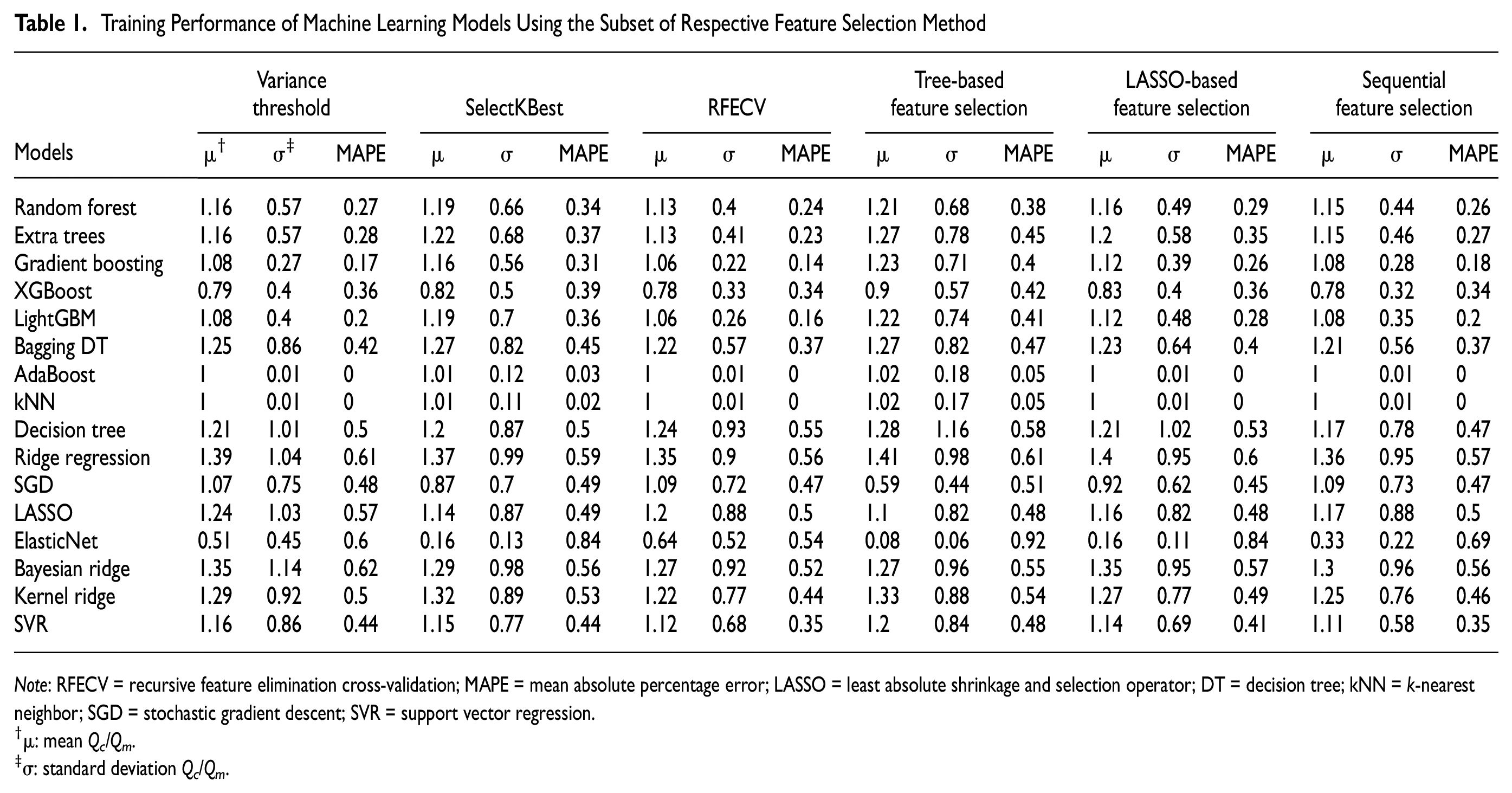
Note: RFECV = recursive feature elimination cross-validation; MAPE = mean absolute percentage error; LASSO = least absolute shrinkage and selection operator; DT = decision tree; kNN = k-nearest neighbor; SGD = stochastic gradient descent; SVR = support vector regression.

†

$μ$ : mean Q_c/Q_m.

‡

$σ$ : standard deviation Q_c/Q_m.

Table 2.

Testing Performance of Machine Learning Models Using the Subset of Respective Feature Selection Method

Models	Variance threshold			SelectKBest			RFECV			Tree-based feature selection			LASSO-based feature selection			Sequential feature selection
Models	$μ$ ^†	$σ$ ^‡	MAPE*	$μ$	$σ$	MAPE	$μ$	$σ$	MAPE	$μ$	$σ$	MAPE	$μ$	$σ$	MAPE	$μ$	$σ$	MAPE
Random forest	1.3	0.76	0.49	1.35	0.81	0.55	1.31	0.7	0.48	1.41	1.04	0.65	1.31	0.78	0.54	1.33	0.74	0.5
Extra trees	1.32	0.8	0.49	1.37	0.88	0.56	1.32	0.74	0.49	1.42	0.98	0.63	1.32	0.79	0.53	1.35	0.78	0.52
Gradient boosting	1.27	0.94	0.46	1.35	1.01	0.58	1.3	0.87	0.48	1.38	1.01	0.64	1.28	0.83	0.52	1.28	0.83	0.51
XGBoost	0.85	0.5	0.37	0.9	0.59	0.43	0.87	0.53	0.38	0.98	0.71	0.47	0.88	0.53	0.39	0.87	0.52	0.38
LightGBM	1.29	0.93	0.5	1.3	0.93	0.55	1.23	0.76	0.49	1.34	1.06	0.62	1.22	0.78	0.54	1.23	0.81	0.52
Bagging DT	1.33	0.8	0.52	1.37	0.85	0.58	1.33	0.72	0.51	1.37	0.9	0.6	1.31	0.77	0.53	1.33	0.75	0.52
AdaBoost	1.18	0.71	0.42	1.28	0.8	0.52	1.19	0.6	0.42	1.44	1.59	0.73	1.2	0.76	0.48	1.21	0.65	0.45
kNN	1.31	0.94	0.52	1.28	0.85	0.5	1.3	0.86	0.52	1.44	1.39	0.66	1.26	0.73	0.51	1.3	0.82	0.5
Decision tree	1.22	0.83	0.54	1.28	0.91	0.56	1.31	0.92	0.59	1.32	1.06	0.62	1.28	0.88	0.58	1.27	0.78	0.55
Ridge regression	1.49	1.15	0.71	1.47	1.01	0.68	1.45	0.96	0.65	1.5	0.99	0.69	1.47	0.94	0.67	1.45	0.97	0.66
SGD	1.15	0.86	0.5	0.94	0.74	0.51	1.17	0.75	0.47	0.63	0.46	0.52	0.89	0.5	0.4	1.14	0.69	0.45
LASSO	1.37	1.17	0.67	1.22	0.91	0.59	1.29	0.91	0.59	1.16	0.85	0.56	1.21	0.82	0.55	1.24	0.9	0.58
ElasticNet	0.56	0.59	0.63	0.18	0.14	0.83	0.66	0.53	0.52	0.09	0.07	0.91	0.15	0.09	0.85	0.34	0.2	0.67
Bayesian ridge	1.42	1.14	0.7	1.37	1	0.66	1.3	0.95	0.64	1.34	0.99	0.65	1.4	0.95	0.65	1.34	0.94	0.64
Kernel ridge	1.31	0.81	0.52	1.39	0.92	0.6	1.24	0.72	0.49	1.4	0.91	0.62	1.29	0.73	0.53	1.29	0.72	0.51
SVR	1.18	0.75	0.46	1.24	0.86	0.51	1.18	0.64	0.43	1.28	0.88	0.55	1.18	0.68	0.47	1.2	0.67	0.45

†

$μ$ : mean Q_c/Q_m.

‡

$σ$ : standard deviation Q_c/Q_m.

Figure 7.

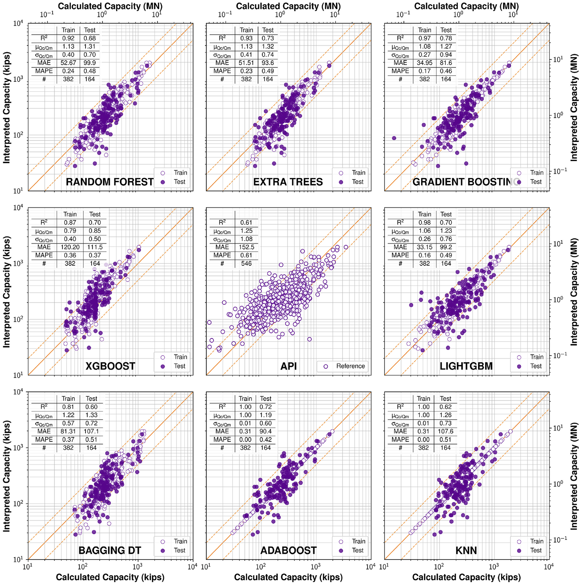
Performance of machine learning (ML) Models 1 to 8, against best traditional method (API). Feature selection method is identified for ML method in inset. Corresponding features are available in Figure 6.

Figure 8.

Performance of machine learning (ML) Models 9 to 16, against best traditional method (API). Feature selection method is identified for ML method in inset. Corresponding features are available in Figure 6.

Ten out of 16 models used RFECV, whereas variance threshold and lasso-based feature selection were used by three models each. The superior performance of the RFECV might have been caused by the method employing the highest number of features. It is noteworthy that some of the models being used here can select their features, so RFECV provided them with more options to choose from. Also, since the models were optimized using all the features, there might be a bias originating from there. A surprising outcome was the performance of LASSO, considering only three features were selected. LASSO was not only the top performer for three methods but was also very close to the top performance in most other methods. This is quite promising, given that the method requires only length, diameter, and undrained shear strength to estimate the capacity of a pile.

The performance of the 16 ML models is depicted in Figures 7 and 8 along with the performance of the API method as a baseline. Although some of the ML models performed well numerically, some apparent flaws were evident when the data were presented graphically. For example, the decision tree and SGD models outperformed API on every metric except coefficient of determination (Figure 8). In the case of the decision tree, it appears that the model acts as a classification model rather than a regression algorithm, as evidenced in the data appearing to be binned. The SGD model appears to have a tendency toward underestimating the capacity with the increase in interpreted capacity. Despite having the second best MAPE after XGBoost, SGD showed that evaluation based on only the statistical measures might be misleading in this topic, and a visualization or a statistical metric that shows how well the results are aligning, such as R², is required for a robust evaluation. A similar concern was also evident for the ElasticNet model, but it also exhibited inferior metrics of average Q_c/Q_m compared with API.

Overfitting was another problem that was visible from Tables 1 and 2. kNN and AdaBoost are clearly overfitting which was evident in their perfect predictions ( $μ ≅ 1, σ ≅ 0, MAPE ≅ 0)$ , suggesting that the models memorized the dataset. The sharp difference in the performance of these models with the testing dataset was consistent with overfitting. Overfitting is generally characterized by a difference between the performance of testing and training sets. Random forest, extra trees, gradient boosting, and LightGBM are also susceptible to overfitting, considering that the MAPEs of the testing sets were double those of the training sets. However, despite some overfitting, random forest, extra trees, gradient boosting, AdaBoost, and LightGBM performed very well, considering their performance with the testing dataset.

MAPE provides an overall measure of accuracy, and when considered alone XGBoost would be the top-performing ML model, followed by SGD, AdaBoost, and SVR. However, Since SGD exhibited an underestimation tendency (Figure 8), the authors decided to keep XGBoost, AdaBoost, and SVR as their top three performing ML models. It is interesting to note that SVR and AdaBoost used the RFECV feature subset, whereas XGBoost used the variance threshold subset.

Several design methods exhibit a length or diameter effect (4 –8). Therefore, the diameter effect of the top three ML models was evaluated along with API. The variation of Q_c/Q_m with respect to pile diameter is presented in Figure 9 on log-linear plots, and the trends are calculated on a linear scale. Although API performed well, AdaBoost performed better, and SVR performed similarly to the API baseline. XGBoost, on the other hand, showed a higher underestimation than API, with the increasing diameter representing approximately an extra 15% underestimation with every 12-in. increase in diameter.

Figure 9.

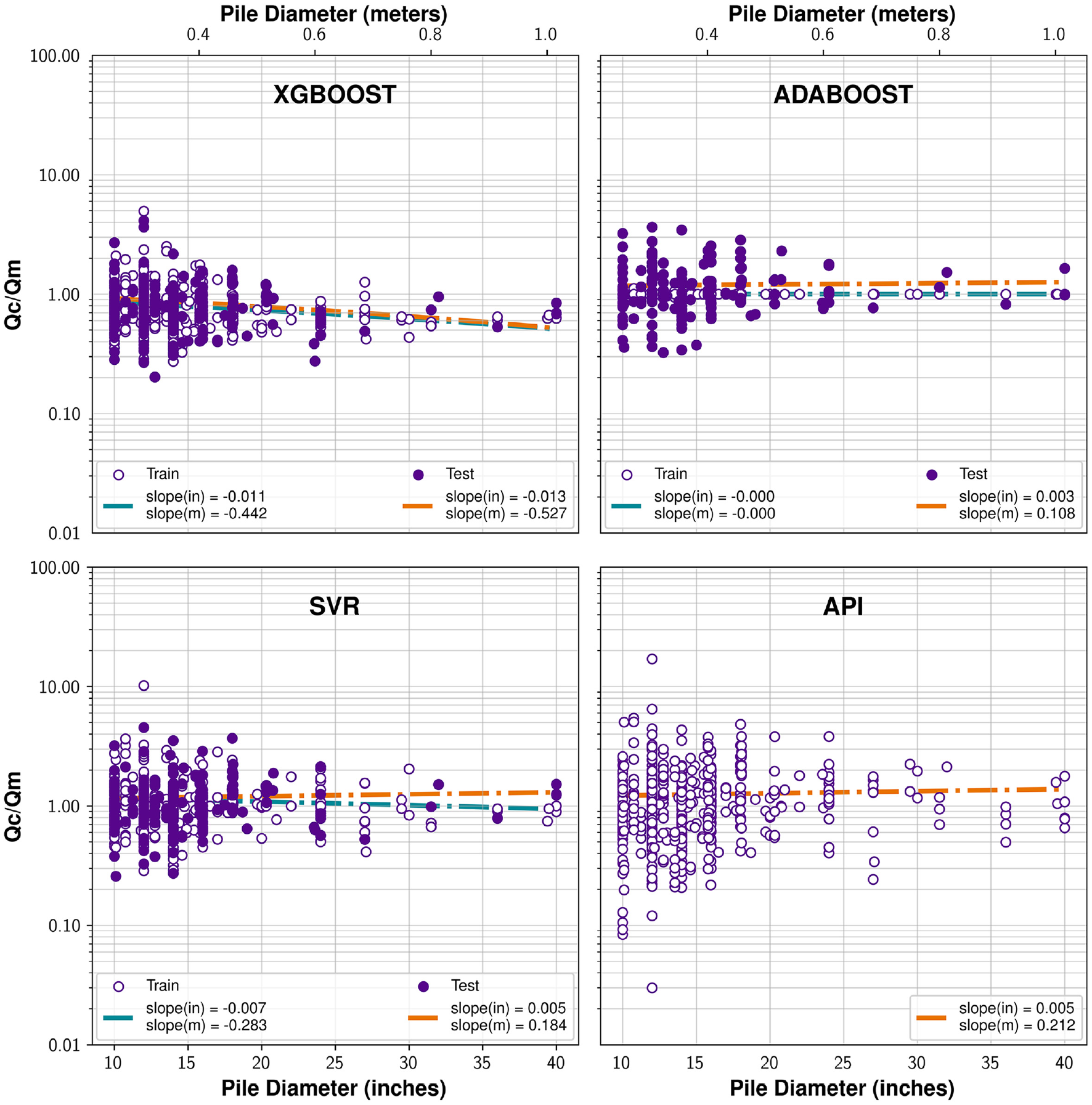
Effect of pile diameter on Q_c/Q_m of the top three machine learning (ML) models and top traditional method (API).

Next, Q_c/Q_m is plotted versus pile length in Figure 10. This time, all three ML models showed almost no vulnerability and outperformed API and other traditional methods in this evaluation.

Figure 10.

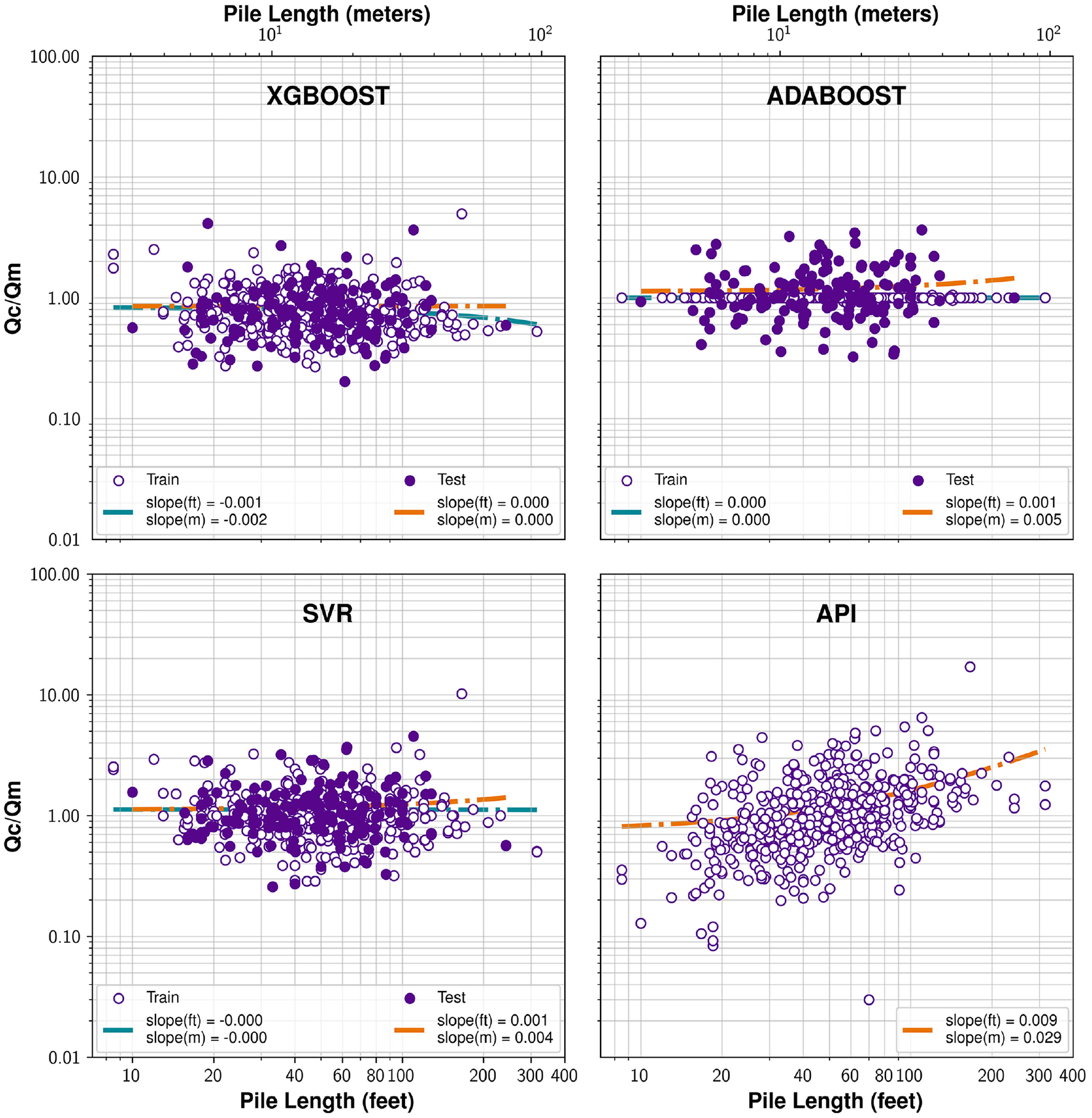
Effect of pile length on $Q_{c} / Q_{m}$ for the top three machine learning (ML) models and API.

Finally, Q_c was plotted against Q_m in Figure 11 for the three top-performing ML models and API, grouped by the predominant soil type. The figures also depict a solid 1:1 line as well as 2:1, and 0.5:1 dashed lines. Only the testing subset is used in Figure 11. None of the four methods was significantly affected by the soil type. A new metric was introduced to better understand the performance, such that the number of poor predictions was counted for each method. Poor prediction is defined as the predictions that are either larger than double or less than half of the interpreted capacity, essentially the number of circles outside the dashed parallel lines to the diagonal. Out of 164 cases, 20, 25, and 31 poor predictions were observed for SVR, AdaBoost, and XGBoost respectively. In comparison, API had 47 poor performing cases, representing 29% of all cases. This percentage was 12% for SVR, 15% for AdaBoost, and 19% for XGBoost. None of the methods were outperformed by API in $R^{2}$ , standard deviation of Q_c/Q_m, or MAPE, indicating the decisive superiority of ML models over the best traditional method. All three ML methods performed reasonably well in nearly all metrics except average Q_c/Q_m, where SVR performed best for sand whereas XGBoost performed best for mixed soils and clays.

Figure 11.

Performance of top three machine learning (ML) models and API, classified by soil type.

Summary and Conclusions

Several ML models were developed to predict the axial load bearing capacity of piles, using a dataset consisting of 546 piles. First, a base line was established by evaluating the accuracy and precision of four traditional mechanics-based design methods. The metrics used for evaluation were the MAPE, as well as the average and standard deviation of the computed normalized by measured capacity (Q_c/Q_m). Second, six feature selection techniques were employed to determine the best feature set to be used for training the ML models. Simultaneously, 16 ML models were optimized by tuning their hyperparameters. Third, all ML models were trained using 70% of the data and with the outputs of six feature selection techniques (96 models), and the best performing feature set was selected for each model. Fourth, The ML models were tested using the remaining 30% of data. Finally, the performance of the ML models was compared with that of the established baseline. The following is a summary of the observations and lessons learned:

• The best performing ML model performed significantly better than the best traditional mechanics-based model, which is encouraging. In particular, the number of cases over- or underestimated by a factor of 2 dropped from 29% to between 12% and 19% for the best three ML models.

• The best performing ML models for the available dataset were SVR, XGBoost, and AdaBoost. SVR performed best for sand whereas XGBoost performed best for mixed soils and clays.

• Ensemble ML models generally performed better than base models, but SVR, which is a base model, performed on par with the ensemble models.

• API performed best among the traditional design methods and was selected as the baseline for comparison. FHWA design method exhibited lower accuracy and precision than the other three traditional methods.

• RFECV was the best performing feature selection method for half of the ML models. It benefited from including nearly all features. Surprisingly, the lasso-based feature selection picked only three features, namely diameter, length, and undrained shear strength, and performed quite well in most of the models, close to the performance of the RFECV, which had 11 features.

The preceding work demonstrates that ML may offer advantages in geotechnical design when large datasets are available. Finally, the authors are of the opinion that the accuracy of the employed ML models could increase tremendously if the available dataset is increased by one to two orders of magnitude.

Footnotes

Acknowledgements

The first author gratefully acknowledges the Fellowship awarded by the Institute of Design and Construction Foundation.

Author Contributions

The authors confirm contribution to the paper as follows: study conception and design: M. Iskander, B. Ozturk, A. Kodsy; data collection: A. Kodsy, B. Ozturk; analysis and interpretation of results: B. Ozturk, M. Iskander; draft manuscript preparation: B. Ozturk. writing – review & editing: M. Iskander. All authors reviewed the results and approved the final version of the manuscript.

Declaration of Conflicting Interests

The authors declared no potential conflicts of interest with respect to the research, authorship, and/or publication of this article.

Funding

The authors received no financial support for the research, authorship, and/or publication of this article.

ORCID iDs

Baturalp Ozturk

Antonio Kodsy

Magued G. Iskander

References

Rizk

Kodsy

Iskander

Machairas

Efficacy of Design Methods for Predicting the Capacity of Large-Diameter Open-Ended Piles. Journal of Geotechnical and Geoenvironmental Engineering, Vol. 148, No. 10, 2022, p. 04022078. https://doi.org/10.1061/(ASCE)GT.1943-5606.0002824.

Machairas

Highley

G. A.

Iskander

M. G.

Evaluation of FHWA Pile Design Method Against the FHWA Deep Foundation Load Test Database Version 2.0. Transportation Research Record: Journal of the Transportation Research Board, 2018. 2672: 268–277.

Ozturk

Kodsy

Bazi

Iskander

Efficacy of Several Design Methods for Predicting the Axial Compressive Capacity of Piles. Transportation Research Record: Journal of the Transportation Research Board, 2023. 2677: 1–17.

Briaud

J. L.

Tucker

L. M.

Measured and Predicted Axial Response of 98 Piles. Journal of Geotechnical Engineering, Vol. 114, No. 9, 1988, pp. 984–1001.

O’Neill

M. W.

Side Resistance in Piles and Drilled Shafts. Journal of Geotechnical and Geoenvironmental Engineering, Vol. 127, No. 1, 2001, pp. 3–16.

Lacasse

Uncertainties in Offshore Geotechnical Engineering, International Survey of API RP2A Design Parameters for Axial Capacity of Driven Piles in Sand. Report No: 85307-14. Norwegian Geotechnical Institute, Oslo, 1988.

Olson

R. E.

Iskander

Axial Load Capacity of Piles in Sand. Proc., Fourth International Conference on Case Histories in Geotechnical Engineering, St. Louis, MO, Missouri University of Science & Technology, 1998, pp. 293–300.

Dennis

N. D.

Olson

R. E.

Axial Capacity of Steel Pipe Piles in Clay. Proc., Conference on Geotechnical Practice on Offshore Engineering, Austin, TX, ASCE, New York, 1983, pp. 370–388.

Dennis

N. D.

Olson

R. E.

Axial Capacity of Steel Pipe Piles in Sand. Proc., Conference on Geotechnical Practice on Offshore Engineering, Austin, TX, ASCE, New York, 1983, pp. 389–402.

10.

Olson

Iskander

Axial Load Capacity of Pipe Piles in Sands. In From Soil Behavior Fundamentals to Innovations in Geotechnical Engineering (R. E. Olson, ed.), GSP No. 233. ASCE Press, New York, 2014, pp. 209–220. https://doi.org/10.1061/9780784413265.

11.

Petek

Mitchell

Ellis

FHWA Deep Foundation Load Test Database VERSION 2.0 User Manual. Report No. FHWA-HRT-17-034. Federal Highway Administration, McLean, VA, 2016.

12.

Roling

M. J.

Sritharan

Suleiman

M.T.

Development of LRFD Procedures for Bridge Piles In Iowa Volume I: An Electronic Database For Pile Load Tests (PILOT). Report No. IHRB Project TR-573, 2011. https://intrans.iastate.edu/app/uploads/2018/03/tr-573_lrfd_vol_1_w_cvr.pdf.

13.

Kodsy

Iskander

Sampurnanand

A. P.

Universal Criterion for Interpreting Capacity from Load Tests on Piles. Transportation Research Record: Journal of the Transportation Research Board, 2022. 2676: 530–541.

14.

Reese

L. C.

Isenhower

W. M.

Wang

S. T.

Analysis and Design of Shallow and Deep Foundations. John Wiley & Sons, Hoboken, NJ, 2005.

15.

Hannigan

P. J.

Rausche

Likins

G. E.

Robinson

B. R.

Becker

M. L.

Design and Construction of Driven Pile Foundations – Volume 1. Report No. FHWA-NHI-16-009. National Highway Institute, U.S. Department of Transportation, Federal Highway Administration, Washington, D.C., 2016.

16.

U.S. Army Corps of Engineers (USACE). Design of Pile Foundations. Engineer Manual 1110-2-2906. U.S. Army Corps of Engineers, Washington, D.C., 1991.

17.

American Petroleum Institute (API). API Recommended Practice for Planning, Designing, and Constructing Fixed Offshore Platforms. Report RP-2A. American Petroleum Institute, Production Department, Washington, D.C., 1993.

18.

Kraft

L. M.

Jr. Focht

J. A.

Jr. Amerasinghe

S. F.

Friction Capacity of Piles Driven into Clay. Journal of the Geotechnical Engineering Division, Vol. 107, No. 11, 1981, pp. 1521–1541.

19.

Wang

S. T.

Arrellaga

J. A.

Vasquez

APILE v2019 – Technical Manual: A Program for the Study of Driven Piles under Axial Loads. ENSOFT, Austin, TX, 2019.

20.

Naval Facilities Engineering Command. Design Manual 7.01 (DM-7.01) Soil Mechanics. NAVFAC, Alexandria, VA, 1986.

21.

Peck

R. B.

Hanson

W. E.

Thornburn

T. H.

Foundation Engineering, 2nd ed., John Wiley and Sons, New York, 1974.

22.

Bowles

J. E.

Foundation Analysis and Design. McGraw-Hill, New York, 1988.

23.

Robertson

P. K.

Soil Behavior Type from the CPT: An Update. Proc., 2nd International Symposium on Cone Penetration Testing, CPT, Huntington Beach, CA, 2010.

24.

Rizk

Machairas

Iskander

Evaluation of Several Design Methods for Calculating Axial Compression Capacity of Large Diameter Open-Ended Piles (LDOEP). Proc., International Foundation Engineering Congress and Equipment Expo (IFCEE), GSP No. 323. ASCE Press, New York, 2020, pp. 98–107. https://doi.org/10.1061/9780784483404.009.

25.

Nordlund

R. L.

Bearing Capacity of Piles in Cohesionless Soils. Journal of the Soil Mechanics and Foundations Division, Vol. 89, No. 3, 1963, pp. 1–36.

26.

Tomlinson

M. J.

Foundation Design and Construction, 4th ed. Pitman Advanced Publishing Program, Boston, MA, 1980, p. 793.

27.

Pedregosa

Varoquaux

Gramfort

Michel

Thirion

Grisel

Blondel

, et al. Scikit-Learn: Machine Learning in Python. Journal of Machine Learning Research, Vol. 12, No. 85, 2011, pp. 2825–2830. http://jmlr.org/papers/v12/pedregosa11a.html.

28.

Chen

Guestrin

XGBoost: A Scalable Tree Boosting System. Proc., 22nd ACM SIGKDD International Conference on Knowledge Discovery and Data Mining, Association for Computing Machinery, New York, 2016, pp. 785–794. https://doi.org/10.1145/2939672.2939785.

29.

Meng

Finley

Wang

Chen

Liu

T. Y.

Lightgbm: A Highly Efficient Gradient Boosting Decision Tree. Advances in Neural Information Processing Systems, Vol. 30, 2017, pp. 3146–3154.

30.

Ozturk

Kodsy

Iskander

Effect of Feature Selection Technique on the Pile Capacity Predicted Using Machine Learning. Proc., GeoCongress 2024 Conference. Vancouver, Canada, 2024, pp. 153–163. https://doi.org/10.1061/9780784485323.016.

31.

Bergstra

Bengio

Random Search for Hyper-Parameter Optimization. Journal of Machine Learning Research, Vol. 13, 2012, pp. 281–305.

32.

Ozturk

Kodsy

Iskander

Forecasting the Capacity of Open-Ended Pipe Piles Using Machine Learning. Infrastructures, Vol. 8, No. 1, 2023, p. 12. https://doi.org/10.3390/infrastructures8010012.

33.

Ozturk

Kodsy

Iskander

Forecasting the Bearing Capacity of Open-Ended Pipe Piles Using Machine Learning Ensemble Methods. Proc., IFCEE 2024 Conference. Dallas, TX, ASCE.

34.

Yahya

W. B.

Olaifa

J. B.

A Note on Ridge Regression Modeling Techniques. Electronic Journal of Applied Statistical Analysis, Vol. 7, 2014, pp. 343–361. https://doi.org/10.1285/i20705948v7n2p343.

35.

Melkumova

Shatskikh

Comparing Ridge and LASSO Estimators for Data Analysis. Procedia Engineering, Vol. 201, 2017, pp. 746–755. https://doi.org/10.1016/j.proeng.2017.09.615.

36.

Zou

Hastie

Regularization and Variable Selection via the Elastic Net. Journal of the Royal Statistical Society: Series B: Statistical Methodology, Vol. 67, No. 2, 2005, pp. 301–320. https://doi.org/10.1111/j.1467-9868.2005.00503.x.

37.

Liu

Kyrillidis

Caramanis

Statistical Inference Using SGD. Proceedings of the AAAI Conference on Artificial Intelligence, Vol. 32, 2018, pp. 3571–3578. https://doi.org/10.1609/aaai.v32i1.11686.

38.

Vovk

Kernel Ridge Regression. In Empirical Inference ( Schölkopf

Luo

Vovk

, eds.), Springer, Berlin, Heidelberg, 2013, pp. 105–116. https://doi.org/10.1007/978-3-642-41136-6_11.

39.

Awad

Khanna

Support Vector Regression. In Efficient Learning Machines ( Awad

Khanna

, eds.), Apress, Berkeley, CA, 2015, pp. 67–80. https://doi.org/10.1007/978-1-4302-5990-9_4.

40.

Hall

Park

B. U.

Samworth

R. J.

Choice of Neighbor Order in Nearest-Neighbor Classification. Annals of Statistics, Vol. 36, 2008, pp. 2135–2152. https://doi.org/10.1214/07-AOS537.

41.

Loh

W. Y.

Regression Trees with Unbiased Variable Selection and Interaction Detection. Statistica Sinica, Vol. 12, 2002, pp. 361–386.

42.

Kodsy

Ozturk

Iskander

M. G.

Forecasting of Pile Plugging Using Machine Learning. Acta Geotechnica, Vol. 18, 2023, pp. 3697–3714. https://doi.org/10.1007/s11440-023-01797-5.

43.

Iskander

Use of Machine Learning for Classification of Sand Particles. Acta Geotechnica, Vol. 17, 2022, pp. 4739–4759. https://doi.org/10.1007/s11440-021-01443-y.

44.

Breiman

Bagging Predictors. Machine Learning, Vol. 24, 1996, pp. 123–140. https://doi.org/10.1007/BF00058655.

45.

Friedman

J. H.

Greedy Function Approximation: A Gradient Boosting Machine. Annals of Statistics, Vol. 29, 2000, pp. 1189–1232.

46.

Schapire

R. E.

Explaining AdaBoost. In Empirical Inference ( Schölkopf

Luo

Vovk

, eds.), Springer, Berlin, Heidelberg, 2013, pp. 37–52.