Utilizing Machine Learning for Cone Penetration Test-Based Soil Classification

Abstract

The cone penetration test (CPT) is widely used in geotechnical engineering to assess soil properties. Traditional methods of interpreting CPT data and classifying soils have limitations and are time-consuming. Machine learning (ML) algorithms offer a data-driven approach to automate and improve soil classification based on CPT data. In this study, the applicability of ML techniques was investigated to measure the reliability of soil classification prediction using raw CPT data. A dataset comprising raw CPT data and corresponding soil classifications derived from the adjacent boreholes was prepared for training and testing the selected ML techniques. Five ML algorithms, namely logistic regression, the support vector machine, the random forest (RF), K-nearest neighbors (KNN), and extreme gradient boosting (XGBoost), were applied. The results showed that the RF algorithm outperformed other ML methods, achieving an F1-score of 0.896. Comparing the performance of different algorithms, the RF consistently showed the best results, followed by XGBoost and KNN. These findings highlight the potential of ML algorithms, particularly the RF, in accurately predicting soil classification based on CPT data, thus improving the efficiency and reliability of geotechnical engineering applications.

Keywords

artificial intelligence machine learning support vector machines infrastructure geology and geoenvironmental engineering bridge foundation cone penetration test

The growing importance of data in geotechnical engineering underscores a noticeable shift toward embracing smart decision-making and implementing advanced engineering methodologies. This evolution also includes the adoption of new data management tools in the geotechnical domain, allowing engineers to efficiently collect, analyze, and interpret complex geological information. These tools not only enhance decision-making processes but also contribute to the optimization of workflows, facilitating more informed and effective geotechnical practices. ( 1 , 2 ). Using insights from data helps us better analyze and reduce geological risks, making infrastructure development stronger.

The cone penetration test (CPT) is a widely used in situ testing method that provides valuable information about the mechanical properties of soil. It measures soil resistance to penetration using a cone-shaped penetrometer, allowing for the determination of parameters such as shear strength, density, and consistency. CPT assessments yield substantial geotechnical data, contributing to a comprehensive understanding of subsurface conditions for informed engineering decisions. In the quest for more advanced techniques of soil classification, we are inclined to explore novel methods incorporating machine learning (ML) for the interpretation of CPT data. This approach seeks to enhance the efficiency and objectivity of soil classification, which traditionally involves methodologies such as the soil behavior type (SBT) ( 3 ). While these established methods have long been valuable, there is a growing interest in harnessing ML to streamline the existing process of CPT data interpretation for soil classification.

ML offers a data-driven approach to address the challenges of interpreting CPT data in subsurface soil classification. ML algorithms can analyze large volumes of data and identify patterns and relationships between input and output variables. Several studies have demonstrated the effectiveness of ML applications in various geotechnical-related problems, including predicting soil liquefaction ( 4 ), assessing slope stability ( 5 , 6 ), classifying soil types ( 7 ), and site characterization ( 8 – 15 ).

Using ML algorithms for predicting soil classification based on CPT data brings several advantages. Firstly, ML algorithms enable fast and efficient processing of large datasets, leading to quicker and more accurate predictions. Secondly, these algorithms have the ability to learn and improve their performance over time, enhancing the reliability and accuracy of the predictions. Lastly, ML algorithms can handle complex and nonlinear relationships between input and output variables, which may not be easily discernible using traditional methods.

In this paper, we investigate the potential of ML techniques in automating and improving the efficiency of soil classification based on CPT data. The application of ML algorithms has the potential to revolutionize the interpretation of CPT data and enhance the understanding of subsurface soil profiles in geotechnical engineering.

Cone Penetration Test

The CPT is a widely used in situ geotechnical investigation method to assess the subsurface properties of soils and rocks. In this test, a cone-shaped penetrometer is advanced into the ground at a constant rate using a hydraulic or mechanical device. The resistance encountered during penetration is measured and recorded as raw data. The three main parameters obtained from the CPT are the cone tip resistance (q_c), sleeve friction (f_s), and pore pressure reading (u₂). The q_c parameter is a measure of the soil’s resistance to penetration at the cone’s tip. It represents the load-bearing capacity of the soil and is typically expressed in units of pounds per square inch (psi), tons per square foot (tsf), or MPa. The cone’s tip is equipped with a pressure transducer that records the force required to advance the cone into the soil. The recorded values provide valuable information about the soil’s stiffness and density, helping engineers and geologists assess the soil’s strength and ability to support structures. The next valuable data from the CPT is f_s, also known as sleeve resistance, which is a measure of the frictional forces acting along the surface of the cone’s sleeve as it penetrates the soil. It indicates the shear strength of the soil and is usually expressed in the same units as q_c data. The sleeve is positioned above the cone tip and is equipped with strain gauges to measure the lateral forces experienced during penetration. The f_s data aids in identifying variations in soil stratification, layer boundaries, and potential zones of different soil types, which is crucial for foundation design and construction. The last important CPT data is u₂, which is a measurement of the water pressure within the soil pores as the cone advances. It provides insights into the soil’s drainage characteristics and its ability to retain or transmit water. The u₂ readings indicate the presence of groundwater, while negative readings suggest soil consolidation caused by applied loading. Figure 1 shows the details of the CPT instrument and a general overview of its installation on the project site.

Figure 1.

Cone penetration test instrument details and installation ( 14 ).

Dataset

The utilized data for this study was part of a geotechnical investigation for the improvement of 16 mi of the San Diego Freeway (I-405) in Orange County California near the Los Angeles County line. The scope of the project consisted of adding general purpose and toll lanes and replacing, widening, or constructing new bridges and earth retaining systems (ERSs) along the 16-mi corridor. To ensure the successful implementation of the widening project, an extensive data collection effort went underway. As a result of this effort, a significant number of in situ soil tests, including CPT soundings and soil borings accompanied by standard penetration tests (SPTs), were drilled to delineate the subsurface condition over the footprint of the project (Figure 2, a and b ).

Figure 2.

(a) Cone penetration test sounding locations over the project alignment and (b) soil boring locations over the project alignment.

Data Cleanup

Data cleanup is a critical process in geotechnical investigations, ensuring the accuracy and reliability of the collected data. This section outlines the essential steps for data cleanup when comparing CPT data with soil borings drilled by either a rotary wash or hollow stem auger. The borehole and CPT data were all saved as separate gINT projects. We exported the data from various gINT projects and imported them into a single OpenGround cloud project to be able to visually see the test locations. Next, we measured the distances between the adjacent boreholes and CPTs and also identified borings and CPTs with missing data. Subsequently, we filtered the locations to only extract CPT and borehole soil classification data from the relevant test locations in comma-separated value (CSV) format, preparing them for ML analysis. In this section, we explain in more detail the steps applied to a total of 581 exploratory points, which included 207 CPT and 374 soil borings, utilized in this study.

1- Remove boreholes and CPT soundings with no coordinates: To enable accurate geospatial analysis and proximity assessment, the first step is to remove any boreholes or CPT soundings with missing coordinate information. Test locations lacking coordinates cannot be effectively compared or analyzed, and their removal ensures data completeness and consistency.

2- Remove CPT soundings with no or incomplete data: To ensure a comprehensive dataset, it is necessary to remove soundings that do not have CPT data or that have incomplete CPT profiles. Such CPT soundings may lack essential information for accurate comparisons and analysis. Removing them helps maintain the integrity and quality of the dataset.

3- Remove boreholes with incomplete soil classification: For the rotary wash and auger drilling boreholes, it is important to assess the completeness of soil classification results throughout the entire drilled depth. Boreholes with incomplete soil classification can introduce inconsistencies and uncertainties in the dataset. Identifying and removing these boreholes ensures the reliability of the geotechnical information.

4- Select boreholes within 50 ft proximity of CPT soundings: To focus on the direct comparison between CPT data and the soil classification results of the boreholes that are nearby, we only selected the boreholes located within a 50 ft radius of each CPT sounding. This step minimizes variations arising from greater distances and allows for a meaningful comparison between the two data.

5- Identify and remove outliers: During the comparison of CPT data and borehole classification data, we identified and removed any outliers that might affect the accuracy and reliability of the analysis. Outliers can result from equipment malfunctions, human errors, or subsurface anomalies. By removing or correcting these data points, the dataset’s integrity is preserved, and the results are not skewed.

6- Ensure consistency of data units: To facilitate accurate comparison and analysis, we ensured that CPT data were expressed in consistent units on all the selected boreholes. This uniformity allowed for meaningful interpretations of the CPT parameters of q_c, f_s, and u₂. Consistent data units enhance the reliability and clarity of the dataset.

7- Cross-check soil classification and interpretations: We performed a thorough cross-check of soil classification results and CPT data obtained from both rotary wash/auger drilling and CPT techniques. If discrepancies were identified, we validated and verified interpretations made from the data to ensure reliability.

Methodology

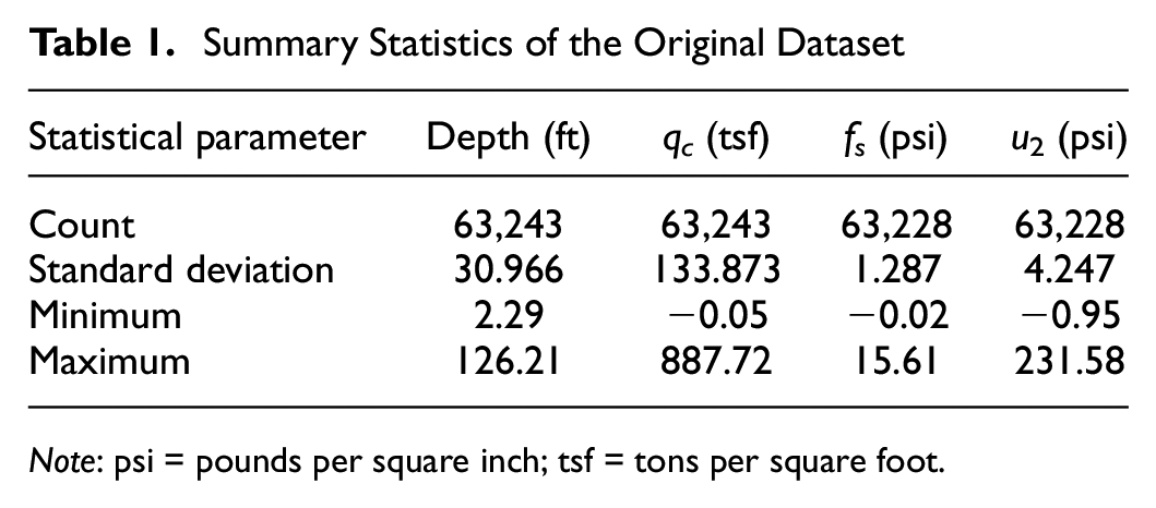
Python was used to preprocess and integrate the CPT data and soil classification results for ML analysis. CPT data and soil classification data were captured from the adjacent CPT soundings and boreholes. The Python script automated the extraction of specific columns from the exported CPT data files and incorporated corresponding soil classifications based on depth conditions. In addition, a comprehensive dataset was generated by merging all the individual data files, while eliminating rows with missing Unified Soil Classification System (USCS) Group Name values. This was necessary as some of the boreholes in the vicinity of CPT soundings were drilled to shallow depths for the purpose of a soil survey and therefore did not have the same depth as the CPT soundings near them. A selection was made from the available CPT soundings and boreholes with soil classification data, consisting of a total of 90 groups of coupled CPT soundings and boreholes (180 total test locations) within a distance of 50 ft or less from each other. The depths of the boreholes ranged from 2.29 to 126.21 ft. After cleaning the data and removing records with missing data, we ended up with 63,243 records of raw CPT data and soil classifications. The resulting dataset was used for subsequent ML modeling and analysis. Table 1 shows the statistics of the CPT data. The number of data counts for q_c, f_s, and u₂ are not the same because different CPT soundings and soil types may have varying availability of data points or measurements at different depths, leading to discrepancies in the counts across these parameters.

Table 1.

Summary Statistics of the Original Dataset

Statistical parameter	Depth (ft)	q_c (tsf)	f_s (psi)	u₂ (psi)
Count	63,243	63,243	63,228	63,228
Standard deviation	30.966	133.873	1.287	4.247
Minimum	2.29	−0.05	−0.02	−0.95
Maximum	126.21	887.72	15.61	231.58

Note: psi = pounds per square inch; tsf = tons per square foot.

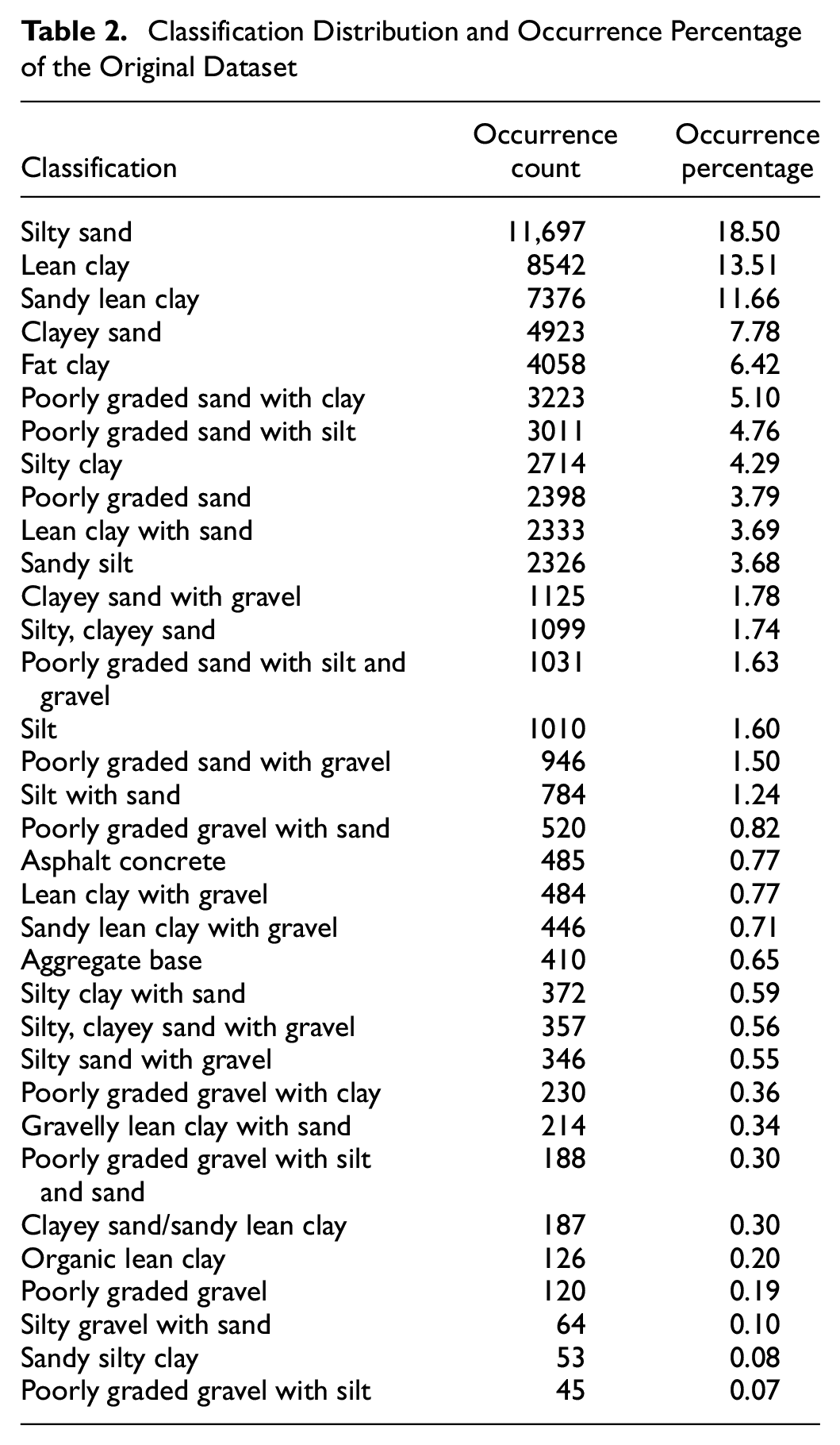
Overall, there was a total of 34 different USCS classifications in the records. Table 2 shows the variation of the classifications together with their occurrence counts and occurrence percentages for each record.

Table 2.

Classification Distribution and Occurrence Percentage of the Original Dataset

Classification	Occurrence count	Occurrence percentage
Silty sand	11,697	18.50
Lean clay	8542	13.51
Sandy lean clay	7376	11.66
Clayey sand	4923	7.78
Fat clay	4058	6.42
Poorly graded sand with clay	3223	5.10
Poorly graded sand with silt	3011	4.76
Silty clay	2714	4.29
Poorly graded sand	2398	3.79
Lean clay with sand	2333	3.69
Sandy silt	2326	3.68
Clayey sand with gravel	1125	1.78
Silty, clayey sand	1099	1.74
Poorly graded sand with silt and gravel	1031	1.63
Silt	1010	1.60
Poorly graded sand with gravel	946	1.50
Silt with sand	784	1.24
Poorly graded gravel with sand	520	0.82
Asphalt concrete	485	0.77
Lean clay with gravel	484	0.77
Sandy lean clay with gravel	446	0.71
Aggregate base	410	0.65
Silty clay with sand	372	0.59
Silty, clayey sand with gravel	357	0.56
Silty sand with gravel	346	0.55
Poorly graded gravel with clay	230	0.36
Gravelly lean clay with sand	214	0.34
Poorly graded gravel with silt and sand	188	0.30
Clayey sand/sandy lean clay	187	0.30
Organic lean clay	126	0.20
Poorly graded gravel	120	0.19
Silty gravel with sand	64	0.10
Sandy silty clay	53	0.08
Poorly graded gravel with silt	45	0.07

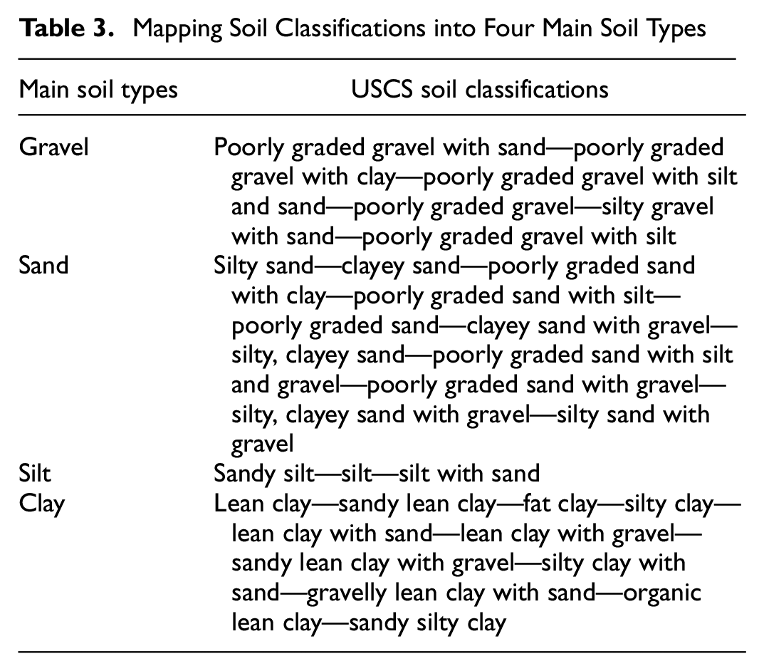
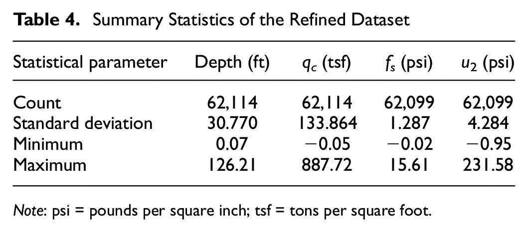
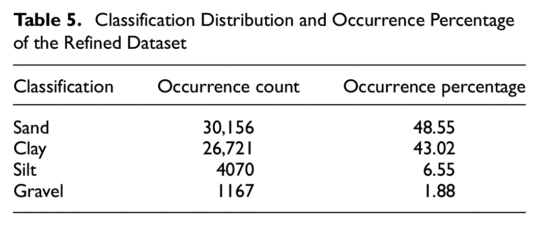
In the next process, we refined the data to only include the records that belonged to the categories of “Sand,” “Silt,” “Clay,” or “Gravel” in the USCS Group Name. This filtering step aimed to exclude any records with USCS Group Name values outside of these specified categories. As a result, we obtained a new dataset that contained a refined subset of data focused exclusively on the desired categories. To do this, we mapped certain values to their corresponding group, as shown in Table 3. This mapping ensured that only records falling into these designated soil types were included in the resulting dataset. The refined dataset was used for similar ML analyses as the original dataset. Table 4 shows the summary statistics of the refined dataset and Table 5 shows the classification distribution and occurrence percentage of the refined dataset.

Table 3.

Mapping Soil Classifications into Four Main Soil Types

Main soil types	USCS soil classifications
Gravel	Poorly graded gravel with sand—poorly graded gravel with clay—poorly graded gravel with silt and sand—poorly graded gravel—silty gravel with sand—poorly graded gravel with silt
Sand	Silty sand—clayey sand—poorly graded sand with clay—poorly graded sand with silt—poorly graded sand—clayey sand with gravel—silty, clayey sand—poorly graded sand with silt and gravel—poorly graded sand with gravel—silty, clayey sand with gravel—silty sand with gravel
Silt	Sandy silt—silt—silt with sand
Clay	Lean clay—sandy lean clay—fat clay—silty clay—lean clay with sand—lean clay with gravel—sandy lean clay with gravel—silty clay with sand—gravelly lean clay with sand—organic lean clay—sandy silty clay

Table 4.

Summary Statistics of the Refined Dataset

Statistical parameter	Depth (ft)	q_c (tsf)	f_s (psi)	u₂ (psi)
Count	62,114	62,114	62,099	62,099
Standard deviation	30.770	133.864	1.287	4.284
Minimum	0.07	−0.05	−0.02	−0.95
Maximum	126.21	887.72	15.61	231.58

Note: psi = pounds per square inch; tsf = tons per square foot.

Table 5.

Classification Distribution and Occurrence Percentage of the Refined Dataset

Classification	Occurrence count	Occurrence percentage
Sand	30,156	48.55
Clay	26,721	43.02
Silt	4070	6.55
Gravel	1167	1.88

Machine Learning Algorithms

ML is a branch of computer science that focuses on extracting valuable insights from data. ML algorithms and techniques are employed to automatically enhance performance by simulating human learning processes. These techniques have been previously used in different areas of geotechnical engineering (17, 18). The core concept of ML involves constructing a model that learns from a designated dataset, commonly referred to as a “training dataset,” through a process known as learning or training. Once the model has undergone the learning phase, it becomes capable of making predictions or decisions. This learning process, which involves mapping input features to corresponding targets, is known as supervised learning.

In the current study analysis, ML algorithms are utilized to predict soil classifications based on raw CPT data, including depth, q_c, f_s, and u₂. The dataset was split into a training set and a test set, with 80% of the samples used for training and 20% for testing. For our analysis, we applied five commonly used ML algorithms: extreme gradient boosting (XGBoost), logistic regression, the support vector machine (SVM), the random forest (RF), and K-nearest neighbors (KNN). These algorithms are all classification models that are used to predict a categorical target variable based on a set of input variables. Overall, the performance of each algorithm is highly dependent on the specific dataset and the tuning of their parameters. Therefore, it is important to evaluate multiple models and their parameters to find the best-performing model for the given problem.

Logistic Regression

Logistic regression is a statistical method employed in binary classification tasks, serving as a fundamental tool for predictive modeling. It models the probability of an event occurrence through the logistic function, transforming a linear combination of input features into probabilities within the range of 0–1. The logistic regression equation encapsulates the relationship between the input variables and the binary outcome, with coefficients determined through the process of maximum likelihood estimation. This method is particularly advantageous for scenarios where the dependent variable represents a categorical outcome with two possible states, such as success or failure, presence or absence, making it applicable in various academic domains and research disciplines. Logistic regression has been previously used for evaluating soil liquefaction probability using CPT data ( 19 ).

In our model, we used the default settings for logistic regression, which include the “l2” penalty and an inverse of regularization strength of 1.0.

Support Vector Machine

The SVM is a nonlinear model that works well with both linearly separable and nonlinearly separable datasets. It tries to find a hyperplane that separates the classes with the maximum margin between them, for example, assuming a scenario with two distinct sets or classes of data points. The objective is to create a hyperplane that maximizes the distance between the nearest point from each class and the hyperplane. The data points that are closest to the hyperplane, or from which the distance to the hyperplane is calculated, are referred to as support vectors. Figure 3 visualizes the hyperplane and support vectors in the context of a binary classification problem. The SVM has been successfully applied by researchers in various geotechnical engineering domains, such as soil classification, bearing capacity, and soil compressibility. In these applications, the SVM has demonstrated excellent predictive performance (12, 20 –22).

Figure 3.

Support vector machine for binary classification.

In our model, we used the default settings for the SVM, which include the radial basis function (RBF) kernel, regularization parameter C = 1.0, and default gamma setting.

Random Forest

The RF is a versatile ensemble learning method widely used across various domains for predictive modeling. It goes beyond the capabilities of individual decision trees by harnessing the strength of multiple trees to create a more accurate and resilient model. One of its distinctive features is the random selection of input variables for each decision tree, introducing diversity into the ensemble and mitigating overfitting risks, thereby enhancing the model’s ability to generalize.

In our analysis, we utilized 100 decision tree estimators within the RF framework. Each decision tree is built using a subset of input variables chosen at random, fostering diversity among the trees. The “Gini” criterion was employed for splitting nodes in these decision trees. The Gini index, a measure of impurity or disorder, guides the selection of optimal splits during the tree-building process. By minimizing the Gini index at each node, the algorithm effectively partitions the input space. The ensemble then aggregates predictions from all individual trees, yielding a more robust and accurate final prediction. This utilization of randomness and aggregation principles enhances the overall performance of the RF method in predictive modeling tasks. The RF has demonstrated its efficacy in predicting a wide range of geotechnical parameters and phenomena. It has been successfully utilized in soil classification, estimation of undrained shear strength, assessment of settlement induced by seismic forces, prediction of settlement in shallow foundations, evaluation of pile drivability, and determination of liquefaction potential based on CPT and shear wave velocity data, among other applications ( 23 – 28 ).

K-Nearest Neighbors

KNN is a non-parametric classification algorithm that ascertains the class of a new data point by locating its KNN in the feature space, utilizing a distance metric such as Euclidean distance. Subsequently, the algorithm assigns the new point a class determined by the majority class among its K neighbors, rendering it an intuitive and straightforward approach. The selection of K assumes significance, striking a balance between sensitivity to noise for smaller K values and the smoothing of decision boundaries for larger K values. While KNN excels at capturing nonlinear patterns, its sensitivity to feature scale and quality, along with potential susceptibility to the curse of dimensionality in high-dimensional spaces, warrants careful consideration. Operating on the principle of proximity, KNN identifies the K-closest neighbors to a test sample and classifies it based on the predominant label among those neighbors, with the choice of K playing a pivotal role in influencing the model’s performance and computational efficiency ( 29 ).

Researchers have successfully applied KNN to various geotechnical engineering problems, including landslide susceptibility assessment, soil classification, slope stability analysis, and rock deformation prediction, because of its simplicity and promising results ( 30 – 34 ). In our analysis, we used the default settings for KNN, including K = 5 and the Minkowski distance metric.

Extreme Gradient Boosting

XGBoost is a powerful ML library renowned for its effectiveness in both regression and classification tasks. It operates as an ensemble learning method that combines the predictions of multiple weak decision trees, offering superior predictive performance. Notable for its efficiency, scalability, and regularization techniques, XGBoost has become a staple in various domains, including scientific research and analysis.

Within the XGBoost library, the extreme gradient boosting classifier (XGBClassifier) stands out as a dedicated implementation tailored specifically for classification tasks. Leveraging the principles of XGBoost, the XGBClassifier optimizes a specified loss function by iteratively adding decision trees, guided by the gradients of the loss. This implementation incorporates features such as early stopping, proficient handling of missing values, and the ability to interpret feature importance, making it a robust and versatile tool for accurate classification in diverse applications. The subsequent sections delve into the intricacies of XGBoost and the specialized features that distinguish the XGBClassifier in the context of classification tasks.

Because of its fast computation and impressive performance on complex datasets, the XGBoost algorithm has gained significant popularity among researchers working on geotechnical problems. It has proven particularly useful in predicting essential parameters such as pile-bearing capacity, slope stability, undrained shear strength, and subsurface geology. The ability of XGBoost to handle intricate data and deliver accurate predictions has made it a preferred choice for geotechnical analysis (28, 35–37).

Performance Evaluation Metrics

We evaluated the performance of ML methods by using several metrics, including accuracy, precision, recall, and F1-score.

Accuracy is a performance metric used to evaluate the effectiveness of a classification model. It measures the proportion of correct predictions that the model made out of all the predictions it made. In other words, it calculates the ratio of the number of correct predictions to the total number of predictions. It is a simple and easy-to-understand metric that provides an overall measure of the model’s performance. However, accuracy can be misleading when the classes in the data are imbalanced. For instance, if the majority of the data belongs to one class, a model that always predicts that class will have high accuracy, which may not necessarily be a good model.

Precision, an essential metric for assessing classification models, quantifies the proportion of true positive predictions among all positive predictions generated by the model. In simpler terms, it computes the ratio of true positive predictions to the total number of positive predictions. Precision assumes particular significance when the consequences of a false positive prediction are substantial. This is particularly evident in domains such as medical diagnosis, where a false positive prediction can entail significant costs because of the potential initiation of unnecessary treatment. In essence, a “true positive” denotes the model’s accurate prediction of the positive class, while a “false positive” signifies an instance in which the model erroneously anticipates the positive class.

Recall is a metric that measures the proportion of true positive predictions out of all actual positive cases in the data. In other words, it calculates the ratio of the number of true positive predictions to the total number of positive cases in the data. Recall is useful when the cost of a false negative prediction is high. For example, in fraud detection, the cost of a false negative prediction can be high, as it may lead to financial losses.

The F1-score is the harmonic mean of precision and recall. It is a single metric that takes both precision and recall into account. The F1-score is a useful metric when there is an imbalance between the classes in the data. It is also useful when both precision and recall are equally important, and there is a need to balance the trade-off between them. In addition to its utility in addressing class imbalances and balancing the trade-off between precision and recall, the F1-score is particularly beneficial in situations where the cost of false positives and false negatives is not significantly different. This metric provides a consolidated measure that considers both false positives (precision) and false negatives (recall), making it effective for evaluating the overall performance of a classification model, especially in scenarios where achieving a balance between precision and recall is critical for decision-making.

Results

The results of our analysis demonstrated that the RF algorithm outperformed other ML methods in predicting soil classification based on CPT data for both original and refined datasets. Table 6 presents the accuracy, F1-score, precision, and recall results of the various ML methods for the original dataset. The RF method achieved the best results with an accuracy of 83.6%, F1-score of 0.836, precision of 0.838, and recall of 0.836. This indicates a high level of reliability in classifying soil samples using the selected features of depth, q_c, f_s, and u₂. On the other hand, logistic regression had the least reliable result with an accuracy of 51.0%, F1-score of 0.505, precision of 0.521, and recall of 0.596.

Table 6.

Performance of the Various Machine Learning Methods for the Original Dataset

Model	Accuracy (%)	F1-score	Precision	Recall
RF	83.6	0.836	0.838	0.836
KNN	69.6	0.695	0.699	0.696
SVM	51.2	0.594	0.573	0.598
Logistic regression	51.0	0.505	0.521	0.596
XGBoost	71.8	0.718	0.724	0.718

Note: RF = random forest; KNN = K-nearest neighbors; SVM = support vector machine; XGBoost = extreme gradient boosting.

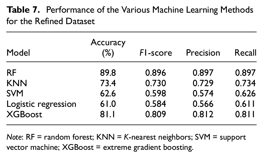
Table 7 compares the performance of different ML algorithms on refined datasets. The RF consistently showed the best results with an F1-score of 0.896. The XGBoost and KNN classifiers also performed well, achieving F1-scores of 0.809 and 0.730, respectively. The SVM and logistic regression exhibited F1-scores of 0.598 and 0.584, respectively. These findings emphasize the potential of ML algorithms, particularly the RF algorithm, in accurately predicting soil classification using CPT data.

Table 7.

Performance of the Various Machine Learning Methods for the Refined Dataset

Model	Accuracy (%)	F1-score	Precision	Recall
RF	89.8	0.896	0.897	0.897
KNN	73.4	0.730	0.729	0.734
SVM	62.6	0.598	0.574	0.626
Logistic regression	61.0	0.584	0.566	0.611
XGBoost	81.1	0.809	0.812	0.811

Note: RF = random forest; KNN = K-nearest neighbors; SVM = support vector machine; XGBoost = extreme gradient boosting.

Eventually, we analyzed the CPT parameter importance in predicting soil types using the RF classifier. The dataset used in the analysis consisted of CPT parameters (depth, q_c, f_s, and u₂) and the corresponding soil classification labels. Missing values in the dataset are handled using simple imputation. The RF classifier is then trained on the dataset to determine the importance of each CPT parameter in predicting soil types. The importance scores are computed as shown in the pie chart in Figure 4, which provides insights into the significance of CPT parameters in soil classification. Depth had the highest importance among the rest of the CPT data, with a 37.4% importance value, followed by q_c with 23.7%, u₂ with 21.6%, and f_s with 17.3%.

Figure 4.

Importance of cone penetration test parameters in soil type prediction.

Conclusion

This study explores the potential of ML techniques to automate and enhance soil classification based on CPT data. The results demonstrate that ML algorithms, particularly the RF algorithm, outperform other methods in predicting soil classification. The RF model exhibits superior performance, achieving an F1-score of 0.896 when applied to the refined dataset. Feature importance analysis reveals that the depth parameter holds the highest importance, followed by cone tip resistance (q_c), pore pressure reading (u₂), and sleeve friction (f_s), emphasizing their significant influence in determining soil classification based on CPT data. These findings suggest that ML algorithms can significantly improve the interpretation of CPT data, enhancing soil classification reliability and offering potential benefits to the field of geotechnical engineering. This study contributes to the growing body of research on the application of ML in geotechnical engineering, highlighting the promise of data-driven approaches to improve soil classification accuracy and efficiency. The importance of this research lies in its potential to transform current soil classification practices, making them more accurate, efficient, and informed by leveraging advanced ML techniques.

Limitations

While this study has made significant strides in leveraging ML techniques for soil classification based on CPT data, it is essential to acknowledge certain limitations. One notable limitation is the dependency on the quality and quantity of the available CPT data. The effectiveness of ML algorithms, particularly the RF model, is contingent on the diversity and representativeness of the training dataset. In instances where data may be limited or biased toward certain soil types or conditions, the model’s performance could be affected. In addition, the generalizability of the findings may be influenced by the specific characteristics of the studied site, and caution should be exercised when applying the results to different geological contexts. Another limitation pertains to the reliance on selected features, such as depth, cone tip resistance (q_c), pore pressure reading (u₂), and sleeve friction (f_s). While these features demonstrated high importance in the analysis, there may be other relevant parameters not considered in this study. Furthermore, the study focused primarily on the prediction accuracy of soil classification and did not delve into the uncertainties associated with individual predictions. Addressing these limitations in future research could involve enhancing dataset diversity, exploring additional influential features, considering site-specific factors, and incorporating uncertainty analyses to provide a more comprehensive evaluation of the ML models’ performance.

Footnotes

Author Contributions

The authors confirm contribution to the paper as follows: study conception and design: M. Fatehnia; data collection: S. Amiri; analysis and interpretation of results: M. Fatehnia, V. Mahmoudabadi; draft manuscript preparation: M. Fatehnia, V. Mahmoudabadi, S. Amiri. All authors reviewed the results and approved the final version of the manuscript.

Declaration of Conflicting Interests

The author(s) declared no potential conflicts of interest with respect to the research, authorship, and/or publication of this article.

Funding

The author(s) received no financial support for the research, authorship, and/or publication of this article.

ORCID iDs

Milad Fatehnia

Sharid Amiri

References

Fatehnia

Deaton

A Geotechnical Data Archive Isn’t Geotechnical Data. GeoStrata Magazine Archive, Vol. 27, No. 5, 2023, pp. 42–49.

Fatehnia

Deaton

Geotechnical Data Analytics and Data Mining Using Microsoft Power BI. Proc. Geo-Congress, ASCE, Charlotte, NC, 2022, pp. 553–560.

Robertson

P. K.

Soil Behaviour Type from the CPT: An Update. Proc., 2nd International Symposium on Cone Penetration Testing, Huntington Beach, CA, 2010.

Garcia

Ovando-Shelley

Gutierrez

Garcia

Liquefaction Assessment Through Machine Learning. Proc., 15th World Conference on Earthquake Engineering, Lisboa, Portugal, 2012.

Cho

S. E.

Probabilistic Stability Analyses of Slopes Using the ANN-Based Response Surface. Computers and Geotechnics, Vol. 36, No. 5, 2009, pp. 787–797.

Peng

X. Y.

D. Q.

Jiang

S. H.

Zhang

L. M.

Slope Safety Evaluation by Integrating Multi-Source Monitoring Information. Structural Safety, Vol. 49, 2014, pp. 65–74.

Bhargavi

Jyothi

D. S.

Soil Classification Using Data Mining Techniques: A Comparative Study. International Journal of Engineering Trends and Technology, Vol. 2, No. 1, 2011, pp. 55–59.

Demir

Sahin

E. K.

Comparison of Tree-Based Machine Learning Algorithms for Predicting Liquefaction Potential Using Canonical Correlation Forest, Rotation Forest, and Random Forest Based on CPT Data. Soil Dynamics and Earthquake Engineering, Vol. 154, 2022, p. 107130, https://doi.org/10.1016/j.soildyn.2021.107130.

Ghaderi

Abbaszadeh Shahri

Larsson

An Artificial Neural Network-Based Model to Predict Spatial Soil Type Distribution Using Piezocone Penetration Test Data (CPTu). Bulletin of Engineering Geology and the Environment, Vol. 78, No. 6, 2019, pp. 4579–4588.

10.

Kohestani

V. R.

Hassanlourad

Ardakani

Evaluation of Liquefaction Potential Based on CPT Data Using Random Forest. Natural Hazards, Vol. 79, No. 2, 2015, pp. 1079–1089.

11.

Kurup

P. U.

Griffin

E. P.

Prediction of Soil Composition from CPT Data Using General Regression Neural Network. Journal of Computing in Civil Engineering, Vol. 20, No. 4, 2006, pp. 281–289.

12.

Rauter

Tschuchnigg

CPT Data Interpretation Employing Different Machine Learning Techniques. Geosciences, Vol. 11, No. 7, 2011, p. 265.

13.

Tsiaousi

Travasarou

Drosos

Ugalde

Chacko

Machine Learning Applications for Site Characterization Based on CPT Data. Proc., Geotechnical Earthquake Engineering and Soil Dynamics V: Slope Stability and Landslides; Laboratory Testing and In Situ Testing, American Society of Civil Engineers, Reston, VA, 2018, pp. 461–472.

14.

Zhang

J. Z.

Zhang

D. M.

Huang

H. W.

Phoon

K. K.

Tang

Hybrid Machine Learning Model with Random Field and Limited CPT Data to Quantify Horizontal Scale of Fluctuation of Soil Spatial Variability. Acta Geotechnica, Vol. 17, No. 4, 2022, pp. 1129–1145.

15.

Zhao

Duan

Cai

A Novel PSO-KELM Based Soil Liquefaction Potential Evaluation System Using CPT and Vs Measurements. Soil Dynamics and Earthquake Engineering, Vol. 150, 2021, p. 106930.

16.

Mayne

Saftner

Dagger

Dasenbrock

Cone Penetration Testing Manual for Highway Geotechnical Engineers. Georgia Institute of Technology, Atlanta, Georgia, 2018.

17.

Fatehnia

Automated Method for Determining Infiltration Rate in Soils. Electronic thesis, treatises and dissertations. Paper 9327, Florida State University, Tallahassee, Florida, 2015.

18.

Fatehnia

Amirinia

A Review of Genetic Programming and Artificial Neural Network Applications in Pile Foundations. International Journal of Geo-Engineering, Vol. 9, No. 2, 2018, pp. 1–20.

19.

Lai

S. Y.

Chang

W. J.

Lin

P. S.

Logistic Regression Model for Evaluating Soil Liquefaction Probability Using CPT Data. Journal of Geotechnical and Geoenvironmental Engineering, Vol. 132, No. 6, 2006, pp. 694–704.

20.

Alkroosh

I. S.

Bahadori

Nikraz

Bahadori

Regressive Approach for Predicting Bearingcapacity of Bored Piles from Cone Penetration Test Data. Journal of Rock Mechanics and Geotechnical Engineering, Vol. 7, No. 5, 2015, pp. 584–592.

21.

Kirts

Panagopoulos

O. P.

Xanthopoulos

Nam

B. H.

Soil-Compressibility Prediction Models Using Machine Learning. Journal of Computing in Civil Engineering, Vol. 32, No. 1, 2018, p. 04017067.

22.

Kordjazi

Nejad

F. P.

Jaksa

M. B.

Prediction of Ultimate Axial Load-Carrying Capacity of Piles Using a Support Vector Machine Based on CPT Data. Computers and Geotechnics, Vol. 55, 2014, pp. 91–102.

23.

Liu

Macedo

Machine Learning-Based Models for Estimating Seismically-Induced Slope Displacements in Subduction Earthquake Zones. Soil Dynamics and Earthquake Engineering, Vol. 160, 2022, p. 107323. https://doi.org/10.1016/j.soildyn.2022.10732.

24.

Macedo

Liu

Soleimani

Machine-Learning-Based Predictive Models for Estimating Seismically-Induced Slope Displacements. Soil Dynamics and Earthquake Engineering, Vol. 148, 2021, p. 106795. https://doi.org/10.1016/j.soildyn.2021.106795.

25.

Shoarinejad

Güler

Özturan

Evaluation of Liquefaction Potential Using Random Forest Method and Shear Wave Velocity Results. Proc., International Conference on Applied Mathematics & Computational Science (ICAMCS.NET), Budapest, Hungary, IEEE, New York, 2018, pp. 23–26.

26.

Pham

T. A.

Tran

V. Q.

Developing Random Forest Hybridization Models for Estimating the Axial Bearing Capacity of Pile. Plos One, Vol. 17, No. 3, 2022, p. 0265747.

27.

Zhang

Wang

Samui

Assessment of Pile Drivability Using Random Forest Regression and Multivariate Adaptive Regression Splines. Georisk: Assessment and Management of Risk for Engineered Systems and Geohazards, Vol. 15, No. 1, 2021, pp. 27–40.

28.

Zhang

Zhong

Wang

Prediction of Undrained Shear Strength Using Extreme Gradient Boosting and Random Forest Based on Bayesian Optimization. Geoscience Frontiers, Vol. 12, No. 1, 2021, pp. 469–477.

29.

Peterson

L. E.

K-Nearest Neighbor. Scholarpedia, Vol. 4, No. 2, 2009, p. 1883.

30.

Carvalho

L. O.

Ribeiro

D. B.

Soil Classification System from Cone Penetration Test Data Applying Distance-Based Machine Learning Algorithms. Soils and Rocks, Vol. 42, No. 2, 2019, pp. 167–178.

31.

Koopialipoor

Asteris

P. G.

Mohammed

A. S.

Alexakis

D. E.

Mamou

Armaghani

D. J.

Introducing Stacking Machine Learning Approaches for the Prediction of Rock Deformation. Transportation Geotechnics, Vol. 34, 2022, p. 100756. https://doi.org/10.1016/j.trgeo.2022.100756.

32.

Marjanovic

Bajat

Kovacevic

Landslide Susceptibility Assessment with Machine Learning Algorithms. Proc., International Conference on Intelligent Networking and Collaborative Systems, IEEE Computer Society, Washington, D.C., 2009, pp. 273–278.

33.

Paraskevas

Constantinos

Dimitrios

Ioanna

Landslide Susceptibility Assessments Using the K-Nearest Neighbor Algorithm and Expert Knowledge. Case Study of the Basin of Selinounda River, Achaia County, Chania, Crete, Greece, 2015, pp. 10–14.

34.

Seman

Shoop

McGrath

S. P.

Rolling

R. S.

Soil Strength Prediction with K-Nearest Neighbor Method. Proc., 59th Canadian Geotechnical Conference, Vancouver, BC, Canada, 2006.

35.

Amjad

Ahmad

Wróblewski

Kamiński

Amjad

Prediction of Pile Bearing Capacity Using Xgboost Algorithm: Modeling and Performance Evaluation. Applied Sciences, Vol. 12, No. 4, 2022, p. 2126.

36.

Bharti

J. P.

Mishra

Sathishkumar

V. E.

Cho

Samui

Slope Stability Analysis Using RF, GBM, CART, BT, and XGBoost. Geotechnical and Geological Engineering, Vol. 39, No. 5, 2011, pp. 3741–3752.

37.

Shi

Wang

Development of Subsurface Geological Cross-Section from Limited Site-Specific Boreholes and Prior Geological Knowledge Using Iterative Convolution XGBoost. Journal of Geotechnical and Geoenvironmental Engineering, Vol. 147, No. 9, 2021, p. 04021082.