Training Vehicle Detection and Classification Models with Less Data: An Active Learning Approach

Abstract

The application of computer vision in transportation engineering has facilitated real-time traffic flow optimization, vehicle counting, anomaly detection, and ameliorated transportation safety. Most vision systems are, however, developed through a supervised learning process, which can be data hungry and costly because it requires manual annotation of objects from a variety of sources. The general rule of thumb for building accurate and transferrable vision models has been to increase the quality, diversity, and quantity of the annotated datasets used in model training. This paper presents a simple, yet efficient active learning framework that significantly reduces the number of annotations needed to build a state-of-the-art vehicle detection and classification model. To achieve this, we first leverage a vision transformer that generates embeddings rich with information needed to quantify the similarity and diversity between images in a two-dimensional embedding space. To select which images from the embedding space should be annotated, we propose a scoring and sampling strategy that minimizes class imbalance and model uncertainty through an iterative process. The latest iteration of the You Only Look Once (YOLO) model, YOLOv8, is used as the active learner. We compare the efficacy of our proposed active learning methods with models developed at much higher sampling rates using the mean average precision. The models developed were also integrated with tracking algorithms to evaluate differences in accuracy for vehicle counts and their practical implications for direction counts.

Keywords

data and data science artificial intelligence deep learning machine learning (artificial intelligence)machine vision supervised learning

The advancement of artificial intelligence has significantly influenced the transportation engineering domain, particularly owing to the substantial contribution of deep learning. Deep learning models have played a crucial role in automating vehicle detection and counting, pavement monitoring, and traffic anomaly detection. However, deep learning models have certain drawbacks, and one well-known limitation is their need for extensive amounts of data to ensure model generalizability. Data labeling using human annotators can be time-consuming and expensive. The overarching goal of this study is to develop an active learning (AL) model that significantly reduces the amount of labeled data needed to build a robust vision system.

Alternative learning strategies have been explored to alleviate the aforementioned challenges. For example, transfer learning ( 1 ) uses pre-trained weights from a larger dataset and fine-tunes the weights on a smaller target dataset to achieve state-of-the-art results. Even though this method has achieved significant results in the past, recent findings have shown that it faces the limitation of overfitting and domain shift adaptation when there is a significant discrepancy in the data distribution of the target dataset and pre-trained data ( 2 , 3 ). Few-shot learning ( 4 ), on the other hand, equips a pre-trained model with the ability to recognize new classes using only a few labeled samples per class, achieved through meta-learning techniques, enabling it to adapt quickly to new tasks with limited data. Contrastingly, few-shot learning may struggle with highly complex or fine-grained classes that require a more extensive set of examples to capture all the nuances and variations within the class ( 5 , 6 ). In zero-shot learning ( 7 ), a model is pre-trained on known classes (seen classes) and later applied to classify unknown classes (unseen classes) without further training, leveraging auxiliary information such as semantic representations (e.g., class attributes or descriptions) to match the unseen class attributes with the closest known classes and make predictions based on the best match. Zero-shot learning faces challenges related to bias, domain shift, hubness, and semantic loss. The model may be biased toward predicting unseen samples as belonging to seen classes, struggle with domain shifts between training and testing data, encounter hubness problems in high-dimensional spaces, and lose important latent information that is relevant for distinguishing unseen classes ( 8 , 9 ). AL enables the model to actively select the most informative examples for labeling, ensuring an efficient use of annotation resources and allowing for improved model performance with fewer labeled examples. AL directly addresses data scarcity, making it the preferred choice for data-efficient learning and practical real-world applications where labeled data acquisition is costly or time-consuming.

AL is a learning paradigm that reduces reliance on human annotators by allowing the model to elect informative training samples for annotation rather than training the model on the entire training set while producing comparable, if not better, model performance. There are three AL strategies, namely membership query synthesis ( 10 ), stream-based selective sampling ( 11 ), and the pool-based approach ( 12 ). In membership query synthesis, the AL algorithm can request an oracle to label a sample from an unlabeled pool or an artificial sample that the learner generates independently. Stream-based selective sampling is associated with online real-time sampling from a stream of unlabeled data to annotate and incrementally adjust the labeled dataset. In a pool-based method, the active learner samples from a fixed pool containing an evenly distributed subset of unlabeled data ( 13 ). While AL is a valuable approach, it has some limitations. One notable limitation is the possibility of sampling bias, which occurs when the selection strategy fails to consider the dataset’s distribution, resulting in a biased model that focuses on specific regions of the data space. Also, the effectiveness of AL is dependent on accurate uncertainty estimation to select informative samples, which can be difficult for some models or complex data distributions. Another noteworthy limitation occurs with high-dimensional data, where the increasing number of samples required to represent the data space accurately can reduce the effectiveness of AL ( 14 , 15 ).

The main goal of this study is to significantly reduce the number of annotations required to train a state-of-the-art object recognition model without sacrificing accuracy. To achieve this, we learn a single embedding space that explains the diversity within a large database of images and uniquely clusters them based on their unique characteristics. An iterative sampling strategy is subsequently used to score and select the most informative images that should be annotated to train a high-performance model. Our entire framework is illustrated in Figure 1. We show that the resulting embedding space and the sampling strategy adopted results in a model with comparable performance and, in some cases, higher than those trained on much larger datasets. With respect to the ability to generalize to new, previously unseen data, the developed framework still showed promise against default large data-driven models. Ultimately, we integrated the developed AL models with state-of-the-art tracking algorithms for directional traffic counts and observed insignificant differences in count accuracy when compared with models trained with larger datasets. This research contributes significantly to four key aspects.

We construct an embedding space that effectively represents the diversity of a large image database, enabling efficient clustering of images based on their inherent characteristics.

We develop a novel iterative sampling strategy to score and select the most informative images for annotation, leading to improved model efficiency with reduced labeled samples.

We pioneer the application of AL for object recognition, tracking, and counting in the domain of transportation engineering, providing valuable insights into its potential for real-world applications with reduced annotation efforts.

We conduct a comparative analysis between the developed AL model and a baseline fully trained model, evaluating vehicle recognition, tracking, and counting performance and assessing generalizability to validate the AL framework's efficiency.

The rest of this paper is organized as follows. In the second section, we review the existing literature on AL. We describe our proposed AL methodology and the options available for each cycle phase in the third section. The fourth section explains the experimental setup and discusses the study’s findings. Finally, the fifth section concludes the study and suggests some future research.

Figure 1.

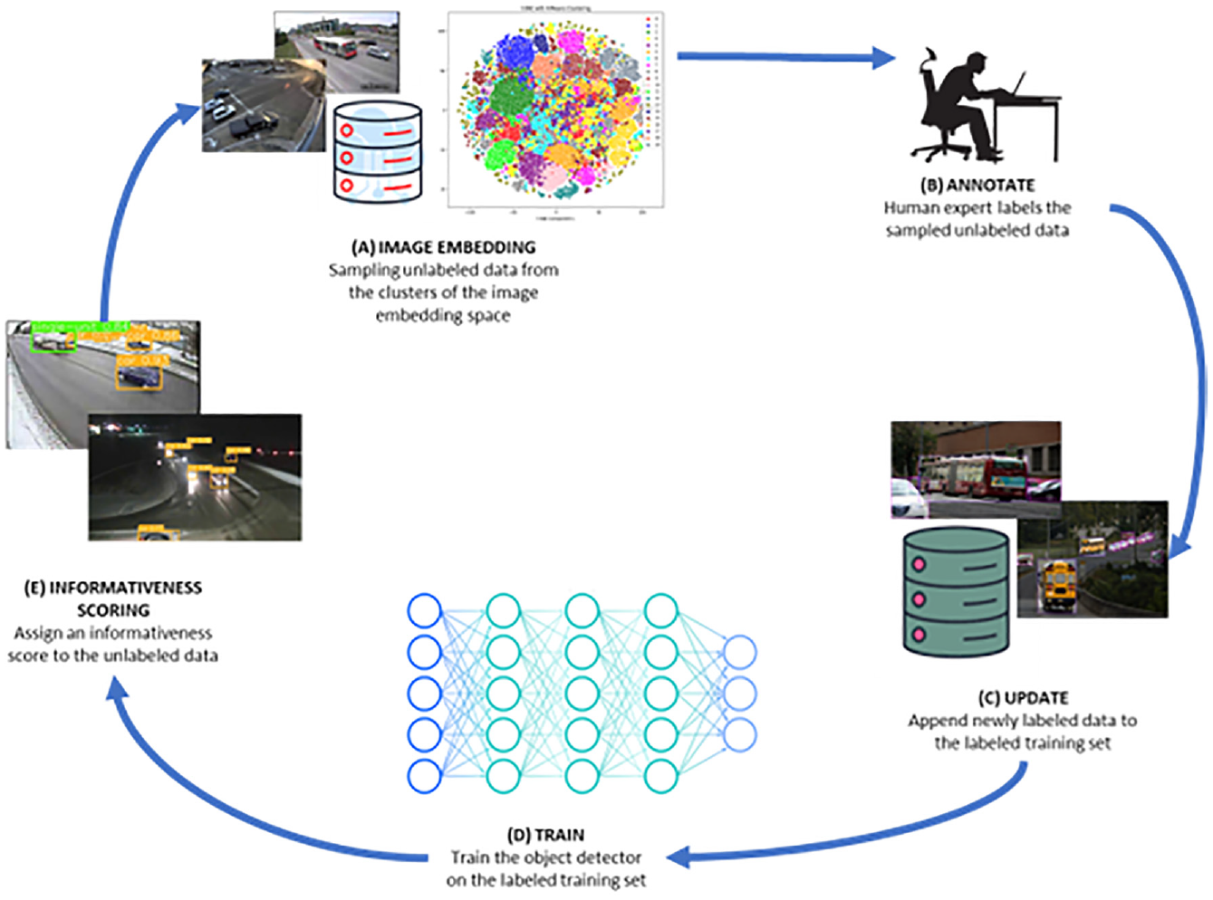
Proposed active learning cycle.

Literature Review

Deep learning-based algorithms play a pivotal role in vehicle detection for intelligent transportation systems, addressing challenges posed by diverse environmental conditions and the real-time processing demands of computer vision. Khalifa et al. ( 16 ) employed a You Only Look Once (YOLO; YOLOv4) model with optimized bounding box prediction using the k-means algorithm on a bidirectional highway dataset, categorizing vehicles into four classes: car, van, bus, and others. To mitigate the labor-intensive process of manual annotations, data augmentation techniques were utilized. While outperforming the original YOLOv5 model, this approach faced challenges in low-light conditions because of diminished visibility of distinctive features for various vehicle classes. Similarly, Farid et al. ( 17 ) utilized a pre-trained YOLO-v5 on the PKU, COCO, and DAWN datasets, featuring classes such as car, motorcycle, trucks, and person. Using a public dataset and applying data augmentation, the model excelled but struggled with occluded vehicles, prompting a recommendation for future work on moving vehicles with tracking capabilities. In contrast, Zhang et al. ( 18 ) proposed an enhanced YOLO v5 model, covering eight classes, namely bus, minibus, family sedan, taxi, heavy truck, truck, SUV, and special vehicles with a semi-automatic annotation approach to reduce manual effort. Although the model performed well, the authors suggested incorporating more diverse scenes for training to enhance generalizability. Nguyen ( 19 ) followed a similar path, employing a modified YOLOv3 for a drone-based system with classes grouped under “vehicle,” addressing data imbalance and emphasizing robustness in adverse weather. The model demonstrated improved accuracy and faster inference for practical traffic monitoring, yet faced limitations in adverse weather, low-light conditions, and highly congested traffic scenes with overlapping vehicles. Yan et al. ( 20 ) contributes a significant dataset with 13 vehicle classes, including cars, vans, dump trucks, agitator trucks, trailers, bulldozers, pickups, tankers, excavators, buses, school buses, trucks, and cranes; the Large-scale Open Vehicle Dataset (LOVD) utilizes oriented bounding boxes (OBBs) for annotations in remote sensing. Despite its strong performance in diverse scenarios and weather conditions, the LOVD encounters challenges in detecting vehicles in dense scenes, near image edges, occluded conditions, dense fog, and shadow.

Active Learning Techniques

In recent years, AL has emerged as new learning paradigm that allows machine learning algorithms to selectively query the most informative data samples through their training phase, thereby optimizing the training process and reducing the labeled data requirement. In this section, we comprehensively explore two AL strategies that have been extensively used in previous studies. Firstly, we delve into the uncertainty-based approach, which assesses the informativeness of samples by assigning uncertainty scores based on probability estimates of the predicted class. Higher uncertainty scores indicate more informative samples. In addition, we explore the diversity-based approach that emphasizes the importance of diverse sampling strategies and ensures a balanced representation of various object classes.

Uncertainty-Based Approach

The uncertainty-based approach has been one of the most prevalent and efficient AL techniques that estimates the model’s prediction confidence based on the posterior probability of the predicted class. The application of uncertainty-based approaches for AL spans various tasks, including detecting and classifying vehicles in satellite images and web images, detecting objects in publicly available datasets, and identifying and classifying characters in text. There are different types of uncertainty sampling techniques that have been employed in previous studies. These approaches include, but are not limited to, the least-confidence approach ( 21 ), the entropy method ( 22 ), and the marginal method ( 23 ). The least-confidence approach assigns a high informativeness score to images with low prediction confidence, whereas the entropy method measures prediction uncertainty by assessing the disorder in predicted class probabilities, with high entropy indicating high uncertainty. The marginal method assesses the uncertainty based on the difference between the top two predicted class probabilities, selecting data points with a small margin to aid model learning. In the study, using the active labeling method for cost-effective data selection ( 22 ), the authors compared all three uncertainty sampling techniques previously mentioned in addition to the random selection method. The findings from the study suggest that the marginal sampling method outperformed all other techniques, with random sampling having the least performance. Similarly, Joshi et al. ( 24 ) compared the entropy-based uncertainty quantification method to the marginal sampling method and random sampling method. The findings from their study were similar to those of Wang and Shang ( 22 ), with the marginal sampling method emerging as the best approach. In the same light, cost-effective active learning (CEAL), proposed by Wang et al. ( 25 ), leveraged the strength of all three uncertainty quantification methods to achieve state-of-art results when compared to using each method in isolation. For object detection on satellite images, web images, and CAPTCHA text, Bietti ( 26 ), Vijayanarasimhan and Grauman ( 27 ), and Stark et al. ( 28 ) respectively showed the strong performance of the margin method compared to random sampling. In addition, Holub et al. ( 29 ) developed an entropy-based approach that significantly surpasses passive learning in performance.

Diversity-Based Approach

A commonly encountered problem in uncertainty-based approaches is their tendency to choose similar samples, resulting in redundant selections. In contrast, diversity-based methods, as exemplified by various works, prioritize selecting samples that are representative of the entire dataset. In Haussmann et al.’s ( 30 ) research, embeddings are extracted from unlabeled samples, and a similarity matrix is subsequently calculated based on both Euclidean distance and cosine similarity. Based on the similarity matrix, k-means ++, core-set (CS), and sparse modeling are utilized to sample diverse samples. The authors found that adding diversity sampling outperforms random sampling. For three-dimensional (3D) objection detection on an autonomous vehicle dataset, Liang et al. ( 31 ) leverage spatial and temporal diversity for sample selection. The effectiveness of the proposed method shows that it outperforms random sampling and entropy methods significantly. Sinha et al ( 32 ) used a variational autoencoder and an adversarial network to learn a latent space for sampling diverse queries to be labeled. It outperforms several other AL methods in both image classification and semantic segmentation tasks on various benchmark datasets. Zhdanov ( 33 ) and Prabhu et al. ( 34 ) implemented k-means clustering to increase diversity in the mini-batch of a training dataset. The experimental results from this study depict the significant performance of the diversity-based approach in comparison to other uncertainty sampling techniques. For diversity sampling, Sener and Savarese ( 35 ) applied a CS selection to select a representative subset, where the best subset is determined by characterizing the geometric properties of the data points within each subset. This proposed method significantly outperforms existing approaches for AL in image classification by a large margin. The contextual diversity approach is employed by Agarwal et al. ( 36 ) as a distance measure to acquire the spatial and semantic diversity within different classes in a dataset. By incorporating this approach with CS-based AL, their study consistently outperformed existing methods in three key visual recognition tasks: semantic segmentation, object detection, and image classification.

Methodology

Given a large database of unlabeled training data, we develop a methodology that could be used to select the smallest subset of data needed to build vision models with comparable accuracies as those trained with data from the entire database. A diagram of the proposed methodology is depicted in Figure 2. There are three main components of the iterative framework developed: the first is the embedding generator, which is responsible for extracting the most salient information captured in each image. Second is an embedding cluster, which projects generated embedding into a lower-dimensional vector and categorizes images based on the type of information captured in them. Third is a scoring and sampling technique, which is used to select images (from the embedding space) that reduces class imbalance and improves models’ general performance on unseen data. Sampled images are annotated manually and added to a labeled pool for model training. The next iteration of the learning process is dependent on the performance of the model on a test dataset. The developed model is evaluated on a test dataset and the outcomes are used to identify gaps in the labeled pool. During the next iteration of the learning process, images are sampled to fill in gaps detected during the model evaluation stage. The process is repeated until model performance on the test data converges.

Figure 2.

Active learning framework.

Image Embedding Generation

The discriminative features of an image can be captured using high-dimensional embeddings ( 37 ). The current paper is inspired by Meta’s recent work on ImageBind ( 38 ), which learns shared representations across different modalities (image, depth, audio, text, and Inertia Measurement Unit (IMU)). We extend this knowledge for generating image embeddings that can encode information from a wide variety of traffic scenes. A transformer architecture ( 39 ) is used to generate the embeddings for all images. Specifically, the Vision Transformer (ViT) ( 40 ) was used because of its simplicity and non-reliance on convolutional neural networks (CNNs) for encoding images. As shown in Figure 3, the ViT architecture splits an image into fixed-size patches, linearly embeds each of them, adds position embeddings, and feeds the resulting sequence of vectors to a standard transformer encoder, as proposed by Vaswani et al. ( 39 ). Since the input a standard transformer receives is typically a one-dimensional (1D) sequence of token embeddings, images were reshaped into a sequence of flattened two-dimensional (2D) patches mapped and projected to D dimensions (because of transformers’ constant latent vector) with a trainable linear projection. The output of this projection is usually referred to as patch embeddings. To retain positional information, 1D position embeddings were added to the patch embeddings, which were temporarily inflated as suggested by Girdhar et al. ( 38 ). The resulting sequence of vectors serves as input to the encoder. The transformer consists of alternating layers of multiheaded self-attention and multilayer perceptron (MLP) blocks. Layer norms and residual connections are applied after each block, as suggested by Wang et al. ( 41 ) and Baevski et al. ( 42 ).

Figure 3.

Vision Transformer architecture inspired by Prabhu et al. ( 34 ).

A linear projection head is added on each encoder to obtain a fixed-size d-dimensional embedding that is normalized and used in the loss defined in Equation 1. A pre-trained CLIP ( 43 ) is used to initialize the encoders during training. In addition to ease of learning, this setup allows us to initialize a subset of the encoders using pre-trained models, for example, the image and text encoder using CLIP or OpenCLIP ( 44 ). This means that ImageBind, the approach presented in the paper, achieves the best performance among existing methods in recognizing new classes or modalities without prior training (zero-shot recognition). It also demonstrates strong performance in recognizing classes with limited training examples (few-shot recognition), outperforming previous approaches.

To further explain the training procedure, given image I_i and the corresponding observation in the modality M_i, encoding is performed to obtain normalized embeddings: q_i = f(I_i), k_i = f(M_i), where q and k are deep networks. The network is updated through the InfoNCE contrastive loss:

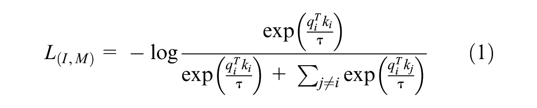
L_{(I, M)} = - \log \frac{\exp (\frac{q_{i}^{T} k_{i}}{τ})}{\exp (\frac{q_{i}^{T} k_{i}}{τ}) + \sum_{j \neq i} \exp (\frac{q_{i}^{T} k_{j}}{τ})}

(1)

where τ is a scalar temperature value that regulates the SoftMax distribution smoothness and j refers to all observations unrelated to i. In every mini-batch, it is considered negative for every observation j $\neq i$ . In training, the symmetric losses L_(I,M) and L_(I,M) are used. The calculation of this loss makes it such that the embeddings q_i and k_i become closer in the embedding space. Even though the training is done on image pairs (I,M1) and (I,M2) for the different modalities, an emergent behavior where modalities (M1,M2) are also aligned in the embedding space is observed.

Dimensionality Reduction and Embedding Clustering

The output of the ViT, a 1024-dimensional vector, is reduced to a 2D vector to enable visualization and clustering of image embeddings. To preserve the discriminative features of the images in two dimensions, t-SNE (t-distributed stochastic neighbor embedding) ( 45 ) was used for dimensionality reduction. It computes conditional probabilities by mapping the pairwise similarities between data points in the high- and lower-dimensional space. The conditional probability for point i relative to point j in the high-dimensional space is given by the following:

P_{ij} = \frac{\exp (- \frac{{| | x_{i} - x_{k} | |}^{2}}{2 σ_{i}^{2}})}{\sum_{k \neq j} \exp (- \frac{{| | x_{i} - x_{k} | |}^{2}}{2 σ_{i}^{2}})}

(2)

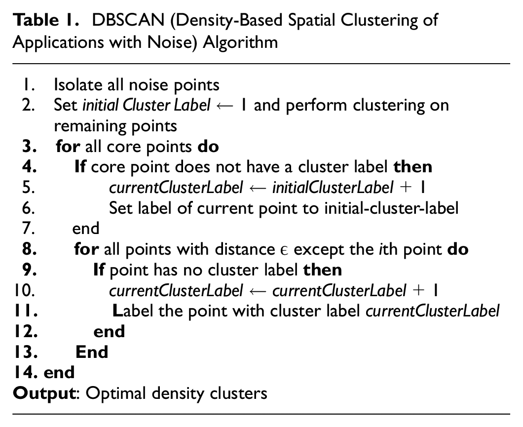
where ∥x_i−x_j∥ represents the Euclidean distance between points i and j in the high-dimensional space and σ_i is the variance of the Gaussian distribution for point i, which can be chosen based on a perplexity value. The conditional probability for the lower-dimensional space is similarly calculated as q_ij. The t-SNE loss function reduces the divergence between these probability distributions using gradient descent to display patterns and relationships that may not be apparent in high-dimensional spaces. t-SNE can assist in recognizing areas of uncertainty in the embedding space, ultimately influencing the selection of informative samples for the AL procedure. The 2D embeddings are subsequently clustered using the density-based spatial clustering of applications with noise (DBSCAN) ( 46 ) algorithm summarized in Table 1. The clustered embeddings and representative images within each cluster are shown in Figure 4. The ×1 and ×2 values in Figure 4 represent the 2D reduced features obtained using t-SNE for the embeddings of each image in our dataset. These values are the coordinates of each data point in the 2D space after dimensionality reduction. The specific range depends on the dataset and the distribution of the embeddings. The ×1 range is (−114.534, 108.0037) and the ×2 range is (−108.116, 112.1794). As shown, the clusters were able to group images based on the camera view angle, time of day, weather condition, dominant class of vehicles, and so forth.

Table 1.

DBSCAN (Density-Based Spatial Clustering of Applications with Noise) Algorithm

01. Isolate all noise points
02. Set

initial Cluster Label \leftarrow 1

and perform clustering on remaining points
03. for all core points do
04. If core point does not have a cluster label then
05.

currentClusterLabel \leftarrow initialClusterLabel + 1

06. Set label of current point to initial-cluster-label
07. end
08. for all points with distance

ϵ

except the

i th

point do
09. If point has no cluster label then
10.

currentClusterLabel \leftarrow currentClusterLabel + 1

11. Label the point with cluster label currentClusterLabel
12. end
13. End
14. end

Output: Optimal density clusters

Figure 4.

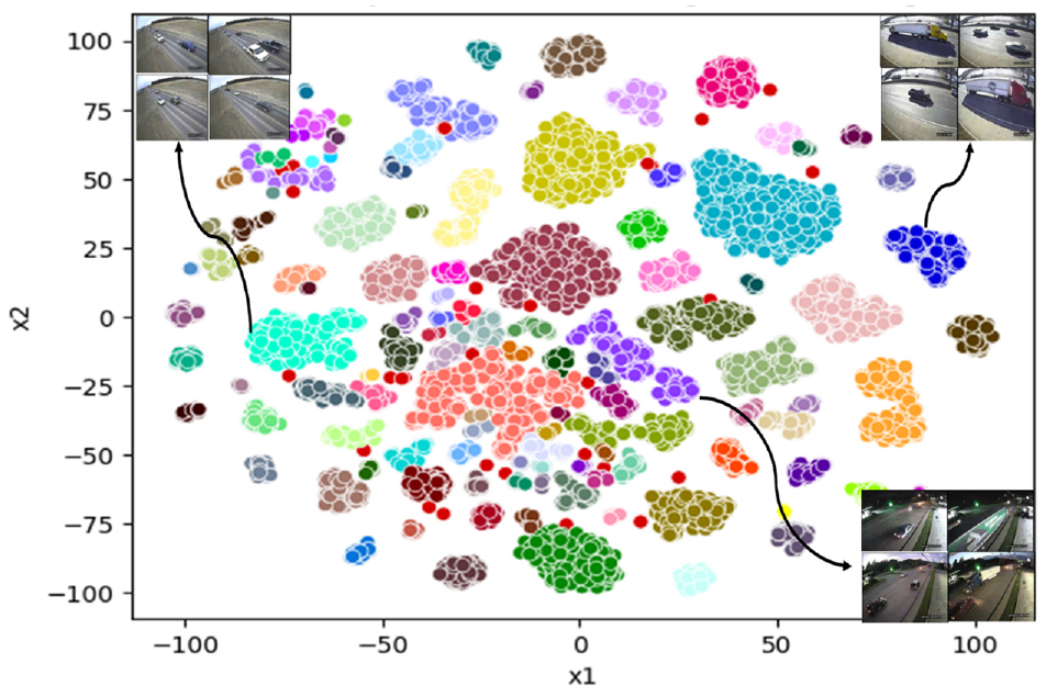
Clustered two-dimensional embeddings of images in our unlabeled data pool.

Image Scoring

Images are scored based on two techniques: a class imbalance score, which reflects the variety of object classes in an image, and a model uncertainty score, which is a measure of how well the learner is able to recognize all objects in an image. Only images with high class imbalance and uncertainty scores are annotated for AL.

The class imbalance score is designed by Equation 3. It prioritizes images with instances from multiple classes. An image with equal instances of all classes will have the highest score. A minimum score is assigned if an image consists of only instances from the majority class:

C I_{score} = Π [1 - \frac{# I_{cls}}{# T_{cls}}]

(3)

The class imbalance score CI of an image is represented by the element-wise multiplication of all the class weights in that specific image.

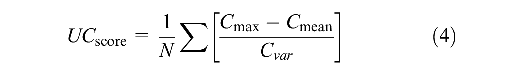
The uncertainty score, designated by Equation 4, is based on model confidence scores assigned to each bounding box by the learner. The confidence score represents the model’s certainty that the predicted object is in the bounding box and belongs to the predicted class. The proposed uncertainty estimation score method for a given image is computed by taking the mean of the absolute value of the difference between the maximum confidence value ( $C_{\max}$ ) and the mean of all the confidence values ( $C_{mean}$ ) and dividing it by the variance of the confidence values ( $C_{var}$ ):

U C_{score} = \frac{1}{N} \sum [\frac{C_{\max} - C_{mean}}{C_{var}}]

(4)

Sampling Strategy—Implementation Details

The study investigates four main sampling strategies: embedding space-guided random sampling, uncertainty score-based sampling, class imbalance score-based sampling, and random sampling without embedding space. The iterative process of sampling, annotating, and model training is described as follows.

Start: Initialize with 100 images randomly sampled from the training database. This applied to all sampling techniques.

Learn: Train learner with initial samples for 30 epochs.

Test: Evaluate model on the test data, predict the cluster of images where the model was uncertain or had a low class imbalance score. We use cosine similarity between the embedding of the test image and the embeddings of the training images to determine which cluster a test image will belong to.

Sample: Sample a new set of images from the unlabeled pool images with similar cluster labels as those predicted in the previous step.

Retrain: Add new samples to the initial samples and retrain.

Iterate: Repeat steps 2–4 until uncertainty scores at step 3 converge. In the current study we constrained the process to only three iterations.

Active Learner

The scoring and sampling strategies are used to select informative images from the embedding space, which are labeled and added to the existing labeled set. These selected images are subsequently passed on to the active learner, YOLOv8 ( 47 ), recently released by Ultralytics. YOLOv8 is the newest version of the YOLO series and a cutting-edge single-stage object detection model. The general structure of YOLOv8 is illustrated in Figure 5. It consists of two main components: the backbone and head. The backbone consists of a series of convolutional and C2f blocks that bundles and forms representational image features at contrasting granularities. The C2f block contains convolutional and bottleneck modules that merge high-level features containing contextual information, improving performance. The SPPF block, attached as YOLO’s final backbone block, pools different features, therefore speeding up computation. The head uses features extracted by the backbone, through a combination of convolutional, C2f, and up-sampling layers, and obtains the box and class prediction functionality. The backbone contains 29 convolutional layers of 3 × 3, receptive field size of 640 × 640, and altogether 27.6 M parameters. YOLOv8 significantly enhances model efficiency and performance by using features such as anchor-free detection, mosaic augmentation, reduced parameter count, the weighted-residual connections, cross mini-batches, normalization, and self-adversarial training. In this study, the YOLOv8 model was trained using the PyTorch ( 48 ) framework. To further optimize vehicle detection, tracking, and counting, the YOLOv8 model is fine-tuned by regulating the subsequent hyperparameters: a batch-size of 64, an optimizer weight decay value of 0.0005, an initial learning rate at 0.01, and a momentum at 0.937 ( 49 ).

Figure 5.

YOLOv8 model structure ( 41 ).

Experiment and Results

The AL methodology developed was validated through a series of experiments. This section describes the datasets used, the different experiments for evaluating the model generalization, and directional traffic count accuracy.

Data Settings

Experiments were conducted using diverse image datasets capturing traffic scenes from freeways and non-freeways, at various camera angles, resolutions, periods, and weather conditions. The datasets were sourced from different agencies including Iowa, Missouri, and Kansas Department of Transportation (DOT) CCTV cameras and 511 Virginia, Dubuque, and St Louis City camera databases from December 2020 to March 2021 ( 50 ). Other publicly available datasets from the AI CITY challenge ( 51 ) and MIO-TCD ( 52 ) were also used. A total of 40,000 images were annotated for model development and the experiments conducted in the following sections. Vehicles were classified according to the Federal Highway Administration (FHWA) scheme. However, some of the classes in the FHWA scheme had to be merged because of the subtle differences between them that could not be visually differentiated with a video because of the camera position. Table 2 shows the differences between the FHWA classification and the classification system used in this paper.

Table 2.

Differences between the Federal Highway Administration (FHWA) Classification and the Classification Adopted in this Paper

FHWA classification scheme	Proposed vision classification scheme
	Class 0: Pedestrians
	Class 00: Cyclists
Class 1: Motorcycles	Class 1: Motorcycles
Class 2: Passenger cars	Class 2: Passenger cars, pickups, and vans
Class 3: Pickups and vans
Class 4: Buses	Class 4: Buses
Class 5: Single-unit, 2-axle trucks	Class 5: Single-unit trucks
Class 6: Single-unit, 3-axle trucks
Class 7: Single-unit, 4-axle trucks
Class 8: Single-trailer, 3- or 4-axle trucks	Class 6: Single-trailer trucks
Class 9: Single-trailer, 5-axle trucks
Class 10: Single-trailer, 6-axle trucks
Class 11: Multi-trailer, 5-axle trucks	Class 7: Multi-trailer trucks
Class 12: Multi-trailer, 6-axle trucks
Class 13: Multi-trailer, 7- or more axle trucks

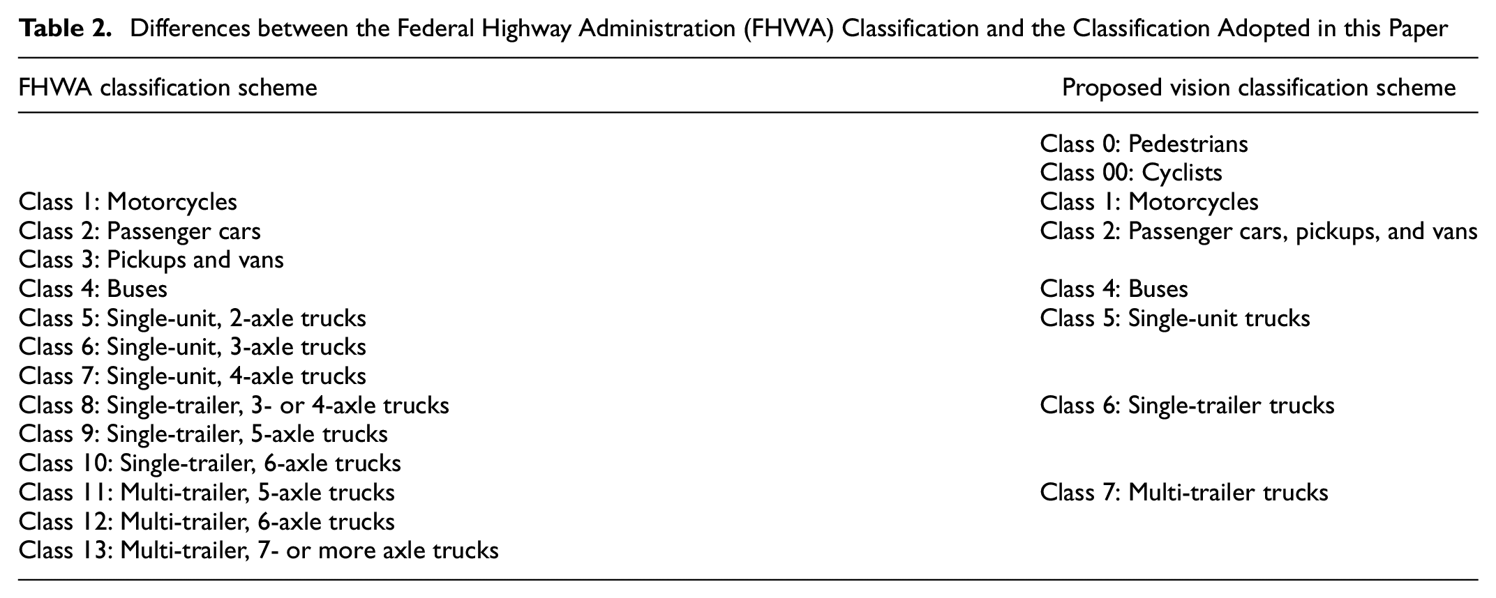
The data collected were divided into unlabeled (75%) and labeled data pools (25%). The labeled data pool had annotations that were used purely for testing model performance. The training and validation datasets were sampled and annotated from the unlabeled data pool. While all the images in the unlabeled pool were eventually annotated, the experiments below show that only about 30% of the unlabeled pool should have been annotated to achieve state-of-the-art performance.

Evaluation Metric

The mean average precision (mAP) leverages sub-metrics, including the confusion matrix, intersection over union (IoU), precision, and recall, giving a more robust performance measure for object detection models. The mAP is computed by finding the average of the average precision, which is the area under the precision recall curve. It ranges from 0 to 1, with 1 being the highest. The formula for the mAP is given in Equation 5, where APk is the AP of class k, and n is the number of classes:

mAP = \frac{1}{n} \sum_{k = 1}^{k = n} A P_{k}

(5)

Baseline Model Settings

All experiments conducted in this section are compared to a baseline YOLOv8 model. The model was trained for 30 epochs on all images in the “unlabeled” data pool. There were about 600,000 instances of passenger cars, 125,000 instances of single-units and trucks, and 8000 instances of pedestrian, cyclists, and motorcycles. The model was trained using the default configuration settings of the YOLOv8 architecture. The default configuration setting for the training utilized the “yolov8n.pt” pre-trained model, an input image size of 640 × 640, the default Compute Unified Device Architecture (CUDA) device, and the “auto” optimizer option. The “auto” optimizer option automatically selects an appropriate optimization algorithm and its hyperparameters based on the specific model architecture and problem being solved. The available optimizer options include SGD (stochastic gradient descent), Adam, Adamax, AdamW, NAdam, RAdam, RMSProp, and “auto.” This dynamic selection relieves the user from the manual task of choosing an optimizer, ensuring that the training process is optimized effectively. To ensure reproducibility, a random seed of 0 was set. Notably, none of the layers were frozen, and dropout regularization was disabled.

Inference Performance on a Central Processing Unit and Graphics Processing Unit

In our study, the central processing unit (CPU) utilized was a 13th Gen Intel Core (TM) i9-13900HX, while the graphics processing unit (GPU) was an NVIDIA GeForce RTX 4080 Laptop GPU with 12010MiB. Table 3 provides insight into the CPU and GPU inference times per image in milliseconds (ms) and frames per second (fps). The observed results reveal consistent GPU inference times across all models, showcasing uniform efficiency. As expected, CPU inference times are generally lower than GPU times, a notable feat considering the impressive real-time performance even on the CPU. Notably, the CI_US and EMB_RAND strategies exhibit higher fps than the fully trained model, indicating their potential for real-time applications. The comparable inference times between the GPU and CPU, coupled with the impressive fps metrics, underscore the practicality of our model for real-time applications, even on resource-constrained CPUs. These findings highlight the versatility and efficiency of our proposed AL framework in diverse computing environments.

Table 3.

Inference Times for Active Learning Strategies on the Central Processing Unit (CPU) and Graphics Processing Unit (GPU)

	CPU inference per image (ms)	GPU inference per image (ms)	CPU inference per image (fps)	GPU inference per image (fps)
Full	15.1	0.9	66	1111
CI	17.0	0.9	59	1111
CI_US	14.2	0.9	70	1111
EMB_RAND	14.8	0.9	68	1111

Note: CI = models trained with class imbalance scoring and sampling; CI-US = models trained with images sampled using both class imbalance and model uncertainty sampling; EMB-RAND = purely random sampling from the clustered embedding space; fps = frames per second.

An In-Depth Exploration of Fixed and Adaptive Training Epochs

In this section, we delve into a nuanced analysis of fixed and adaptive training epochs. For the full training dataset, we conducted experiments using both fixed epochs (30 epochs, as employed in the study) and adaptive epochs determined by early stopping with a patience of 40 epochs, resulting in convergence at 129 epochs. The subsequent evaluation on unseen data, distinct from the training set, revealed that the model trained on variable epochs did not exhibit superior performance across all classes compared to its fixed-epoch counterpart. As shown in Figure 6, both models had the same mAP for the cyclist, car, and bus classes. The mAP values for the remaining classes demonstrated a striking similarity between the two models. This observation prompts a crucial consideration that the pursuit of convergence through a higher number of epochs does not necessarily guarantee improved model performance. Overfitting, a potential consequence of prolonged training, underscores the complexity of the convergence-performance trade-off. Our findings underscore the need for a nuanced understanding of convergence dynamics and caution against relying solely on training until convergence as a metric for model superiority. In conclusion, we made a deliberate decision to employ a fixed 30 epochs, aiming to strike a judicious balance between effective utilization of computational resources and efficient training time.

Figure 6.

Comparison of fixed epochs and variable epochs for models trained on the full dataset.

Yolov8 relies on three pivotal loss functions, namely classification loss for accurate object class labeling, box loss for precise object localization, and distribution focal loss (DFL) to tackle class imbalance. Our decision to adhere to a fixed 30 epochs is substantiated by the inclusion of visualizations depicting validation losses and mAP50, as shown in Figure 7. On scrutinizing the validation loss and mAP50 plot, distinct convergence patterns emerged. Notably, by the 30-epoch mark, the model displayed signs of convergence, and there was minimal disparity in losses between 30 and 129 epochs. This observation underscores the efficiency of the model’s learning process within the chosen epoch range. Given the modest size of our dataset, we consciously opted for 30 epochs to mitigate potential overfitting risks. The rationale behind this decision lies in the delicate balance between maximizing computational resources and ensuring the model’s effectiveness. By selecting a conservative epoch count, we aimed to strike this balance, prioritizing generalization over memorization, and emphasizing the pragmatic utilization of resources for optimal model performance.

Figure 7.

Validation loss plot and mAP50 metric plot for fully trained models.

Influence of Scoring and Sampling Strategies in Embedding Space

As discussed in the preceding sections, there were three scoring and sampling techniques used to select the most informative, diverse, and balanced images for the active learner. This section uses the mAP metric to evaluate the effectiveness of these techniques, comparing them to the baseline model. Figure 8 shows the performance of the different strategies across all seven classes of vehicles. CI represents models trained with class imbalance scoring and sampling, CI-US models were trained with images sampled using both class imbalance and model uncertainty sampling, and EMB-RAND is purely random sampling from the clustered embedding space. The x-axis of the plot shows the number of sampled images expressed as a percentage of the images used to train the baseline model.

Figure 8.

Comparison of different scoring and sampling techniques against the baseline model at varying sampling rates.

It can be observed from the figure that increasing the sampling rate generally leads to higher mAP for all techniques. At 30% sampling rate, all active learner models yielded comparable mAP to the base model. For cyclists, buses, and trucks, all models trained using the proposed sampling techniques performed better (at only 30% sampling rate) than the baseline model with between 8% and 20% mAP gain. This observation suggests that utilizing the entire dataset for training may not always yield optimal results for certain classes. Some images have a degrading effect on model accuracy and therefore it is necessary to implement strategies that can select the most informative and diverse images for training. The baseline model, however, maintained significantly higher mAP for pedestrians and single-unit trucks with about 25% mAP gain. It should be noted that the baseline model was trained with more than 2000 instances of pedestrians and 12,000 instances of single-unit trucks. Our sampling technique could only select about 5% of these instances (although 30% of the data was used) because of the lack of diversity in traffic scenes where pedestrians and single-unit trucks were captured. From a total of 51 clusters in the embedding space, pedestrians and single-unit trucks were found in only eight clusters. This limited the sampling scope and therefore resulted in low sampling rates for these classes. Of the three sampling techniques, CI-US had the highest mAP on average, for low sampling rates. At the 30% sampling rate, random sampling, which consistently had the lowest mAP at low sampling rates, edges slightly above the other models. The influence of the embedding space dominates that of the scoring techniques at the 30% sampling rate and, as a result, random sampling may be sufficient when the percentage of data used is significantly increased.

Influence of Embedding Space

The 2D clustered embedding space is a key component of the proposed AL framework developed. To evaluate its influence on the active learner, two models were trained: the first model is trained with 500, 1000, 1500, 3000, and 6000 images randomly sampled from our unlabeled pool. A second model is trained using the same sampling rate; however, the selection of the samples was guided by the clustered embeddings. The number of samples from a cluster is weighted by the size of the cluster. Figure 9 shows the remarkable influence of sampling from the embedding space. From the figure, although the mAP values seem to be converging with increasing sampling rates, embedding-guided random sampling yields a significantly higher mAP. Sampling from the embedding space increases the likelihood of having a more diverse dataset for training. Therefore, there is an improvement in model performance.

Figure 9.

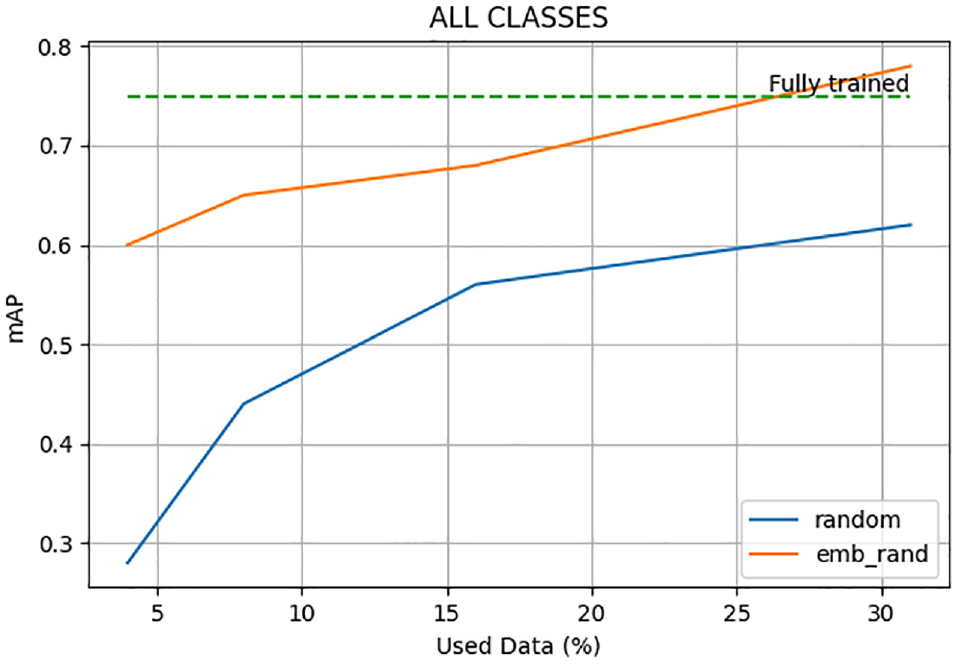
Comparison of random sampling and embedding space-guided random sampling against the baseline model at varying sampling rates.

Model Generalization

In general, models trained on very large datasets are able to adapt properly to new, previously unseen data. In this section, we compare models trained using the AL method proposed to models trained on the full dataset with respect to generalizability. This test was conducted using images captured from cameras whose perspective, height, and resolution were significantly different from the data used to train the models. Figure 10 shows the cluster locations of these images in the 2D embedding space. As observed, their clustered embeddings are significantly different from other clusters and therefore a good test for model transferability or generalization.

Figure 10.

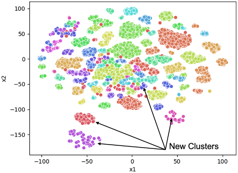
Clustering embeddings of images used to test generalizability of the active learning framework developed.

A visualization of the number of false positives, false negatives, and true positives per pixel is used to evaluate the performance of the AL pipeline developed. These accuracy measures were subsequently projected spatially for visual and qualitative evaluation of the model’s ability to generalize on new data. Figures 11 –13 compare CI-US and the baseline model under varying conditions. The first row in all the figures show the results from the AL model (CI-US). The first, second, and third columns shows the spatial count of false negatives, false positives, and true positives, respectively. For a well-generalized model, the heatmap in the third column should be more pronounced compared to those in the first and second columns. For the high-volume intersection with a distant camera in Figure 11, most of the false positives and false negatives were observed in the parking lots and for vehicles that were not close to the intersection. There is a high concentration of true positives in the intersection, which is generally a good trend. Both models had similar heatmaps, although the intensity of false positives and false negatives for the AL model is slightly lower than that of the baseline model. Similar trends can be observed from Figure 12, where the models were tested under snow conditions. Under the night condition shown in Figure 13, there was a significant difference in generalizability for both models. While our training dataset had images captured under night conditions, most were not from congested scenes. The AL model completely failed to detect vehicles in the southbound direction, as shown in the true positive heatmap. The baseline model was able to detect a fraction of vehicles in the southbound direction; however, this led to significantly high false positives in that direction. In such cases where traffic conditions are significantly different from the data used to train models, AL-based models are more likely to have more false negatives than false positives.

Figure 11.

Heatmap of accuracy measures for a high-volume intersection more than 125 ft from the camera location. The first row represents outputs from the active learning model and the second row represents outputs from the full model. First column—false negatives, second column—false positives, and third column—true positives.

Figure 12.

Heatmap of accuracy measures for a high-volume freeway under snow conditions. Localized false positives and negatives at distant locations from the camera. The intensity of the true positive heatmap is considerably higher.

Figure 13.

Heatmap of accuracy measures for a high-volume freeway under night conditions. Models failed to generalize, as the intensity of the true positive, false positive, and false negative heatmaps are comparable.

It is important to note that the challenge of false negatives and false positives is not limited to AL models but also affects fully trained models. To mitigate the issue of increased false negatives, a practical approach involves the diversification of the training data. While our experimental setup intentionally excluded training on images related to the generalizability testing images for research purposes, real-world applications benefit from diversifying the training dataset to encompass scenarios closely resembling the challenging test images. This diversification strategy exposes the model to a broader spectrum of conditions during training, thereby enhancing its adaptability to novel scenarios and reducing the occurrence of false negatives. The incorporation of diverse training data is a valuable measure for bolstering model generalization, particularly in cases where traffic conditions significantly deviate from the data used for training.

Traffic Count Accuracy

Lastly, we evaluate the accuracy of the AL models developed for obtaining directional traffic counts at intersections and on freeways. Vision-based traffic counts typically involve three main steps: object recognition, object tracking, and clustering for directional counts. In this study, object recognition is carried out using the AL models developed in the preceding sections. The outputs from the recognition model are fed into an object tracker that associates each object with a unique identification from one frame to the other. The study used ByteTrack ( 53 ) for object tracking. ByteTrack tracks objects by associating all detection boxes instead of only using detections with high confidence scores. This is the key difference between ByteTrack over other tracking methods ( 54 , 55 ). In Figure 14, we show sample trajectories generated with ByteTrack for different intersections and freeways. Clustering algorithms using functions such as cosine similarity can be used to group and count these trajectories by direction, as shown in Figure 14.

Figure 14.

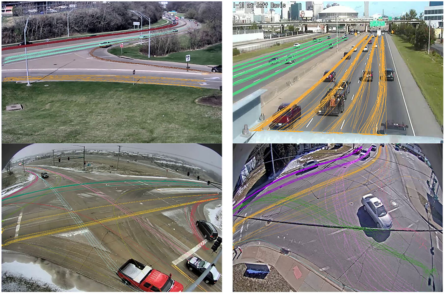
Vehicle tracking for directional traffic counts on intersections and freeways.

We use box-and-whisker plots to depict a concise and informative summary of vehicle count accuracy distributions, including central tendency, variability, and outliers. On examining the box-and-whisker plot in Figure 15, it becomes evident that our proposed model CI-US yields comparable results to the fully trained model when evaluating the accuracy of vehicle counts. However, it is worth noting that while the EMB-RAND surpassed CI-US and CI in the latter AL cycles for object detection, they did not outperform CI-US in vehicle counting. Therefore, in practical scenarios where vehicle counting is a priority and the cost and time of annotation must be minimized, CI-US should emerge as the most favorable choice.

Figure 15.

Comparison of vehicle count accuracy of the proposed models and the baseline model.

To estimate count accuracy, we manually counted directional movements from 5-min videos collected at different intersections and freeways and in different weather conditions. A comparison of CI-US model counts against the ground truth is shown in Table 4. The results show that the CI-US model performs relatively well when compared to the ground truth.

Table 4.

CI-US Model Directional Freeway and Intersection Vehicle Counts Against the Ground Truth

Freeways	North bound		Accuracy	South bound		Accuracy
Video 1	101/113		89.4	115/124		92.7
Video 2	76/95		80	107/150		71.3
CCTV	91/96		94.8	48/105		45.7
Intersections	Through	Accuracy	Right	Accuracy	Left	Accuracy
Video 3	32/36	88.9	19/22	86.4	6/6	100
Video 4	34/96	35.4	7/13	53.8	6/9	66.7
Video 5	62/67	92.5	9/1	22.5	41/48	85.4
Video 6	62/64	96.9	7/7	100	18/19	94.7
Video 7	45/52	86.5	4/7	92.3	3/5	60
Video 8	19/32	59.4	7/8	93.8	3/14	21.4

Note: CI-US = models trained with images sampled using both class imbalance and model uncertainty sampling; CCTV = closed circuit television.

Discussion and Conclusions

The paper presents a novel AL framework designed to significantly reduce the number of annotation labels required for training a vehicle detection and classification model. The AL framework is based on the generation of image embeddings through a ViT network. The generated embeddings are subsequently clustered and projected to a lower-dimensional space using t-SNE to ease sampling. Following this, image scores based on the class imbalance (CI) and uncertainty score (US) are further calculated to supplement the sampling of images to be labeled. An iterative sampling strategy is suggested with four main sampling strategies being investigated: embedding space-guided random sampling, uncertainty score-based sampling, class imbalance score-based sampling, and random sampling without embedding space.

The proposed AL strategy is tested on YOLOv8 using images captured representing traffic scenes from freeways and non-freeways and compared against a baseline trained on all available data. The active learner model outperformed the baseline model with only 30% of the data used to train the baseline model. This observation suggests that utilizing the entire dataset may not always yield optimal results for certain classes. Of the sampling techniques, CI-US had the highest mAP on average, for low sampling rates. At a 30% sampling rate, embedding-guided random sampling, which consistently had the lowest mAP, edges slightly above the other models. With respect to model transferability, the YOLOv8 active learner was able to adapt to new, previously unseen data. The learner was also able to accurately count vehicles by direction at a rate comparable to the baseline model.

The practical use of the framework proposed includes the following: selecting which images should be annotated, thus saving manual annotation time and reducing the effect of class imbalance on developed models. The framework could also be used to pre-determine whether a developed model will be able to process a traffic video accurately or not. Videos flagged as not suitable for a developed model can be sampled and added to training data for model retraining.

Owing to the large potential of AL, the proposed framework can be adopted in different computer vision tasks, such as object recognition in self-driving cars, traffic management, and vehicle tracking. Despite its numerous advantages, the proposed AL method is limited in that where traffic conditions were significantly different from the data used to train the models, the AL-based model was more likely to have more false negatives than false positives. Future studies should look at applying AL for other vision tasks, such as segmentation, key point detection, and tracking.

Footnotes

Author Contributions

The authors confirm contribution to the paper as follows: study conception and design: Y. Adu-Gyamfi; data collection: Y. Adu-Gyamfi; analysis and interpretation of results: E. Arthur, Y. Adu-Gyamfi; draft manuscript preparation: E. Arthur, T. Muturi, Y. Adu-Gyamfi. All authors reviewed the results and approved the final version of the manuscript.

Declaration of Conflicting Interests

The author(s) declared no potential conflicts of interest with respect to the research, authorship, and/or publication of this article.

Funding

The author(s) disclosed receipt of the following financial support for the research, authorship, and/or publication of this article: The National Science Foundation under grant award number 2045786.

ORCID iDs

Elizabeth Arthur

Tanner Muturi

Yaw Adu-Gyamfi

References

Zhuang

Duan

Zhu

Xiong

A Comprehensive Survey on Transfer Learning. Proceedings of the IEEE, Vol. 109, No. 1, 2020, pp. 43–76.

Langnickel

Fluck

We Are Not Ready Yet: Limitations of Transfer Learning for Disease Named Entity Recognition. bioRxiv, 2021, pp. 2021–2027. i: https://doi.org/10.1101/2021.07.11.451939.

Williams

Tadesse

Sam

Sun

Montañez

G. D.

Limits of Transfer Learning. In Machine Learning, Optimization, and Data Science ( Nicosia

Ojha

La Malfa

Jansen

Sciacca

Pardalos

Giuffrida

Umeton

, eds.), Springer International Publishing, Cham, Switzerland, pp. 382–393.

Vinyals

Blundell

Lillicrap

Wierstra

Matching Networks for One Shot Learning. Advances in Neural Information Processing Systems, Vol. 29, 2016.

Parnami

Lee

Learning from Few Examples: A Summary of Approaches to Few-Shot Learning. http://arxiv.org/abs/2203.04291. Accessed October 18, 2023.

H.-J.

Ming

Zhan

D.-C.

Chao

W.-L.

Few-Shot Learning with a Strong Teacher. IEEE Transactions on Pattern Analysis and Machine Intelligence, Vol. 46, No. 3, 2024, pp. 1425–1440.

Socher

Ganjoo

Manning

C. D.

Zero-Shot Learning through Cross-Modal Transfer. Advances in Neural Information Processing Systems, Vol. 26, 2013.

Dandu

Sharma

Bhandarkar

S. M.

Exploring the Limits of Zero-Shot Learning-How Low Can You Go?

Proc., IEEE/CVF Conference on Computer Vision and Pattern Recognition Workshops (CVPRW), Nashville, TN, IEEE, New York, 2021.

Xian

Schiele

Akata

Zero-Shot Learning-the Good, the Bad and the Ugly. Proc., IEEE Conference on Computer Vision and Pattern Recognition (CVPR), Honolulu, HI, IEEE, New York, 2017.

10.

Angluin

Queries and Concept Learning. Machine Learning, Vol. 2, No. 4, 1988, pp. 319–342. https://doi.org/10.1023/A:1022821128753.

11.

Dagan

Engelson

S. P.

Committee-Based Sampling for Training Probabilistic Classifiers. Proc., Machine Learning Proceedings 1995: Proceedings of the Twelfth International Conference on Machine Learning, Tahoe City, CA, July 9–12, 1995, Elsevier, Amsterdam, Netherlands, pp. 150–157.

12.

Lewis

D. D.

A Sequential Algorithm for Training Text Classifiers: Corrigendum and Additional Data. ACM SIGIR Forum, Vol. 29, No. 2, 1995, pp. 13–19. https://doi.org/10.1145/219587.219592.

13.

Krishnakumar

Active Learning Literature Survey. Technical Reports. University of California, Santa Cruz, Vol. 42, 2007.

14.

Vahdat

Belbahri

Nia

V. P.

Active Learning for High-Dimensional Binary Features. Proc., 15th International Conference on Network and Service Management (CNSM), Halifax, Canada, IEEE, New York, 2019.

15.

Caron

Heskes

Otten

Stienen

Constraining the Parameters of High-Dimensional Models with Active Learning. The European Physical Journal C, Vol. 79, No. 11, 2019, p. 944. https://doi.org/10.1140/epjc/s10052-019-7437-5.

16.

Khalifa

O. O.

Wajdi

M. H.

Saeed

R. A.

Hashim

A. H. A.

Ahmed

M. Z.

Ali

E. S.

Vehicle Detection for Vision-Based Intelligent Transportation Systems Using Convolutional Neural Network Algorithm. Journal of Advanced Transportation, Vol. 2022, 2022, p. e9189600. https://doi.org/10.1155/2022/9189600.

17.

Farid

Hussain

Khan

Shahzad

Khan

Mahmood

A Fast and Accurate Real-Time Vehicle Detection Method Using Deep Learning for Unconstrained Environments. Applied Sciences, Vol. 13, No. 5, 2023, p. 3059. https://doi.org/10.3390/app13053059.

18.

Zhang

Guo

Tian

Tang

Guo

Real-Time Vehicle Detection Based on Improved YOLO V5. Sustainability, Vol. 14, No. 19, 2022, p. 12274. https://doi.org/10.3390/su141912274.

19.

Nguyen

Deep Neural Network-Based Detection of Road Traffic Objects from Drone-Captured Imagery Focusing on Road Regions. International Journal of Advanced Computer Science and Applications, Vol. 14, No. 9, 2023. https://doi.org/10.14569/IJACSA.2023.0140933, pp. 307–314.

20.

Yan

Liu

Wang

Yue

Wang

LOVD: Land Vehicle Detection in Complex Scenes of Optical Remote Sensing Image. IEEE Transactions on Geoscience and Remote Sensing, Vol. 60, 2022, pp. 1–13. https://doi.org/10.1109/TGRS.2021.3133109.

21.

Käding

Rodner

Freytag

Denzler

Fine-Tuning Deep Neural Networks in Continuous Learning Scenarios. In Computer Vision – ACCV 2016 Workshops ( Chen

C.-S.

K.-K.

, eds.), Springer International Publishing, Cham, Switzerland, pp. 588–605.

22.

Wang

Shang

A New Active Labeling Method for Deep Learning. Proc., International Joint Conference on Neural Networks (IJCNN), Beijing, China, IEEE, New York, 2014.

23.

Roth

Small

Margin-Based Active Learning for Structured Output Spaces. In Machine Learning: ECML 2006 ( Fürnkranz

Scheffer

Spiliopoulou

, eds.), Springer, Heidelberg, Berlin, pp. 413–424.

24.

Joshi

A. J.

Porikli

Papanikolopoulos

Multi-Class Active Learning for Image Classification. Proc., IEEE Conference on Computer Vision and Pattern Recognition, Miami, FL, IEEE, New York, 2009.

25.

Wang

Zhang

Lin

Cost-Effective Active Learning for Deep Image Classification. IEEE Transactions on Circuits and Systems for Video Technology, Vol. 27, No. 12, 2016, pp. 2591–2600.

26.

Bietti

Active Learning for Object Detection on Satellite Images. Technical Report. Caltech, Pasadena, CA, 2012.

27.

Vijayanarasimhan

Grauman

Large-Scale Live Active Learning: Training Object Detectors with Crawled Data and Crowds. International Journal of Computer Vision, Vol. 108, No. 1–2, 2014, pp. 97–114. https://doi.org/10.1007/s11263-014-0721-9.

28.

Stark

Hazırbas

Triebel

Cremers

CAPTCHA Recognition with Active Deep Learning. https://cvg.cit.tum.de/_media/spezial/bib/stark-gcpr15.pdf.

29.

Holub

Perona

Burl

M. C.

Entropy-Based Active Learning for Object Recognition. Proc., IEEE Computer Society Conference on Computer Vision and Pattern Recognition Workshops, Anchorage, AK, IEEE, New York, 2008.

30.

Haussmann

Fenzi

Chitta

Ivanecky

Roy

Mittel

Koumchatzky

Farabet

Alvarez

J. M.

Scalable Active Learning for Object Detection. Proc., IEEE Intelligent Vehicles Symposium (IV), Las Vegas, NV, IEEE, New York, 2020.

31.

Liang

Deng

Cai

Jiang

Jia

Exploring Diversity-Based Active Learning for 3D Object Detection in Autonomous Driving. http://arxiv.org/abs/2205.07708. Accessed November 2, 2023.

32.

Sinha

Ebrahimi

Darrell

Variational Adversarial Active Learning. Proc., IEEE/CVF International Conference on Computer Vision (ICCV), Seoul, Korea (South), IEEE, New York, 2019.

33.

Zhdanov

. Diverse Mini-Batch Active Learning. http://arxiv.org/abs/1901.05954. Accessed November 2, 2023.

34.

Prabhu

Chandrasekaran

Saenko

Hoffman

Active Domain Adaptation via Clustering Uncertainty-Weighted Embeddings. Proc., IEEE/CVF International Conference on Computer Vision (ICCV), Montreal, Canada, 2021.

35.

Sener

Savarese

Active Learning for Convolutional Neural Networks: A Core-Set Approach. http://arxiv.org/abs/1708.00489. Accessed October 18, 2023.

36.

Agarwal

Arora

Anand

Arora

Contextual Diversity for Active Learning. In Computer Vision – ECCV 2020 ( Vedaldi

Bischof

Brox

Frahm

J.-M.

, eds.), Springer International Publishing, Cham, Switzerland, pp. 137–153.

37.

Gkelios

Kastellos

Boutalis

Chatzichristofis

S. A.

Universal Image Embedding: Retaining and Expanding Knowledge with Multi-Domain Fine-Tuning. IEEE Access, Vol. 11, 2023, pp. 38208–38217.

38.

Girdhar

El-Nouby

Liu

Singh

Alwala

K. V.

Joulin

Misra

Imagebind: One Embedding Space to Bind Them All. Proc., IEEE/CVF Conference on Computer Vision and Pattern Recognition (CVPR), Vancouver, Canada, IEEE, New York, 2023.

39.

Vaswani

Shazeer

Parmar

Uszkoreit

Jones

Gomez

A. N.

Kaiser

Ł.

Polosukhin

Attention is All You Need. Advances in Neural Information Processing Systems, Vol. 30, 2017.

40.

Dosovitskiy

Beyer

Kolesnikov

Weissenborn

Zhai

Unterthiner

Dehghani

, et al. An Image is Worth 16x16 Words: Transformers for Image Recognition at Scale. http://arxiv.org/abs/2010.11929. Accessed October 18, 2023.

41.

Wang

Xiao

Zhu

Wong

D. F.

Chao

L. S.

Learning Deep Transformer Models for Machine Translation. http://arxiv.org/abs/1906.01787. Accessed October 18, 2023.

42.

Baevski

Schneider

Auli

Vq-Wav2vec: Self-Supervised Learning of Discrete Speech Representations. http://arxiv.org/abs/1910.05453. Accessed October 18, 2023.

43.

Radford

Kim

J. W.

Hallacy

Ramesh

Goh

Agarwal

Sastry

, et al. Learning Transferable Visual Models from Natural Language Supervision. arXiv Preprint arXiv:2103.00020, 2021.

44.

Cherti

Beaumont

Wightman

Wortsman

Ilharco

Gordon

Schuhmann

Schmidt

Jitsev

Reproducible Scaling Laws for Contrastive Language-Image Learning. Proc., IEEE/CVF Conference on Computer Vision and Pattern Recognition (CVPR), Vancouver, Canada, IEEE, New York, 2023.

45.

Van der Maaten

Hinton

Visualizing Data Using T-SNE. Journal of Machine Learning Research, Vol. 9, No. 11, 2008, pp. 2579–2605.

46.

Ester

Kriegel

H.-P.

Sander

A Density-Based Algorithm for Discovering Clusters in Large Spatial Databases with Noise. Proc., KDD-96, 1996, ACM, New York, NY, pp. 226–231.

47.

Ultralytics. YOLOv8. https://docs.ultralytics.com/models/yolov8. Accessed October 22, 2023.

48.

Paszke

Gross

Massa

Lerer

Bradbury

Chanan

Killeen

, et al. Pytorch: An Imperative Style, High-Performance Deep Learning Library. Advances in Neural Information Processing Systems, Vol. 32, 2019, pp. 8024–8035.

49.

Aboah

Shoman

Mandal

Davami

Adu-Gyamfi

Sharma

A Vision-Based System for Traffic Anomaly Detection Using Deep Learning and Decision Trees. Proc., IEEE/CVF Conference on Computer Vision and Pattern Recognition Workshops (CVPRW), Nashville, TN, 2021.

50.

Iowa 511 Travel Information. https://511ia.org/@-94.9603,42.19251,7?show=iowaAppIncident,winterDriving,towingProhibitedReports,weatherRadar. Accessed November 6, 2023.

51.

Naphade

Chang

M.-C.

Sharma

Anastasiu

D. C.

Jagarlamudi

Chakraborty

Huang

, et al. The 2018 Nvidia Ai City Challenge. Proc., IEEE/CVF Conference on Computer Vision and Pattern Recognition Workshops (CVPRW), Salt Lake City, UT, IEEE, New York, 2018.

52.

Luo

Branchaud-Charron

Lemaire

Konrad

Mishra

Achkar

Eichel

Jodoin

P.-M.

MIO-TCD: A New Benchmark Dataset for Vehicle Classification and Localization. IEEE Transactions on Image Processing, Vol. 27, No. 10, 2018, pp. 5129–5141.

53.

Zhang

Sun

Jiang

Weng

Yuan

Luo

Liu

Wang

ByteTrack: Multi-Object Tracking by Associating Every Detection Box. In Computer Vision – ECCV 2022 ( Avidan

Brostow

Cissé

Farinella

G. M.

Hassner

, eds.), Springer Nature Switzerland, Cham, pp. 1–21.

54.

Veeramani

Raymond

J. W.

Chanda

DeepSort: Deep Convolutional Networks for Sorting Haploid Maize Seeds. BMC Bioinformatics, Vol. 19, No. S9, 2018, p. 289. https://doi.org/10.1186/s12859-018-2267-2.

55.

Wojke

Bewley

Paulus

Simple Online and Realtime Tracking with a Deep Association Metric. Proc., IEEE International Conference on Image Processing (ICIP), Beijing, China, IEEE, New York, 2017.