Automatic Detection of Road Subsurface Distress via Curriculum Learning: Learn Like an Expert

Abstract

The application of deep learning algorithms for subsurface distress detection using ground penetrating radar (GPR) data has seen extensive utilization. However, a significant impediment arises because of the challenge in acquiring ground-truth subsurface distress samples. This scarcity of labeled data leads to incomplete training of deep learning algorithms and gives rise to a critical concern with respect to over-fitting. Generating additional samples through numerical simulation constitutes one of the most efficient methods to overcome insufficient GPR training samples. If both real and simulated samples are mixed for training, the deep learning model may miss the complexities in the samples and their learning state. Concurrently, the presence of noise and anomalous samples might lead the model to converge toward a suboptimal local minimum. This phenomenon is particularly conspicuous in the field of GPR because of the stochastic and disordered propagation of radar waves, resulting in amplified noise and abnormal samples. A robust curriculum learning algorithm, inspired by expert training methods, was created to train models from simple simulated samples to complex field samples. This strategy evaluates the performance of two object detection models, YOLOv7 and Faster R-CNN, under the proposed framework. Compared to the model trained from the whole datasets out of order, the precision, recall, F1_score, and mean average precision are all improved. The results demonstrate that the proposed method can enhance the model’s precision by approximately 8% and recall by about 11% under the same dataset. These findings highlight its great potential for expediting convergence and boosting the overall model performance.

Keywords

subsurface distress ground penetrating radar automatic detection curriculum learning deep learning

Accurate detection and timely maintenance of road subsurface distress (RSD) are of paramount importance in extending the long-term service life of road infrastructure ( 1 ). Ground penetrating radar (GPR) has emerged as one of the most widely used techniques owing to its continuous non-destructive nature, rapid speed, high precision, and cost-effectiveness ( 2 ). GPR operates by transmitting high-frequency electromagnetic waves (EWs) into the subsurface via a transmitting antenna. These waves undergo scattering, reflection, transmission, or refraction at interfaces with distinct electrical properties ( 3 ). Subsequently, after a specific period, a portion of the EW returns to the surface and is captured by a receiving antenna. The acquired signals’ propagation time and amplitude intensity are recorded by computer software systems, thereby generating a two-dimensional cross-sectional representation by assigning colors or grayscale to depict the amplitude intensity values ( 4 ). RSD, such as a crack, cavity, or loose base, can be easily detected because a portion of the EW is reflected when it propagates into the location of the distress. Despite the multitude of advantages associated with the GPR technique, distress identification mainly relies on expert interpretation. The efficiency and accuracy of data analysis highly depend on the proficiency of technical personnel. However, when confronted with large datasets, ensuring prompt and precise interpretations becomes an arduous task ( 5 , 6 ). Consequently, the development of robust methodologies for GPR-automated identification of distress assumes critical significance.

With the development of digital signal processing and computer vision, various algorithms for automated identification of RSD using GPR have been proposed. Firstly, algorithms based on EW theory and pattern recognition have been utilized ( 7 ). Linear and hyperbolic features, commonly observed in GPR images, enable the transformation of RSD detection into pattern recognition. Prominent algorithms in this category include the Hough transform, least squares method, edge detection, and shape clustering ( 8 , 9 ). While these algorithms perform well under ideal numerical simulation conditions, in practical field applications, environmental interference affects the Ews, leading to significant distortion of defect morphology. Secondly, traditional machine learning algorithms have been employed for automated RSD detection. This approach typically involves three stages: signal preprocessing, feature extraction, and model training ( 10 ). Signal preprocessing aims to remove noise and enhance target reflections. Feature extraction relies on theoretical knowledge to select representative defect characteristics ( 11 , 12 ). Model training utilizes algorithms to establish a training set by learning from the extracted features. Commonly used algorithms in this category include clustering algorithms ( 13 ), support vector machines ( 14 ), neural networks ( 15 ), k-nearest neighbors ( 16 ), hidden Markov models ( 17 ), and so forth. However, traditional machine learning algorithms require manual feature extraction from GPR signals, and their accuracy heavily relies on the chosen features, limiting their performance to specific datasets. The last one has been the fastest-growing deep learning algorithm in recent years. Compared to traditional machine learning algorithms that rely on manually selecting features, deep learning algorithms demonstrate powerful capabilities in extracting complex features, especially in image-related object recognition tasks ( 18 , 19 ). They can independently extract sample features layer by layer without the need for manual feature extraction or expert knowledge, significantly improving the accuracy and efficiency of GPR target recognition ( 20 ).

Although deep learning models have facilitated the advancement of intelligent recognition in GPR, they have not yet reached the anticipated level of performance ( 21 ). This is primarily because of the requirement of determining a substantial number of weight parameters during model training ( 22 , 23 ). The field data for GPR is challenging to obtain as it is buried underground. In addition, the limited training samples can lead to issues such as unstable model networks, difficulties in decreasing the loss function, and over-fitting. Currently, three main approaches are being employed to address this challenge: (a) transfer learning, which involves transferring pre-trained weights from natural image datasets and fine-tuning the parameters on the GPR dataset, thus enhancing model convergence speed and performance ( 24 – 26 ); (b) adjusting the network structure, such as improving the classification layer and optimizing anchor ratios and sizes, which can enhance recognition accuracy ( 27 , 28 ); (c) data augmentation techniques, which employ image processing and network models to generate additional equivalent data from limited samples ( 29 , 30 ). Among these techniques, data augmentation using numerical simulation and field data augmentation are two effective methods to overcome the limited training samples in GPR.

Data augmentation serves as one of the methods for distorting data, aiming to expand the input data directly within the data space of the model ( 31 , 32 ). Data augmentation techniques provide a partial remedy for the scarcity of training samples in GPR ( 2 , 33 ). However, if conventional model training methods are employed without considering the disparities in complexity between numerically simulated samples and field-acquired samples, directly inputting both types of samples randomly into the model for training may result in the model converging to a suboptimal local minimum because of the inclusion of noisy samples or outliers. As the objective function within deep neural networks exhibits a highly non-convex shape, the training order of samples critically influences the model’s performance. This effect is particularly pronounced in the field of GPR, where the random and disordered propagation of radar waves engenders a considerable number of noisy samples and outliers. Consequently, the training process for GPR samples is highly fragile and susceptible to over-fitting on noisy labels.

To effectively harness the potential of numerically simulated and augmented data samples while mitigating the adverse impact of noisy labels, this study proposes a curriculum-based model training strategy that emulates the training process of expert professionals, following a progression from simpler to more challenging samples during the training sequence.

Methodology

Basic Principles of Curriculum Learning

In the realm of natural phenomena, both human beings and animals typically commence their learning processes with easy concepts, gradually advancing toward more intricate ones. The concept of curriculum learning draws inspiration from the training methodologies observed in human learning, positing that neural networks should be trained on samples in a specific order of difficulty, typically progressing from easier to more challenging instances. This approach simulates the meaningful sequence of learning experiences encountered in human curricula, as opposed to the prevalent practice of randomly presenting input samples during the network training phase. The concept of curriculum learning was first introduced by Bengio et al. ( 34 ). As a straightforward training technique, it has exhibited the potential to enhance the generalization capacity and convergence speed of various models. Consequently, it has found extensive applications in diverse domains, such as computer vision and natural language processing. The fundamental principle underlying curriculum learning revolves around the design of a sampling strategy, or in other words, a learning curriculum. This entails the initial training of machine learning models on simplified subsets of data or simpler subtasks, followed by a gradual escalation of the difficulty level of the data subsets or subtasks until the complete dataset has been encompassed ( 35 ). Within the context of curriculum learning, the term “curriculum” refers to a series of training criteria spanning T training steps:

C = 〈 Q_{1}, \dots Q_{t}, \dots, Q_{T} 〉

(1)

Q_{t} (z) \propto W_{t} (z) P (z)

(2)

where $z = (x, y)$ is the sample in the training set, the training criterion $Q_{t}$ is a reweighting of the training distribution $P (z)$ , and $Q_{t}$ meets the following conditions. (a) The entropy of the training set progressively increases, signifying an augmentation in both the informational content and diversity of the training set. Subsequently, the reweighting of samples amplifies the likelihood of selecting more arduous instances as the training progresses, as shown in Equation 3. (b) The weights assigned to individual samples in the training set gradually rise, indicating the incorporation of additional samples during training and a concomitant enlargement of the training set, as shown in Equation 4. (c) When training on the target training set, the reweighting of all samples assumes a uniform probability throughout the training process, as shown in Equation 5:

H (Q_{t}) < H (Q_{t + 1})

(3)

W_{t} (z) \leq W_{t + 1} (z)

(4)

Q_{T} (z) = P (z)

(5)

The curriculum learning strategy governs the composition of training data subsets at each training step, thereby ensuring a gradual augmentation in both the size of the subsets and the overall difficulty level encountered during the training process.

Framework Design of Curriculum Learning

GPR exhibits distinct characteristics in detecting independent targets within a uniform medium, manifesting as hyperbolic curves, as shown in Figure 1a. However, when applied to field detection of RSD, GPR encounters challenges because of the influence of random and discrete road media and the irregular morphologies of the distress. The spectrum of defect characteristics comprises three primary components. Firstly, there are the typical reflection features of the distress, where cracks exhibit hyperbolic traits, as shown in region 1 of Figure 1b. Secondly, variations in distress edge features arise from the irregular morphologies, resulting in distinguishable differences between individual distress samples, as depicted in region 2 of Figure 1b. Thirdly, background noise, stemming from the non-uniform road media surrounding the distress, introduces interference to the distress characteristics. This noise is subject to alteration with changes in the dielectric constant and distribution of road media materials, as exemplified in region 3 of Figure 1b.

Figure 1.

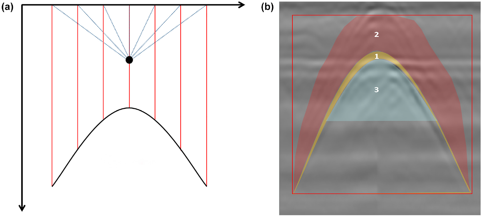
Radar wave response characteristics of targets: (a) independent target in numerical simulation; (b) a crack from the field data.

Similarly, the expertise development process in the domain of GPR entails several stages. Initially, experts acquire knowledge with respect to distinct defect characteristic spectra derived from numerical simulations, thereby establishing a preliminary understanding of the typical distress features. Subsequently, they engage in distress identification within spectra containing background noise, recognizing the inherent ambiguity that noise introduces to the distress characteristics. Finally, experts undergo training for practical detection tasks, encompassing not only background noise induced by random media but also variations in distress edge features resulting from irregular distress sizes. This training facilitates the discernment of diverse alterations in distress reflection characteristics based on typical spectra, necessitating extensive accumulative experience to achieve precise identification.

Therefore, we present a curriculum learning framework that leverages the classification of defect sample feature types to facilitate the identification of difficulty levels. Specifically, we define defect samples generated through numerical simulations in a homogeneous medium as the “simple curriculum” because of their characteristic spectra solely encompassing defect reflection features, devoid of the influence of background noise induced by random discrete road materials. Subsequently, we designate defect samples generated in a random discrete medium through numerical simulations as the “moderate-complexity curriculum,” as their characteristic spectra exhibit pronounced scattering phenomena in interlayer positions and internal structural layers, thus replicating the stochastic background noise present in actual data acquisitions, in addition to the singular defect reflection feature observed in the homogeneous medium. Lastly, we define real-world data as the “high-complexity curriculum” because its defect radar spectra encompass not only defect reflection features and background noise but also the variations in edge features resulting from the irregularities of the defects. The curriculum learning flowchart proposed in this study is depicted in Figure 2. During our training process, we adopt a three-stage approach, progressively training the convolutional neural network (CNN) model on samples that increase in difficulty. To avoid catastrophic forgetting of the model, we guarantee that each stage contains samples from the previous stage.

Figure 2.

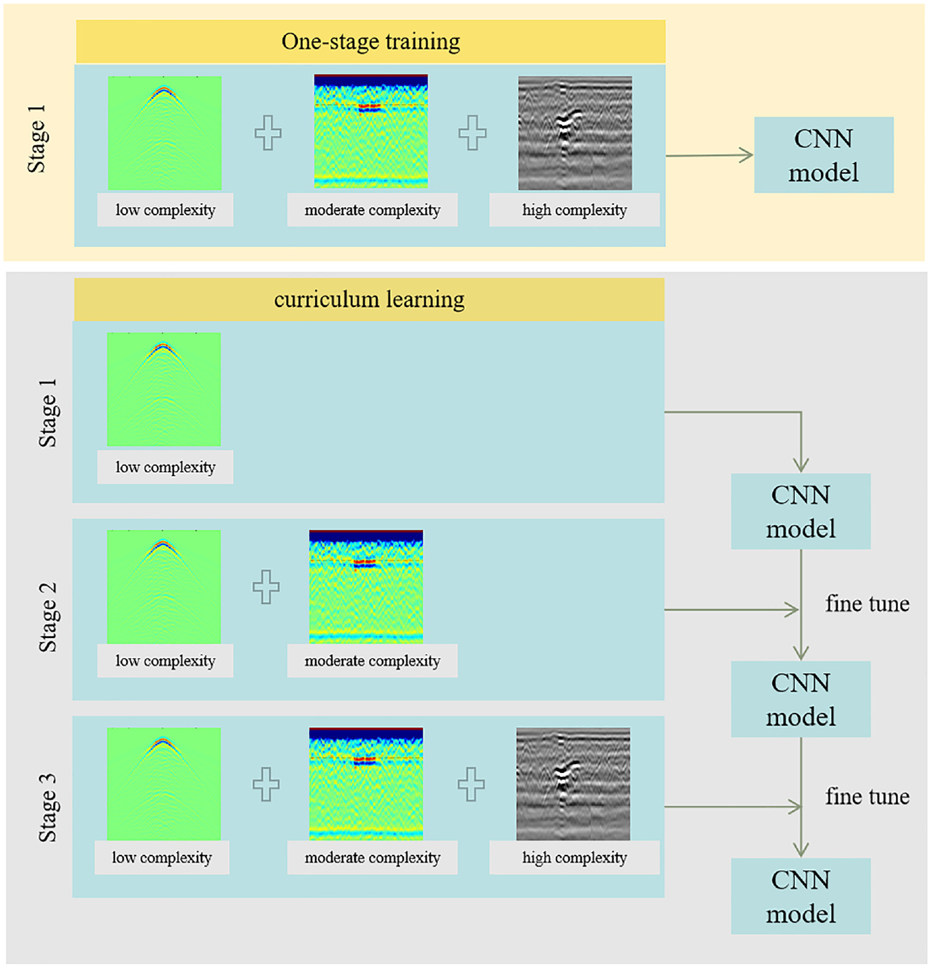
The curriculum learning flowchart: (a) stage one: low-complexity samples; (b) stage two: moderate-complexity samples + low-complexity samples; (c) stage three: high-complexity samples + moderate-complexity samples + low-complexity samples.

Data Description

Low-Complexity Samples: Simulated Distress in Homogeneous Media

To enhance the generation of diverse numerical simulation samples for distress, the study incorporates two typical road structures in the low-complexity model. Comprehensive consideration is given to the variation in dielectric parameters of materials at different locations, thereby enabling the simulation of diverse data by adjusting the dielectric parameters of individual road structure layers. The model parameters for these layers are detailed in Table 1.

Table 1.

Homogeneous Medium Model Parameters of Road Structure

Structure layer	Typical road structures 1			Typical road structures 2
Structure layer	Surface	Base layer	Soil foundation	Surface	Base layer	Soil foundation
Thickness (cm)	10	36	20	18	36	20
Dielectric constant	7–9	8–10	11–13	7–9	8–10	11–13
Conductivity	0.002	0.002	0.005	0.002	0.002	0.005

Moreover, the investigation takes into account the dynamic changes in the filling material within the distress. During the initial development stage, air occupies the internal voids, with its dielectric constant being 1. Subsequently, as the distress progress, free water enters the internal voids with a dielectric constant of approximately 78. Furthermore, the action of vehicles’ tire pumps causes continuous flushing of the internal mixture, leading to the loss of fine aggregates and the filling of the voids with a mud–water mixture. The dielectric constant of this filling material varies between that of pure water and road materials. Consequently, three substances, namely water, air, and mud–water mixture, are chosen as the filling materials for the distress.

To accurately represent the distress, numerical simulations are conducted separately for two typical cases based on the finite difference time domain method: the reflective crack and cavity, as illustrated in Figures 3 and 4. The left-hand side of each distress is the pavement structure diagram, and the colors represent the dielectric constant. The right-hand side of each distress is the simulated GPR images, and the colors represent the amplitude intensity. Notably, the uniformity of the road structure layers results in the radar waveforms within the homogeneous medium model exhibiting simplicity and cleanliness, unencumbered by random medium background noise. Consequently, these waveforms directly reflect the morphological characteristics of radar waves reaching the distress locations, thereby facilitating effective distress identification during practical detection processes. The simplicity of the representations is advantageous for human visual recognition and enables the extraction of representative distress features for deep learning convolutional networks, resulting in an impressive automatic identification accuracy of over 99%. Accordingly, datasets possessing such characteristics are categorized as “low-complexity samples.” By adjusting the dielectric constants of distinct road structure layers and the filling materials within the distress, a myriad of diverse numerical simulation samples for distress are generated, the quantities of which are tabulated in Table 2.

Figure 3.

Distress medium model and numerical simulation of typical road structures 1: (a) medium model of a crack; (b) numerical simulation of a crack; (c) medium model of a cavity; (d) numerical simulation of a cavity.

Figure 4.

Distress medium model and numerical simulation of typical road structures 2: (a) medium model of a crack; (b) numerical simulation of a crack; (c) medium model of a cavity; (d) numerical simulation of a cavity.

Table 2.

Number of Simulated Distresses

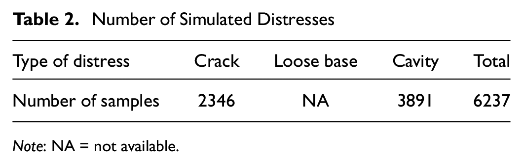
Type of distress	Crack	Loose base	Cavity	Total
Number of samples	2346	NA	3891	6237

Note: NA = not available.

Moderate-Complexity Samples: Simulated Distress in Random Discrete Media

To achieve a more realistic simulation of actual road medium models and to enhance the challenge of distress feature recognition within a homogeneous medium context, moderate-complexity samples introduce the consideration of background noise arising from a multiphase discrete random medium. By incorporating Guo et al.’s ( 3 ) proposed multiphase discrete random medium model, the simulations focus on cracks, loose base, and cavity distress, utilizing the same road structure layers as in the preceding section. In the process of generating diverse data, the manipulation of dielectric constants for individual structure layers’ materials, as well as the adjustment of the mixture’s void ratio, are employed. The detailed parameters for the multi-layer road structure are presented in Table 3.

Table 3.

Random Discrete Medium Model Parameters of Road Structure

Structure layer	Thickness (cm)	Aggregate (A)/soil		Binding material (B)		Volume of air voids (%)	Volume ratio of B to A (%)
Structure layer	Thickness (cm)	Dielectric constant	Conductivity	Dielectric constant	Conductivity	Volume of air voids (%)	Volume ratio of B to A (%)
Surface	10/18	7–9	0.001	4–5	0.003	3–5	35
Base layer	36	7–9	0.001	8–9	0.003	3–5	35
Soil foundation	20	11–13	0.005	NA	NA	1	NA

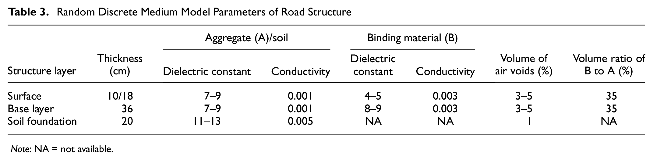
Note: NA = not available.

Numerical simulations are conducted for three representative distress types: cracks, loose base, and cavity distress, as visualized in Figures 5 and 6. The introduced multiphase discrete medium model exhibits significant scattering phenomena at both interlayer positions and within the structure layers, yielding radar waveforms characterized by stochastic background noise that closely approximates actual collected data. Consequently, the reflection characteristics of the three distress types are influenced by this random background noise, engendering a certain level of complexity in identifying their morphological features. As a result, such distresses are classified as exhibiting a moderate level of identification difficulty, encompassing both the direct reflection features of the distress and the distinct characteristics of random background noise. Through deliberate adjustments to the dielectric constants of various road structure layers and the void ratio of the mixture, a diverse set of numerical simulation samples for distress is generated, with the specific quantities of simulated samples provided in Table 4.

Figure 5.

Distress medium model and numerical simulation of typical road structures 1: (a) medium model of a crack; (b) numerical simulation of a loose base; (c) medium model of a cavity; (d) numerical simulation of a loose base; © medium model of a cavity; (f) numerical simulation of a cavity.

Figure 6.

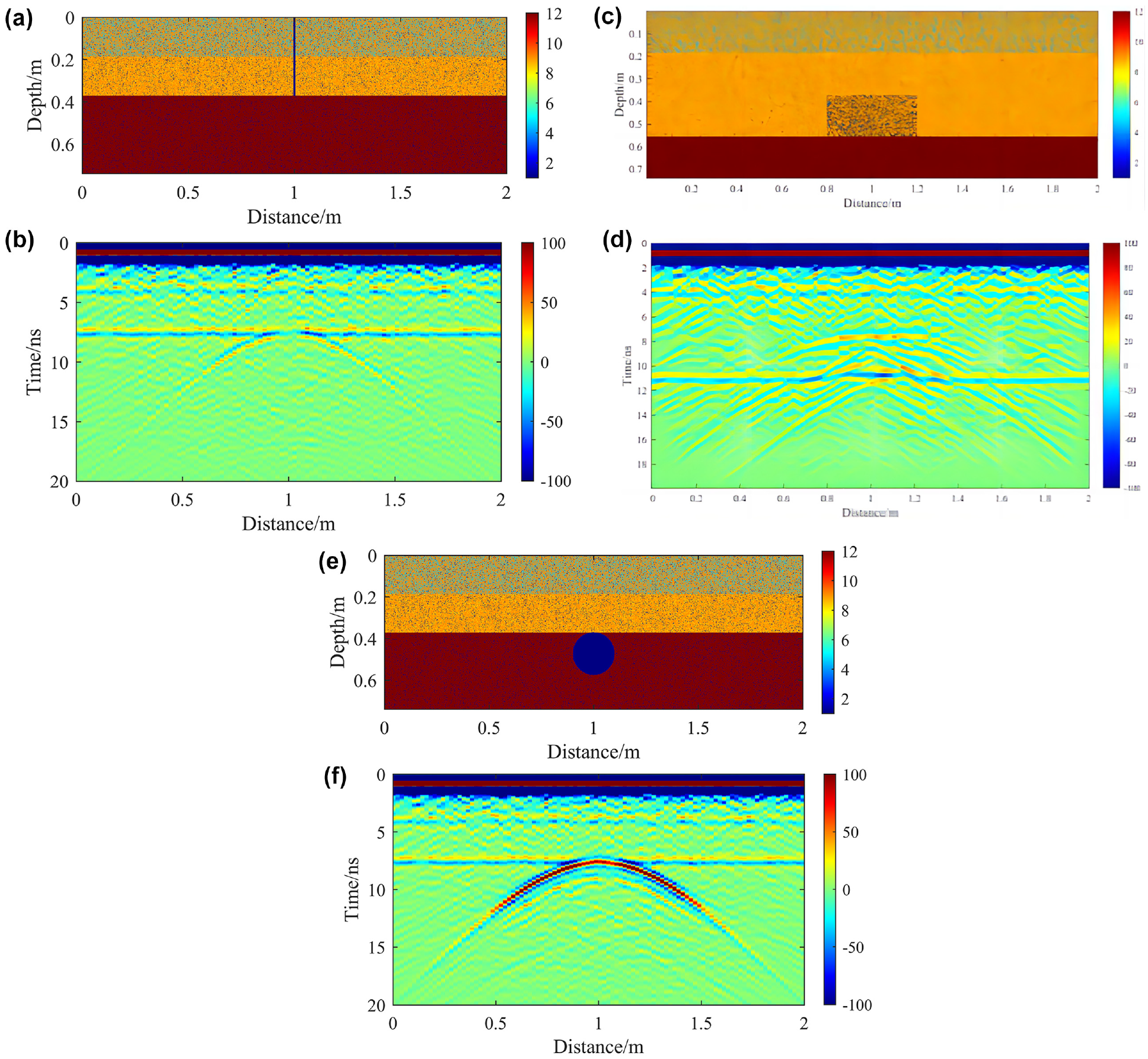
Distress medium model and numerical simulation of typical road structures 2: (a) medium model of a crack; (b) numerical simulation of a loose base; (c) medium model of a cavity; (d) numerical simulation of a loose base; (e) medium model of a cavity; (f) numerical simulation of a cavity.

Table 4.

Number of Simulated Distresses

Type of distress	Crack	Loose base	Cavity	Total
Number of samples	1665	1154	2528	5347

High-Complexity Samples: Distress from the Field Data

During the investigation of RSD in the field using GPR, various challenges arise from both the influence of random discrete medium background noise present in the road environment and the irregular morphological characteristics of the distresses themselves. The irregular edges of the distress affect the radar wave reflection features, adding complexity to their identification. While numerical simulations based on a random discrete medium have provided a closer approximation of actual distress reflection characteristics, they are limited by the constraints of finite difference numerical simulation methods, making it difficult to precisely model distress with irregular morphologies. The presence of irregular volume characteristics in distress further leads to random EW scattering, causing the superposition of disordered scattered waves and distress-reflected waves, resulting in a noticeable decrease in the resolution of distress echoes. To address these challenges, real distress data collected in the field is used, and it is classified as high-complexity samples because of the increased complexities associated with their identification. A four-channel GPR system was used for the detection of RSD because it can be mounted on a vehicle with fast speed and high coverage area. Then the hand-towed GPR device was used for detailed detection at the location of distresses. Most of the GPR data for training in this paper was collected by hand-towing the GPR device to ensure the data’s quality. The GPR system mentioned above is the ground-coupled data acquisition that shown in Figure 7. Figure 7a shows the four-channel GPR system with one 200 MHz antenna, two 400 MHz antennas, and one 900 MHz antenna. Figure 7b shows the four-channel GPR system mounted on a vehicle.

Figure 7.

The ground penetrating radar (GPR) system: (a) the four-channel GPR system; (b) the GPR system was mounted on a vehicle (Guanghua Yue took the photos).

To ensure the diversity of data, we selected urban roads and highways for data collection. Twenty-three road sections from five urban roads and six highways in China were detected, with a total length of 2408 km. The five urban roads are located in Xi’an, Zhengzhou, Kaifeng, Shanghai, and Huainan, and the six highways are located in Anhui, Shaanxi, Henan, and Zhejiang, which cover the northern and southern cities in China. The collected GPR image and verified distress are shown in Figures 8 –10. Figure 8a shows the GPR image of the crack, Figure 8b shows that the crack was verified by coring, and Figure 8c shows the core drilling machine in crack distress. Figure 9a shows a GPR image of the loose base, Figure 9b shows that the loose base was verified by digging pits, and Figure 9c shows a field picture at loose base distress location. Figure 10a shows the GPR image of the cavity, Figure 10b shows the cavity was verified by an industrial endoscope though a 2 cm diameter borehole, and Figure 10c shows the industrial endoscope.

Figure 8.

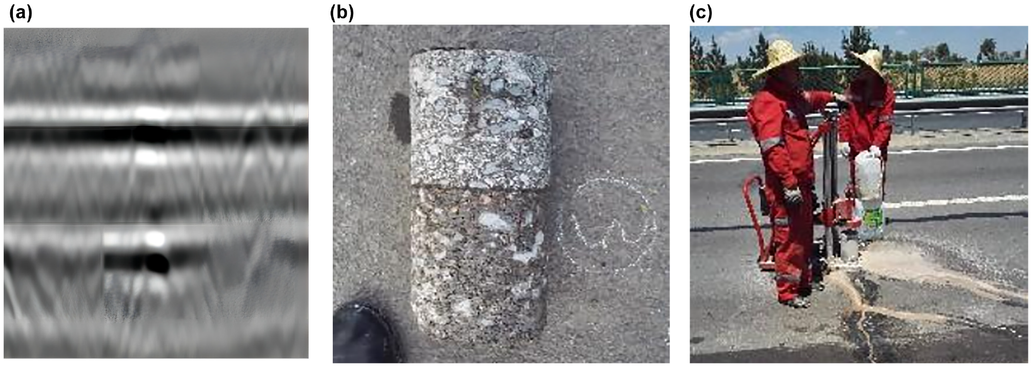
The collected ground penetrating radar (GPR) images of the crack and verified distress: (a) GPR image of the crack; (b) the crack was verified by coring; (c) the core drilling machine.

Figure 9.

The collected ground penetrating radar (GPR) images of the loose base and verified distress: (a) GPR image of the loose base; (b) loose base was verified by digging pits; (c) field picture at the loose base distress location.

Figure 10.

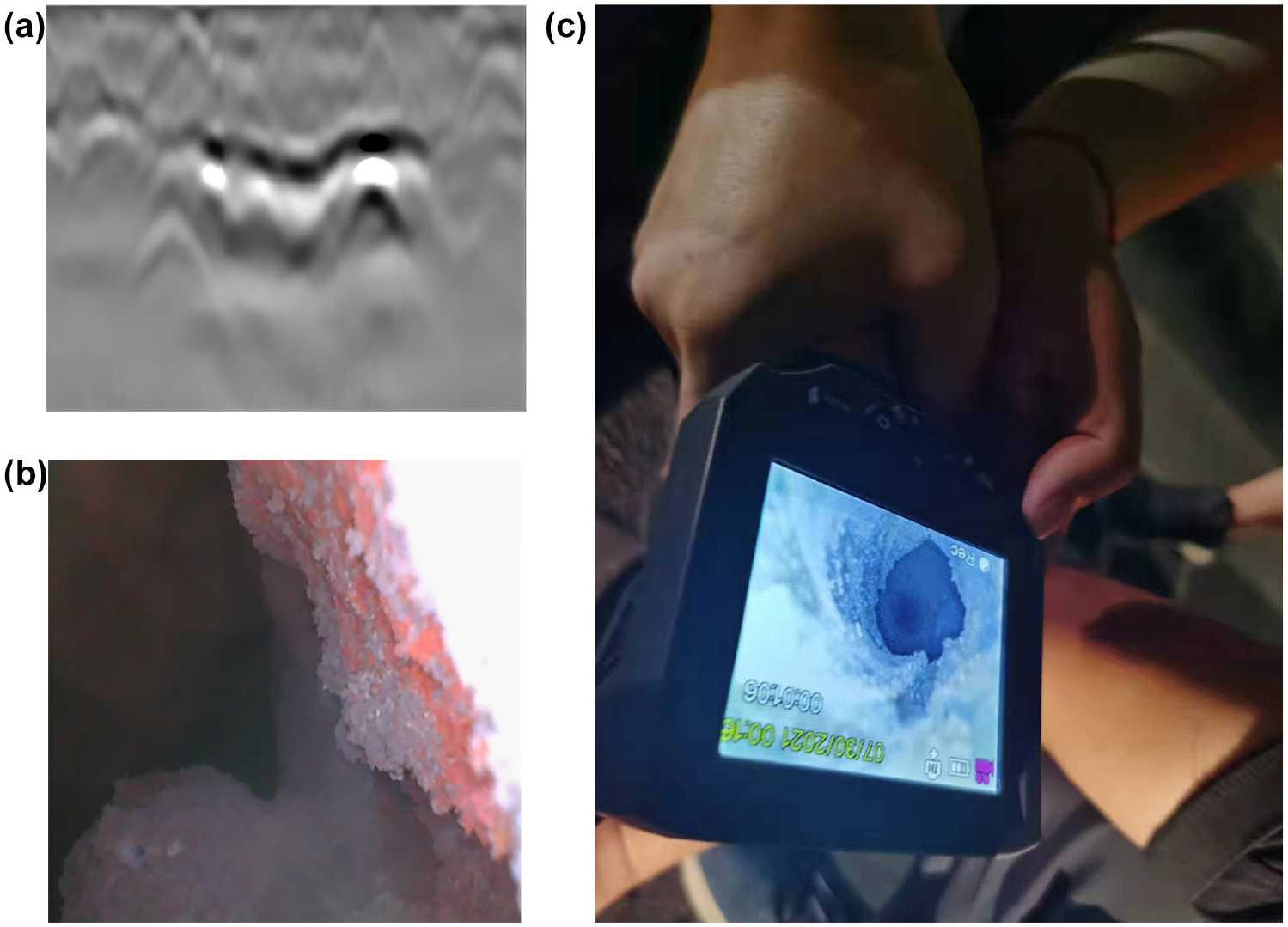
The collected ground penetrating radar (GPR) images of the cavity and verified distress: (a) GPR image of the cavity; (b) the cavity was verified by an industrial endoscope; (c) the industrial endoscope.

Three representative distress types: a crack, loose base, and cavity distress, are collected, and parts of the samples are visualized in Figures 11 –13. The quantity of samples utilized in the analysis is detailed in Table 5.

Figure 11.

Partial samples of crack distress from field data: (a)–(e) GPR images of the crack.

Figure 12.

Partial samples of loose base distress from field data: (a)–(e) GPR images of the loose base.

Figure 13.

Partial samples of cavity distress from field data: (a)–(e) GPR images of the cavity.

Table 5.

Number of Samples from Field Data

Type of distress	Crack	Loose base	Cavity	Total
Number of samples	2448	1832	3148	7428

Sample Statistics

In the context of developing a multi-source dataset, the dataset encompasses 6237 samples representing low-complexity instances, 5347 samples reflecting moderate complexity, and a substantial collection of 7428 samples characterized by high complexity. Subsequently, a random partitioning procedure is applied to the high-complexity samples, where 70% of the samples are allocated to the training set, and the remaining 30% constitute the test set. Moreover, the samples drawn from the simple- and moderate-complexity instances are combined to form the training dataset. The specific distribution of these samples is elaborated in Table 6.

Table 6.

Distribution of Training and Testing Samples

Type of samples	Low complexity	Moderate complexity	High complexity	Total
Training set	6237	5347	5200	16,784
Testing set	NA	NA	2228	2228

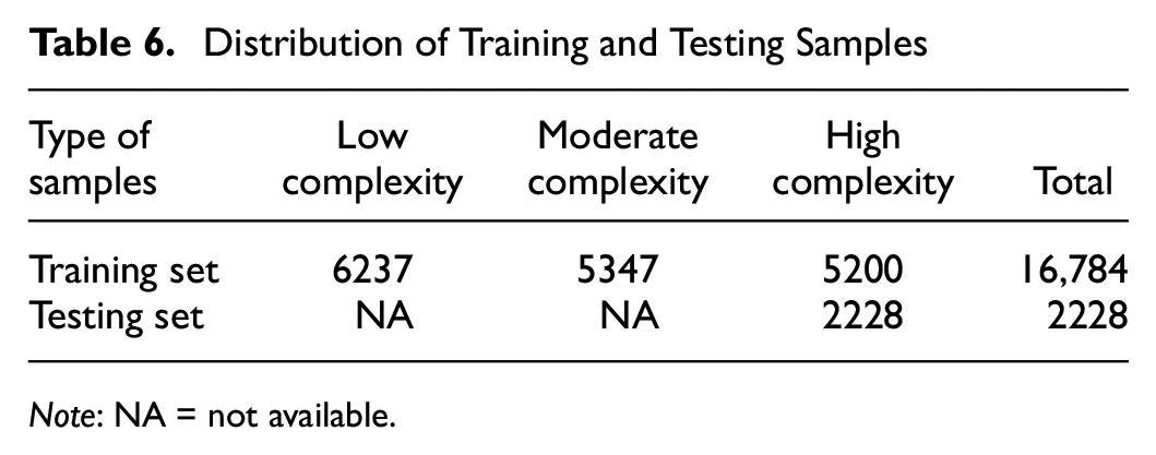
Note: NA = not available.

Case Study

Deep Learning Model Parameter Setting

With respect to the curriculum learning mentioned earlier, we conducted experiments using the two most commonly employed models in the field of GPR target recognition: the Faster R-CNN (region-based convolutional neural network) and You Only Look Once version 7 (YOLOv7). The training parameters for these models are presented in Table 7. Each training stage is set to consist of 100 epochs, resulting in a total of 300 epochs over three stages. For all three difficulty samples, a unified single-stage training approach is employed, with the training epochs directly set to 300. Model performance is evaluated using metrics such as precision (P), recall (R), $F_{1}_score$ , and mean average precision (mAP). The evaluation metrics can be calculated as follows:

Table 7.

The Training Parameters for These Models

Model parameters	Batch size	Image size	Momentum	Decay	Learning rate	Epochs
Value	32	416*416	0.937	0.0005	0.001	300

P = \frac{TP}{TP + FP}

(6)

R = \frac{TP}{TP + FN}

(7)

In Equations 6 and 7, $TP$ is the number of true positives, $FP$ is the number of false positives, $FN$ is the number of false negatives, $P$ denotes how well the model performed in classifying an object positive, and $R$ denotes the ability to detect the positive samples:

F_{1}_score = 2 \cdot \frac{P \cdot R}{P + R}

(8)

AP = \int_{0}^{1} P (r) \cdot dr

(9)

The values of $F_{1}_score$ combine the result of $P$ and $R$ that range from [0, 1], in which 1 denotes the best output of the model and 0 denotes the worst output of the model. Here, $AP$ is defined as the area under the $P - R$ curve, which measures the accuracy of the model for each class, and $mAP$ is the average of $AP$ for all classes.

Model Performance Comparison

To conduct a comprehensive comparative analysis of the proposed curriculum learning training process in this research, two additional training methodologies are concurrently considered. The first approach involves training the model directly on a diverse mixture of samples encompassing three distinct types. The second approach adopts an anti-curriculum learning strategy, wherein the training process is altered from the curriculum learning-based paradigm. Specifically, the model is initially trained on high-complexity samples, followed by training on moderate-complexity samples, with the primary objective of validating the observed performance improvements, substantiating that they indeed stem from the differential sample selection at each training stage. Subsequently, the weights obtained at the culmination of the training process are utilized to assess the model’s performance on the testing set. The computed results pertaining to the model performance metrics are meticulously documented and are presented in Table 8 for thorough analysis and discussion.

Table 8.

Model Performance Calculation Results in the Testing Set

Training strategy	Precision	Recall	F1_score	mAP
YOLOv7
Only high-complexity samples	0.751	0.669	0.708	0.746
Single-stage training: high-complexity samples + moderate-complexity samples + low-complexity samples	0.784	0.713	0.747	0.753
Curriculum learning: low-complexity samples then (low complexity + moderate complexity) then (low complexity + moderate complexity + high complexity)	0.842	0.789	0.815	0.799
Anti-curriculum learning: high-complexity samples then (high complexity + moderate complexity) then (high complexity + moderate complexity + low complexity)	0.782	0.709	0.744	0.752
Faster R-CNN
Only high-complexity samples	0.756	0.678	0.721	0.748
Single-stage training: high-complexity samples + moderate-complexity samples + low-complexity samples	0.791	0.718	0.753	0.762
Curriculum learning: low-complexity samples then (low complexity + moderate complexity) then (low complexity + moderate complexity + high complexity)	0.854	0.801	0.827	0.811
Anti-curriculum learning: high-complexity samples then (high complexity + moderate complexity) then (high complexity + moderate complexity + low complexity)	0.788	0.716	0.750	0.748

Note: mAP = mean average precision; YOLOv7 = You Only Look Once version 7; R-CNN = region-based convolutional neural network.

The results depicted in Table 8 manifest that the YOLOv7 model, when subjected to three distinct training strategies, demonstrated optimal performance when following the proposed curriculum learning-based training strategy, the best model results are shown in bold entries. In comparison to direct training on the inadequately gathered field data (high-complexity samples), the curriculum learning-based training exhibited noteworthy enhancements in precision by 12.1%, recall by 17.9%, F1_score by 15.1%, and mAP by 7.1%. Similarly, when compared to training on the mixed sample datasets directly, the curriculum learning-based training led to improvements in precision by 7.4%, recall by 10.7%, F1_score by 9.1%, and mAP by 6.1%. Conversely, the adoption of anti-curriculum learning did not yield models that outperformed those trained on mixed samples, indicating that the efficacy of the curriculum learning-based training strategy primarily lies in the sample selection across different stages rather than being influenced by individual training phases.

During training with the Faster R-CNN model, noteworthy improvements were observed in precision by 13.0%, recall by 18.1%, F1_score by 14.7%, and mAP by 8.4% when directly compared to models trained on the high-complexity samples. Similarly, compared to training on the mixed sample datasets directly, the Faster R-CNN model showed improvements in precision by 8.0%, recall by 11.6%, F1_score by 9.8%, and mAP by 6.4%. Despite achieving better performance than the YOLOv7 model, the Faster R-CNN model incurred a significant decline in processing speed. While the YOLOv7 model achieved a recognition speed of 56 frames per second (FPS), the Faster R-CNN model’s recognition speed was notably lower, reaching only 8 FPS, resulting in a speed decrease of over 85%.

Conclusions

Numerical simulation and data augmentation techniques are important means to address the issue of insufficient GPR samples. However, if the field samples and simulated samples are randomly input into the model for training, disregarding sample complexity differences and the model’s learning status may lead to suboptimal local minima rather than achieving a globally optimal solution. To mitigate this limitation, we proposed a novel approach by delving into the training strategy of the network model and analyzing the distinctive characteristics of GPR distress interpretation. Inspired by simulating expert training procedures, we used curriculum learning to simulate the training process of experts, allowing the model training to progress from low complexity to difficult. This strategy is subsequently employed to evaluate the suitability and performance of two widely used object detection models, namely YOLOv7 and the Faster R-CNN, under the proposed framework. Experimental results reveal that compared to conventional mixed sample training, the model’s precision demonstrates respective improvements of 7.4% and 8.0%, recall exhibits respective enhancements of 10.7% and 11.6%, F1_score indicates respective gains of 9.1% and 9.8%, and mAP displays respective increments of 6.1% and 6.4%.

It should be noted that the curriculum learning framework proposed here incorporates difficulty evaluators and training schedulers determined through expert prior knowledge, independent of data-driven algorithms. Consequently, the framework may possess a certain degree of subjectivity. To address this concern and advance the research, future investigations ought to explore the application of data-driven models or algorithms to determine difficulty evaluators and training schedulers, thereby reducing the impact of human-driven design elements.

Footnotes

Author Contributions

The authors confirm contribution to the paper as follows: study conception and design: G. Yue, C. Liu; data collection: Q. Gao, Y. Du; analysis and interpretation of results: C. Liu, Y. Li; draft manuscript preparation: G. Yue. All authors reviewed the results and approved the final version of the manuscript.

Declaration of Conflicting Interests

The author(s) declared no potential conflicts of interest with respect to the research, authorship, and/or publication of this article.

Funding

The author(s) disclosed receipt of the following financial support for the research, authorship, and/or publication of this article: This study was supported by the National Natural Science Foundation of China (52108411), the Scientific Research Project of Shanghai Science and Technology Commission (23QB1404900), the Belt and Road Cooperation Program under the 2023 Shanghai Action Plan for Science, Technology and Innovation (No. 23210750500), the Fundamental Research Funds for the Central Universities (22120230311), and the Scientific Research Project of Shanghai Municipal Commission of Housing and Urban-rural Development (2021-002-032).

ORCID iDs

Guanghua Yue

Chenglong Liu

Yishun Li

Yuchuan Du

The authors are responsible for all views and opinions expressed in this paper.

References

Liu

Nie

Cao

F. A.

Response-Type Road Anomaly Detection and Evaluation Method for Steady Driving of Automated Vehicles. IEEE Transactions on Intelligent Transportation Systems, Vol. 23, 2022, pp. 21984–21995.

Yue

Liu

Guo

GPR Data Augmentation Methods by Incorporating Domain Knowledge. Applied Sciences, Vol. 12, 2022, p. 10896.

Guo

Zhu

Detection and Characterization of Cracks in Highway Pavement With the Amplitude Variation of GPR Diffracted Waves: Insights from Forward Modeling and Field Data. Remote Sensing, Vol. 14, 2022, p. 976.

Liu

Yue

Gao

Deep Learning-Based Pavement Subsurface Distress Detection via Ground Penetrating Radar Data. Automation in Construction, Vol. 142, 2022, p. 104516.

Yuan

Liu

Cai

Integrated Processing of Image and GPR Data for Automated Pothole Detection. Journal of Computing in Civil Engineering, Vol. 30, 2016, p. 04016015.

Gao

Yuan

Tong

Yang

Autonomous Pavement Distress Detection Using Ground Penetrating Radar and Region-Based Deep Learning. Measurement, Vol. 164, 2020, p. 108077.

Dong

Gao

Fang

Zhang

Xue

Zhang

Rapid Detection Methods for Asphalt Pavement Thicknesses and Defects by a Vehicle-Mounted Ground Penetrating Radar (GPR) System. Sensors, Vol.16, 2016, p. 2067.

Lei

Hou

Tan

Jiang

Liu

Automatic Hyperbola Detection and Fitting in GPR B-Scan Image. Automation in Construction, Vol. 106, 2019, p. 102839.

Harkat

Dosse Bennani

Ground Penetrating Radar Imaging for Buried Cavities in a Dispersive Medium: Profile Reconstruction Using a Modified Hough Transform Approach and a Time-Frequency Analysis. International Journal on Communications Antenna and Propagation (IRECAP), Vol. 5, 2015, pp. 78–92.

10.

Frigui

Gader

Detection and Discrimination of Land Mines in Ground-Penetrating Radar Based on Edge Histogram Descriptors and a Possibilistic $K$-Nearest Neighbor Classifier. IEEE Transactions on Fuzzy Systems, Vol. 17, 2009, pp. 185–199.

11.

Liu

Jiang

Wang

Enabling Edge Computing Ability in View-Independent Vehicle Model Recognition. International Journal of Transportation Science and Technology, 2023, pp. 1–14.

12.

Liu

Weng

Cao

Effective Pavement Skid Resistance Measurement Using Multi-Scale Textures and Deep Fusion Network. Computer-Aided Civil and Infrastructure Engineering, Vol. 38, 2023, pp. 1041–1058.

13.

Puntu

J. M.

Chang

Lin

Amania

H. H.

Doyoro

Y. G.

A Comprehensive Evaluation for the Tunnel Conditions With Ground Penetrating Radar Measurements. Remote Sensing, Vol.13, 2021, pp. 4250.

14.

Todkar

S. S.

Le Bastard

Baltazart

Ihamouten

Dérobert

Performance Assessment of SVM-Based Classification Techniques for the Detection of Artificial Debondings Within Pavement Structures from Stepped-Frequency A-Scan Radar Data. NDT & E International, Vol. 107, 2019, p. 102128.

15.

Zhang

Zheng

Dong

Tian

Jia

In-Situ Recognition of Moisture Damage in Bridge Deck Asphalt Pavement With Time-Frequency Features of GPR Signal. Construction and Building Materials, Vol. 244, 2020, p. 118295.

16.

Ali

Zaidi

A. F. A.

Meng

C. E.

Ahmad

M. R.

Amran

T. S. T.

Kanafiah

S. N. A. M.

Fook

C. Y.

Shukor

S. A. A.

Elshaikh

Shape Classification of Ground Penetrating Radar Using Discrete Wavelet Transform and Principle Component Analysis. IOP Conference Series: Materials Science and Engineering, Vol. 705, 2019, p. 12046.

17.

Klęsk

Godziuk

Kapruziak

Olech

Fast Analysis of C-Scans From Ground Penetrating Radar via 3-D Haar-Like Features With Application to Landmine Detection. IEEE Transactions on Geoscience and Remote Sensing, Vol. 53, 2015, pp. 3996–4009.

18.

Schmidhuber

Deep Learning in Neural Networks: An Overview. Neural Networks, Vol. 61, 2015, pp 85–117.

19.

Che

Liu

Cross-Scene Pavement Distress Detection by a Novel Transfer Learning Framework. Computer-Aided Civil and Infrastructure Engineering, Vol. 36, 2021, pp. 1398–1415.

20.

Zhang

Sun

Recognition of the Typical Distress in Concrete Pavement Based on GPR and 1D-CNN. Remote Sensing, Vol. 13, 2021, p. 2375.

21.

Liu

Zou

Dong

Wang

GPR-Based Detection of Internal Cracks in Asphalt Pavement: A Combination Method of DeepAugment Data and Object Detection. Measurement, Vol. 197, 2022, p. 111281.

22.

Qin

Zhang

Tang

Wang

Automatic Recognition of Tunnel Lining Elements from GPR Images Using Deep Convolutional Networks With Data Augmentation. Automation in Construction, Vol. 130, 2021, p. 103830.

23.

Luo

Lei

Hou

Wang

Ren

Zhang

Luo

Wang

GPR B-Scan Image Denoising via Multi-Scale Convolutional Autoencoder With Data Augmentation. Electronics, Vol. 10, 2021, p. 1269.

24.

Pham

Lefèvre

Buried Object Detection from B-Scan Ground Penetrating Radar Data Using Faster-RCNN. IGARSS 2018 - 2018 IEEE International Geoscience and Remote Sensing Symposium, Valencia, Spain, 2018, pp. 6804–6807.

25.

Reichman

Collins

L. M.

Bralich

Improving Convolutional Neural Networks for Buried Target Detection in Ground Penetrating Radar Using Transfer Learning via Pretraining. Detection and Sensing of Mines, Explosive Objects, and Obscured Targets XXII. International Society for Optics and Photonics. Proceedings of the SPIE, Vol. 10182, No. 101820X, 2017.

26.

Kang

Kim

Lee

J. J.

Deep Learning-Based Automated Underground Cavity Detection Using Three-Dimensional Ground Penetrating Radar. Structural Health Monitoring, Vol. 19, 2020, 173–185.

27.

Conyers

L B.

Leckebusch

Geophysical Archaeology Research Agendas for the Future: Some Ground-Penetrating Radar Examples. Archaeological Prospection, Vol. 17, No. 2, 2010, pp. 117–123.

28.

Ozkaya

Ozturk

Melgani

Seyfi

Residual CNN Plus Bi-LSTM Model to Analyze GPR B Scan Images. Automation in Construction, Vol. 123, 2021, p. 103525.

29.

Wang

Ouyang

Liu

Liao

Zhou

Buried Target Detection Method for Ground Penetrating Radar Based on Deep Learning. Journal of Applied Remote Sensing, Vol. 16, 2022, p. 18503.

30.

Hou

Lei

Deep Learning-Based Subsurface Target Detection From GPR Scans. IEEE Sensors Journal, Vol. 21, 2021, pp. 8161–8171.

31.

Liu

Large-Scale Pavement Roughness Measurements With Vehicle Crowdsourced Data Using Semi-Supervised Learning. Transportation Research Part C: Emerging Technologies, Vol. 125, 2021, p. 103048.

32.

Weng

Ablat

Liu

A Novel Approach for Pavement Texture Characterisation Using 2D-Wavelet Decomposition. The International Journal of Pavement Engineering, Vol. 23, 2022, pp. 1851–1866.

33.

Shorten

Khoshgoftaar

T. M.

A Survey on Image Data Augmentation for Deep Learning. Journal of Big Data, Vol. 6, 2019, pp. 1–48.

34.

Bengio

Louradour

Collobert

Weston

Curriculum learning. Proc., 26th Annual International Conference on Machine Learning, 2009, pp. 41–48.

35.

Wang

Chen

Y. D.

Zhu

W. W.

A Survey on Curriculum Learning. IEEE Transactions on Pattern Analysis and Machine Intelligence, Vol. 44, 2022, pp. 4555–4576.