The use of probabilistic analysis (PA) of slopes as an effective method for evaluating the uncertainty that is so pervasive in variables has become increasingly common in recent years. This study presents a case study which was conducted to demonstrate the efficiency of an embankment which consists of an 11.693 m-high soil slope, placing emphasis on PA and reliability evaluation. The investigation employs Monte Carlo simulation (MCS) and subset simulation (SS) techniques, considering seismic coefficients (kh) of 0.12 for Zone-III and 0.14 for Zone-IV, along with varying pore water pressure ratios (ru=0.0, , and ). MCS with 10,000 samples was used to test the probabilistic response of the proposed embankment. This work also discusses the results of SS, in which 1,400 samples are generated from UPSS 3.0 Excel add-ins, which permits rapid PA in such a way that they progressively shift toward the failure zone in successive stages. The study delves into the impact of uncertainty on the probability of failure . Findings reveal an increased with rising coefficients of variation, , and kh values, underscoring the sensitivity to soil parameter variations. SS outperforms MCS in simulating low probabilities, demanding smaller sample sizes and less computational time. Furthermore, the machine learning technique has been used to optimize the worst condition. In this current research, three neural network-based models, namely recurrent neural network, long short-term memory (LSTM), and Bayesian neural network, have been used. Based on the performance of the models, the three neural network-based models were compared in the testing phase, and the proposed LSTM outperformed the other neural networks (R2 = 0.9962 and root mean square error = 0.0051).
Geotechnical structures, including slopes and soil embankments, can be naturally occurring, artificially cut, or manufactured. These structures are often found near or integrated into larger engineered structures like highways, railways, bridges, and dams (1, 2). However, the instability of slopes can pose a considerable risk to human safety, leading to property damage, financial losses, and even fatalities (3). Therefore, evaluating the stability of both natural and engineered slopes is crucial for effective risk management and the prevention of failures (4). The primary purpose of analyzing slope stability is to evaluate the slope’s capacity to withstand failure caused by sliding along a potential slip surface, whether it is a natural slope or an engineered one. In addition, the slope stability analysis is aimed at assessing the safety of the slope in relation to the possibility of sliding. The factor of safety (FS) is an index of the level of security provided by the relationship between the forces or moments that resist failure and those that potentially drive failure. It is typically calculated using traditional deterministic approaches such as the limit equilibrium method (LEM), the strength reduction method (SRM), the limit analysis method, the finite element method (FEM), or the finite difference method. However, LEM and SRM are the most frequently employed methods among researchers and practitioners (5, 6). When assessing the stability of a slope, a FS of less than 1 is conventionally considered an indication of instability. However, the characteristics of the soil and rock that make up a slope can vary significantly depending on various factors. For example, the type of rock that the soil originated from, weathering, erosion, and sedimentation conditions can all influence the properties of the soil at different depths. This is commonly known as the inherent spatial variability of the soil (7, 8). When addressing the inherent spatial variability of slopes, one of the most important effects is the variation in the critical slip surface, which is the surface along which the slope is most likely to fail. The location and shape of the critical slip surface can vary as a result of the variability in the geotechnical properties of the slope, which can lead to variations in the minimum FS (9). Understanding and accounting for these variations is crucial in ensuring the safe and sustainable design of slopes. In the process of analyzing the stability of a slope, one of the most fundamental steps is to locate the critical slip surface among the many probable slip surfaces. The slope can be analyzed as a series system, with the critical slip surface representing the weakest one (10–12). In addition, geotechnical structure design and analysis are also affected by measurement uncertainty, statistical uncertainty, and transformation model uncertainty. These geotechnical uncertainties are not capable of being taken into account by conventional deterministic analytical methods. First of all, there are many different causes of uncertainty, including variations in soil characteristics, building techniques, and environmental factors (13). Omitting uncertainty may result in unduly optimistic or pessimistic assessments of the slope’s stability and safety, which may lead to insufficient design features or needless expenses and unexpected failures. To further emphasize the importance of uncertainty we refer the reader to the published articles by Yin (14) and Jia et al. (15).
As a result, probabilistic stability methodologies are becoming more common in geotechnical engineering, as they provide a means of explicitly incorporating the underlying uncertainties in soil and rock properties. These methodologies offer an effective tool for quantifying the safety factor of geotechnical structures by assessing failure probability or reliability index (β). Therefore, these concepts have gained popularity in geotechnical engineering, and their use is becoming increasingly widespread (16–23).
In recent decades, numerous researchers have made significant contributions to the study of the probabilistic slope stability of embankments (20, 24–29). Malkawi et al. commenced a reliability analysis (RA) of slopes using two different approaches: the first-order second moment method (FOSM) and the Monte Carlo simulation (MCS) technique (30). The analysis was based on four well known deterministic methods: ordinary method of slices (OMS), Bishop simplified method (BSM), simplified Janbu method and Spencer method. Griffiths et al. used random FEM to study slope stability considering spatial variability in soil strength parameters (31). Huang et al. employed random FEM (RFEM) in their investigation of slope system reliability and highlighted that RFEM presents a complete way of evaluating the slope system RA (32). Ray and Baidya analyzed the β of a slope stability problem using three different methods: mean FOSM, point estimate method, and MCS (33). The researchers considered three random variables: unit weight , angle of internal friction , and cohesion (c) in their analysis. Their findings indicated that the uncertainty in had a greater impact on the β than the uncertainties in c or . Wang et al. proposed an advanced version of MCS called a subset simulation (SS)-based approach for estimating β in a slope stability problem (9). The authors performed a comparative analysis of various reliability techniques, such as the FOSM, first-order reliability method (FORM), and MCS methods, using the commercial slope stability software (SLOPE/W). Furthermore, they also compared the SS-based probability of failure , implemented through an Excel package with the other methods. Johari and Javadi employed the jointly distributed random variables (JDRV) approach to perform a probabilistic analysis (PA) and assess the RA of an infinite slope (34). The author selected the uncertain soil parameters (i.e., c, and ) which they modeled using truncated normal probability distribution functions. The results of their analysis showed that the JDRV method is an appropriate technique for evaluating the β of an infinite slope. Li et al. created a system reliability strategy that incorporates MCS and realistic slip surfaces to assess the likelihood (12). Cho made use of multi-point FORM approach, which provided the likelihood of the union of approximation occurrences, to calculate the slope (35). Zhang et al. provide valuable insights into the application of MCS for analyzing system failure probability in the context of slope stability problems (36). The approach presented in their research can be used to effectively evaluate the system while reducing computational costs. Jiang et al. developed a method for efficiently estimating in a spatial variable soil using MCS and LEM techniques (37). The approach uses representative slip surfaces and multiple stochastic response surfaces to facilitate slope system RA. According to the findings, the proposed method was able to provide precise estimations of the and also demonstrated a considerable improvement in computational efficiency, particularly for a small level of probability. Li et al. used an SS-based random FEM approach to incorporate small probability level (i.e., ) for RA and risk (38). Furthermore, comparative analysis was done between SS-based random FEM and MCS-based random FEM. Based on the results obtained, authors found that the proposed SS-based random FEM has greatly reducing computational time compared with the MCS-based random FEM at small probability. Luo et al. investigate the PA of simple geosynthetic reinforced soil slopes using SRM in combination with FEM (39). Based on the experiment, the authors concluded that can be greatly reduced by adding a geosynthetic reinforcement layer to the constructed slope. Van Den Eijnden and Hicks’ investigation of slope stability analysis using SRM and PA has been done using modified version of SS (40). Additionally, comparative analysis was conducted between SS-based SRM and MCS-based SRM. The results showed that SS-based SRM achieved better computational efficiency and a failure probability of less than compared with MCS. Hicks and Li examined the RA of an embankment with varying slope length, and they also analyzed the impact of soil spatial variability on very long embankments (26). Ji et al. studied RA of spatial variability soil slopes using the Hasofer–Lind–Rackwitz–Fiessler algorithm for FORM (41). Johari and Mousavi employed the JDRV method to conduct the RA of soil slopes and evaluated the performance of four different LEMs, namely BSM, Janbu method, Morgenstern–Price method, and Spencer’s method (42). In addition, they compared the JDRV method with the MCS method and observed that the former requires considerably less time to assess the efficiency of the proposed approach. Guo et al. analyzed the PA of an embankment by considering spatial variability of soil (43). They utilized Karhunen–Loève Expansion to model effective c and with cross-correlated lognormal random fields. Furthermore, PA was conducted using a meta-modeling technique that combines sparse polynomial chaos expansion with global sensitivity analysis. Jiang et al. used Hermite polynomial chaos expansion to develop a non-intrusive technique for PA of an unsaturated embankment slope (28). Mahmoudi et al. utilized a mesh adaptivity and SS approach to improve the efficiency of machine learning (ML)-based reliability evaluations (44). The authors demonstrated that SS can decrease the computational time by a maximum of 60%, and they also established that fine mesh convergence for FS values is achievable. Moreover, they found that mesh adaptivity can reduce the computational time as much as 83% in comparison with utilizing fine mesh. Song et al. (45) introduced a novel method for 3D slope RA using the radial basis function network (RBFN) intelligent response surface method. Furthermore, the RBFN intelligent response surface method compared its outcomes with the MCS technique. The findings of the comparison exhibited a high degree of similarity between the two methods, indicating that the RBFN approach is a promising alternative to MCS for 3D slope RA. Deng et al. (21) employed another technique for RA of spatial variability of soil slope in their study. Specifically, they used sliced inverse regression-based multivariate adaptive regression spline approach. Ma et al. proposed reliability-based ML and advance FOSM approach for a slope stability analysis (46). In this investigation, authors predicted FS using a multi-kernel relevance vector and then FOSM approach for estimating β. Hu et al. applied a Kriging-based active learning method to improve the RA of a slope (47). Additionally, the authors also used the water-based optimization algorithm for turbulent flow to estimate the correlation parameter of the Kriging approach. This enhanced approach proved to be efficient in providing precise estimates for a complex slope problem comprising multiple layers, with a remarkable computational time of only 0.19 h. Zeng et al. introduced a classification-based surrogate model to enhance the RA and classification of a layered soil slope (48). The authors employed a binary classification approach and support vector machine to develop this surrogate model. Their study showed that the proposed classification-based surrogate model can significantly improve the efficiency of RA and classification for a layered soil slope. Chuaiwate et al. conducted a study to examine the effects of uncertain soil parameters on slope stability problems through the application of probability-based methods (49). The research involved the integration of randomly selected uncertain parameters into the conventional analysis approach using the BSM and MCS techniques. The authors analyzed the and critical slip surface of the slope stability using the BSM.
Conversely, various soft computing methods, including ML, artificial intelligence, and deep learning, have been employed in PA, demonstrating commendable performance by leveraging existing data and historical experiences. Wang et al. explored the application of the extreme gradient boosting technique in the assessment of reliability for analyzing the stability of an earth dam slope (20). Based on their study, the authors achieved greater than 80% accuracy in the validation phase. He et al. introduced artificial neural network (ANN) and support vector machine to incorporate the stochastic RA of spatial variable slopes with promising accuracy (50). Additionally, a comparative analysis between MCS and ML was conducted, revealing that the estimation of FS for millions of samples and the creation of probability density functions (PDFs) of the FS could be achieved in less time with reduced computational demands. Bardhan and Samui introduced a newly constructed high-performance hybrid model for PA of railway embankments to map the soil uncertainty (51). ML networks such as recurrent neural network (RNN), long short-term memory (LSTM), Bayesian neural network (BNN), and Bayes neural network find various applications in slope stability analysis (52), liquefaction prediction (53), traffic flow prediction (54), traveling mode recognition (55, 56), and uncertainty quantification (57), and so forth.
The integration of uncertainty analysis into slope stability evaluations via SS and MCS offers considerable advantages by improving both the precision and dependability of these assessments. This methodology recognizes the natural variability present in factors such as soil characteristics, environmental influences, and loading conditions, which conventional deterministic approaches may not fully address. By incorporating these uncertainties, engineers and researchers gain a deeper insight into potential failure mechanisms and the likelihood of various failure scenarios. Adopting a probabilistic viewpoint facilitates enhanced risk management and decision-making, enabling the development of slope stabilization strategies that are both more robust and economically viable. This paper seeks to bridge the existing gaps in the literature by exploring a novel approach to analyzing slope stability. Specifically, the study employs the LEM for performing PA of the slope, while utilizing the MCS and SS methods to estimate the . Previous studies have employed various forms of analysis such as FORM, FOSM, and second-order reliability method (SORM), which is computationally efficient for systems with relatively simple limit state functions and small failure probabilities, but may become less efficient or even infeasible for complex systems with multiple failure modes or highly nonlinear behavior. MCS and SS, however, employ random sampling techniques to explore the entire probability space efficiently, making them ideal for complex problems without restrictive assumptions. This research uses an Excel spreadsheet and optimization with multiple neural networks to analyze a 11.693 m-high embankment under seismic conditions with and without pore water pressure ratio. This study includes an illustrative example and presents three neural network-based models, namely the RNN, LSTM, and BNN, for optimizing the worst case. The research aims to contribute to the literature by filling the gaps in PA using MCS and SS techniques. The innovative aspect of this study stems from applying neural network-based models, specifically RNN, LSTM, and BNN, to refine and enhance the insights gained from SS and MCS methods. Although these neural network models are established within ML and artificial intelligence, their application within the realm of slope stability analysis, especially in conjunction with probabilistic simulation methods, represents a significant shift from traditional practices. This study leverages the sophisticated capabilities of these neural networks to tackle the intricate patterns and dependencies present in data related to slope stability, addressing the challenges posed by the nonlinear and dynamic nature of slopes under seismic influences and fluctuating pore water pressure. Employing RNN, LSTM, and BNN models to determine and optimize scenarios with the highest probability of failure (pf) offers a fresh perspective on risk assessment and management within geotechnical engineering. This methodology facilitates a deeper comprehension of the uncertainties inherent in slope stability analysis, enabling the prediction and evaluation of failure likelihood across a diverse set of conditions. In doing so, it fills a vital gap in the current body of literature, which has predominantly concentrated on deterministic or simpler probabilistic approaches that might not adequately reflect the complexity of real-world situations. Moreover, this research’s strategy of conducting a comparative analysis and optimization using multiple neural network models introduces a pioneering approach to selecting the optimal model based on specific performance metrics relevant to slope stability studies. This comparative framework guarantees that the analysis draws on the distinct benefits provided by each type of neural network, from the RNN’s adeptness at processing sequential data and the LSTM’s skill in handling long-term dependencies, to the BNN’s strength in making predictions with quantifiable uncertainty.
The remaining sections of the work are structured as described in the following manner: The methodology and theoretical background of SS, MCS, RNN, LSTM, and BNN are presented in the next section with the illustrative example and its calculation. The experimental results, MCS-based , SS-based , computational modeling, and performance assessment are then presented. The final section presents the summary and conclusion.
Methodology
Deterministic Analysis
Over time, several techniques, including Fellenius (Ordinary), Bishop’s, Janbu’s, Spencer, and Morgenstern–Price, have been devised for the stability problem of the slope. Each of these methods are totally based on the different statics of equilibrium (i.e., force equilibrium [FE] and moment equilibrium [ME]) and their assumptions. However, the OMS is completely based on the statics of ME and is an exception as it completely ignores the interslice forces (i.e., interslice normal and interslice shear). In this investigation, OMS has been adopted for deterministic analysis of slope.
In the OMS, the weight of each slice is transformed into forces perpendicular and parallel to the slice base.
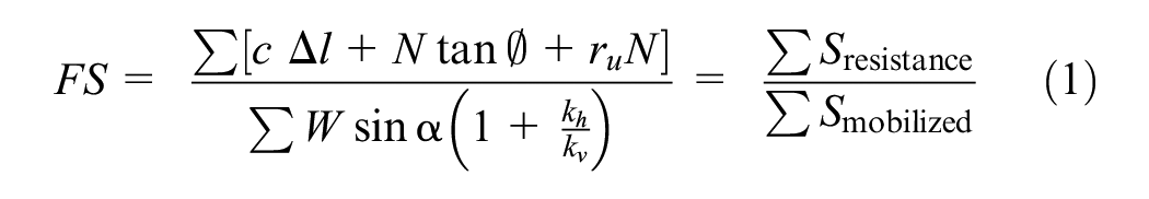
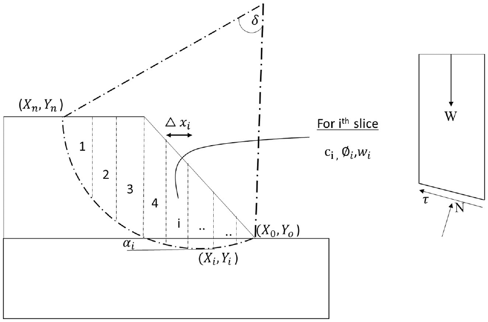
The available shear strength for a slope is determined by the base normal force, which is perpendicular to the slice base, whereas the driving force is calculated using the weight component parallel to the slice base. Figure 1 illustrates the dividing the sliding mass vertically into many slices, and also the free body diagram of a particular slice is shown. The FS is determined by dividing the total shear strength available along the slip surface by the sum of the mobilized shear driving forces. The FS is calculated using OMS considering pore water pressure ratio, as illustrated in Equation 1.
where c is cohesion, is slice base length, N stands for base normal (i.e., W, stands for pore water pressure ratio, represent angle of internal friction, W represents slice weight, is horizontal seismic coefficient, is the vertical seismic value, and is the slice base inclination. Conventionally, it is assumed that when FS is less than 1 slope is regarded as a fail.
Illustrative typical slope geometry.
Deterministic studies assume that soil attributes have fixed and known values, whereas probabilistic analyses take into account the uncertainty associated with soil properties within a slope. To account for this uncertainty, MCS and SS methods have been utilized in the current study for PA. The following subsection provides an illustration of the use of these methods in PA.
Random Field Modeling in Inherent Variability of Soil
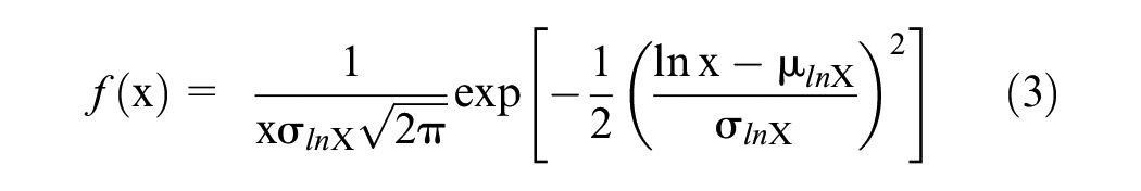
Soil properties can be viewed as stochastic variables used to gauge their variability or uncertainty. Despite their apparent uniformity, natural soil formations often reveal regional disparities attributable to the complex geological processes and historical loading events they have experienced (58). The random field, showing statistical homogeneity, has been discretized using different methods developed over time. In this work, the variability of soil within a statistically homogeneous layer is depicted by a one-dimensional lognormal field named F(X). This choice is made because of the unambiguous positivity of the soil parameter (59). The adoption of statistically homogeneous random fields is driven by the necessity to create a practical framework for numerical analysis, given the challenge of accurately representing the true physical homogeneity within natural soil layers. Through adjusting the random field parameters, such as correlation length and variance, in line with empirical soil data, we are able to incorporate the observed physical heterogeneity into our model. This ensures that the model accurately mirrors the real-world variability of soil characteristics. The process of calibrating these parameters, which is confirmed through comparison with independent datasets, significantly improves the model’s ability to predict within the parameters of the assumed framework. In this context, x is a lognormal random variable that exhibits mean value and standard deviation (SD) in a vertical direction which can be simulated using the expression as shown in Equation 2 (9, 38).
where and
are the mean and SD of ln(X), respectively; is the coefficient of variation representing the ratio of to the value; = a vector with unity components; is an n-dimensional standard Gaussian vector; L is a lower triangular matrix obtained through Cholesky decomposition, ensuring . Here, is the Pearson correlation matrix at different depths, calculated as , where and denotes the depth at two distinct locations and signifies the correlation length. Moreover, the PDF of a lognormal distribution is established using Equation 3.
Probabilistic Analysis
Several factors can introduce inaccuracy into a slope stability analysis, such as the random spatial distribution of soil properties, the difficulty of accurately determining stratigraphy below the surface, and mistakes in the computer models (60). Accounting for the inherent uncertainties associated with soil factors is a process that can be systematically addressed using probability theory and statistics. Within this study, the stochastic analysis of slope stability for road or rail embankments is performed, utilizing both MCS and SS techniques. These analyses are aided by the utilization of the “UPSS 3.0 Add-ins” tool embedded within the MS-Excel platform.
Monte Carlo Simulation
The MCS technique was initially developed in the 1940s by John von Neumann and Stanislaw Ulam (61), and is a numerical procedure for iteratively computing a mathematical or empirical operator with random or uncertain variables and predetermined probability distributions (62). A slope fails when it slides along any slip surface (i.e., a critical slip surface). Determining the overall failure probability (also known as the system ) along each potential slip surface is a challenging mathematical task (63). MCS is a robust technique to determine the desired level of on a slope in an efficient way compared with deterministic analysis. To ensure the desired level of accuracy in the estimation of , the minimum number of samples required in direct MCS should be at least ten times higher than the inverse of the desired accuracy level (i.e., 10/ ) (64–66). For instance, to attain an accuracy level of 0.001 using MCS, a minimum of 10,000 random samples should be generated. Let denote the N potential slip surface that are considered in the LEM analysis of slope stability. The slope failure occurs when any component (i.e., fails (i.e., FS < 1); then is frequently calculated by adding the total number of failed samples to the total number of random samples generated, as demonstrated in Equation 4. Subsequently, for the can be found using Equation 5.
where is the total number of cases where failure has occurred, N represents the total number of generated random samples and stands for the standard normal cumulative distribution function.
Subset Simulation
The SS is a more sophisticated variant of the MCS that utilizes conditional probability and the Markov chain Monte Carlo simulation (MCMCS) technique to accurately estimate small tail probabilities (67). It is a technique for quickly and effectively producing samples that match specified levels of failure probabilities in a progressive manner. To achieve the desired failure domain, this approach employs uniquely crafted Markov chains that generate conditional failure samples at intermediate events. This technique expresses the low level of probability for a rare failure event F into sequence of intermediate failure events with relatively higher conditional probability. To exemplify, let us examine the slope stability problem, where denotes the probability that the performance function T (i.e., the probability of FS less than fs or P [FS < fs]) falls below a specified threshold value t, or denoted as . These threshold values represent critical levels of the performance function T, where exceeding them indicates a degree of failure in slope stability. For instance, could represent the most critical threshold, while could denote a less severe failure condition. In this research, the target FS was considered to be less than 1.1 and threshold value greater than 0.909 (i.e., t = 1/FS), which was considered a failure sample. Therefore, if all samples have a threshold greater than 0.909, it is considered as a fail.
The SS methodology involves m + 1 steps, where the initial step employs a direct MCS to produce “N” unconditional samples. Subsequently, the remaining steps, consisting of m steps of MCMCS to generate conditional samples, can be calculated as , where N signifies the number of random sample produced in each step and is the conditional probability, which has been reported as 0.1 based on literature review (9, 67, 68). The sum of conditional samples produced by SS in “m” number of simulation levels is . Notably, the produced samples fall into m + 1 mutually exclusive and collectively exhaustive subgroups such as , determined by the intermediate threshold value. More specifically, the subgroup includes samples out of N samples. However, the last subgroup consist of all “N” samples. The is then calculated as shown in Equation 6.
where , k = 0; , k = 1, 2, …, m − 1; ; the occurrence probability of and it is considered as for k = 0,1, …, m − 1 and for k = m (69); represents the conditional failure probability of .
Details of Employed Computational Model
The intrinsic spatial variability of soil parameters, uncertainty in the underlying stratigraphy, and errors in the modeling are only a few examples of the elements that could potentially influence the results of a slope stability analysis. The amount of uncertainty associated with the soil parameter can be logically incorporated into slope analysis through the employment of ML. ML is a data-driven, empirical technique where a computer program “learns” from a dataset without being explicitly programmed with a problem and solution (70–72). Following the implementation of MCS and SS in the spreadsheet, three neural network-based models, RNN, LSTM, and BNN, have been investigated for the optimization of the worst failure condition. The theoretical background of the developed models is discussed in the following subsection.
Recurrent Neural Network
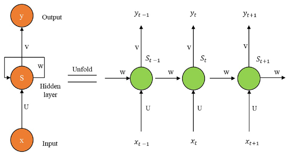
David Rumelhart’s research from 1986 served as the foundation for the RNN, which is a specialized type of neural network (73). RNNs are neural networks that are adept at modeling sequence data to comprehend the temporal dependencies and patterns within the data, making them particularly effective for tasks such as natural language processing, speech recognition, and time-series prediction. The RNN is different from the traditional neural network, also known as feed-forward neural network, in that it has an input layer, a hidden layer, and an output layer. It has the ability to utilize previous information to influence subsequent steps. In contrast, the looping mechanism of an RNN serves as a bridge to facilitate the transfer of information between steps. This information is encapsulated in the hidden state, serving as a representation of the preceding input and enabling the model to incorporate temporal dependencies in its learning process.
Here, xt stands for input, St and yt stand for and outer layer outputs at time t, respectively, and W, U, V indicates shared parameters of weight of inputs, weight of inputs at current state and weight of outputs at time t, respectively, as shown in Figure 2. The modeling techniques are defined by Equations 7 and 8.
where and are the respective bias vectors for the hidden and outer layers, and f(.) is an activation function like sigmoid function. As the time in travel increases, it can be seen that the in the front of the RNN expands, causing information loss and error accumulation in the in the back (74). In practice, when the time interval is prolonged and there is a vanishing gradient problem, the performance of RNN in maintaining memory can be compromised during training using the backpropagation through time. To overcome this issue, several variations of RNN have been developed.
Basic architecture of simple recurrent neural network (74).
Long Short-Term Memory
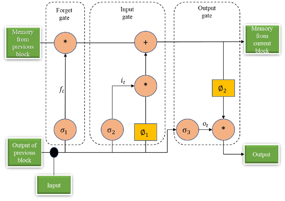
In 1997, Hochreiter and Schmidhuber introduced a novel variant of RNN called LSTM. The LSTM architecture was specifically designed to address the issue of vanishing gradients in traditional RNNs, enabling it to better handle long-term dependencies and to foretell the future events with greater accuracy (75). The LSTM architecture is designed to acquire knowledge of long-term dependencies among sequential data and time steps. Three different types of gates, namely, forget, input, and output, as well as a memory cell, are added by LSTM neurons. Additionally, it includes the sigmoid layer, the tanh layer, and the point-wise multiplication operation. The basic LSTM unit is shown in Figure 3. Notably, the , , and are the three sigmoid activation functions for forget, input, and output gates, respectively, and and are the hyperbolic tangent activation functions (tanh) as shown in Figure 3. Mathematically, the LSTM unit can be parameterized using Equations 9 to 13.
where , , , and illustrate the input, final output, cell state, forget gate, input gate and output gate vector, respectively, whereas , , , , , , and are the weight and bias of the forget gate, input gate, cell state and output gate, respectively.
Basic unit of long short-term memory.
Bayesian Neural Network
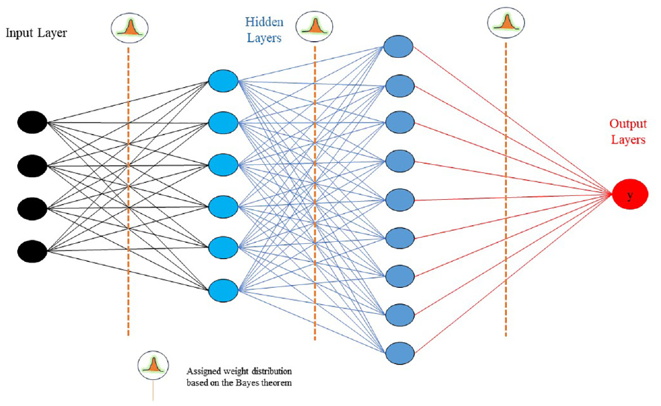
A BNN is a stochastic ANN that utilizes Bayesian inference in its development (76–78). Researchers came up with the BNN algorithm so they could take the best aspects of neural networks and probabilistic modeling and merge them (79). The purpose of this initiative is to make use of probabilistic modeling’s boundaries and guarantees, as well as the capability of neural networks to approximate universal functions. BNNs incorporate a probabilistic approach, whereas conventional neural networks use point estimates for their weights and biases. Instead, BNNs represent these parameters using posterior probability distributions (80, 81). The universal continuous function approximation capabilities of BNNs are similar to those of conventional neural networks. The learner in the Bayesian framework draws inferences about the posterior distribution across the parameters w of the model after analyzing the data k. The posterior distribution is given by Baye’s rule: , where is the likelihood of k given by the model with parameter w, and p(w) is the prior distribution over the parameters. The prediction of the model of the new set of data is then given by Bayesian model average (82). The basic architecture of BNN is presented in Figure 4.
Bayesian neural network architecture.
Illustrative Example
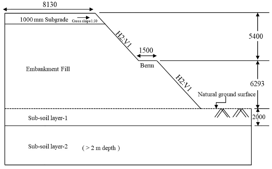
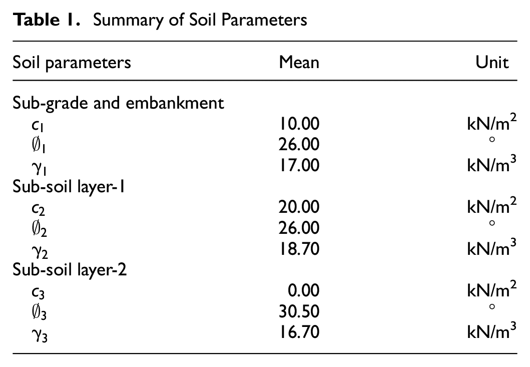
As an illustration, this section applies the PA of soil slope by MCS and SS with the use of MS-Excel “UPSS 3.0 Add-ins” to evaluate and . As illustrated in Figure 5, the embankment has a total height of 11.693 m, which comprises (a) a 1000 mm-thick prepared sub-grade and (b) an embankment fill that reaches a height of 10.693 m. The embankment has a slope angle of 26.6°, corresponding to an inclination ratio of 2H:1V. In this study, the soil layers situated below the natural ground surface have been divided into two distinct zones: sub-soil layer-1, with a depth of 2.0 m, and sub-soil layer-2, which lies beneath sub-soil layer-1 and has a depth greater than 2.0 m. It is noted that a berm width 1.5 m has been provided at a height of 5.4 m from the top of the embankment. In accordance with the recommendations made by the Research Designs & Standards Organisation (RDSO), the width of the berm should be at least 1.5 m on either side of the embankment for every maximum height of 6.0 m (measured from the top of the embankment) (83). It has been presumed that sub-soil layer-1 is predominately made up of silty sand and clay that ranges from moderate to low compressibility. On the contrary, the lower stratum is made up of silty sand that is combined with well-graded sand and silt. Table 1 illustrates the summary of soil parameters for the intended embankment. Particularly, in the sub-grade and embankment layer, the parameters are explicitly modeled using a 1-D lognormal random field, and stability of slope is examined by OMS. On the other hand, the parameters for the sub-soil layer-1 and sub-soil layer-2 are presumed to be deterministic. It should be emphasized that the horizontal seismic coefficient (kh) and the vertical seismic coefficient (kv) have been included in this analysis. For seismic condition, kh were set to 0.12 for zone-III and 0.14 zone-IV. However, in each zone kv = 0.5 × kh is taken into consideration. This line has been planned in accordance with the zoning map of India, as recommended furnished by RDSO (83). It is noted that influence of pore water pressure ratio (viz., , , and ) has also been addressed in this illustrative problem.
Slope geometry of 11.693 m-high embankment (all dimensions are in mm).
Summary of Soil Parameters
Soil parameters
Mean
Unit
Sub-grade and embankment
10.00
kN/m2
26.00
°
17.00
kN/m3
Sub-soil layer-1
20.00
kN/m2
26.00
°
18.70
kN/m3
Sub-soil layer-2
0.00
kN/m2
30.50
°
16.70
kN/m3
Deterministic Calculation
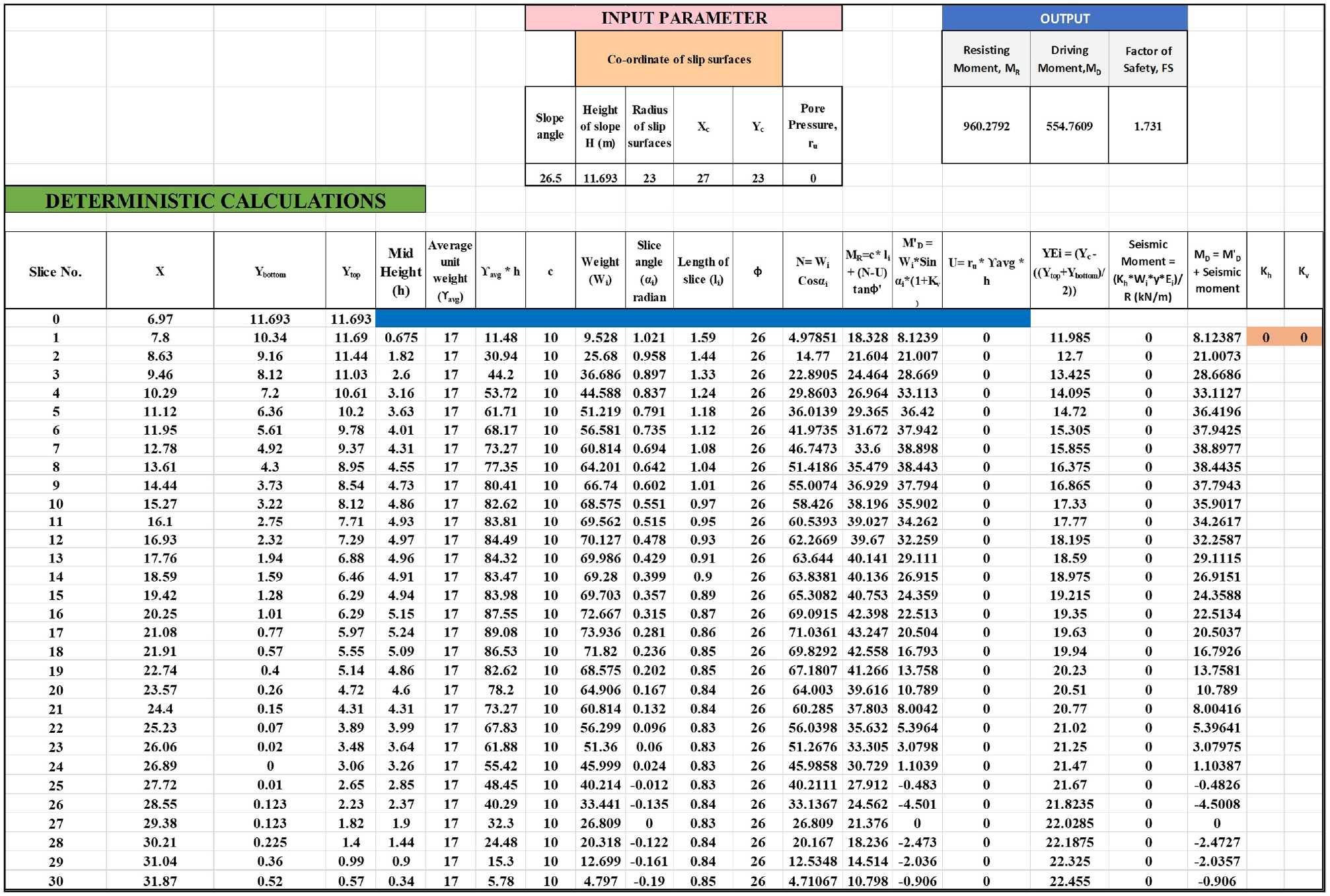
Deterministic analysis is a strategy to predict the behavior of system under conditions where input parameters remain constant or where uncertainty is not taken into account. In the current work, a deterministic analysis of a proposed case study of soil embankment has been reported using an Excel spreadsheet. To find the , OMS has been investigated, assuming circular slip surface with a defined center ( and radius (r). The calculation of for the given problem involved dividing the sliding mass into multiple slices, each characterized by its weight (, segment length , soil property (i.e., ), as well as an angle relative to the horizontal plane. Importantly, numerous trial-and-error approaches with all distinct combinations of and r for all potential slip surface by applying Equation 1 have been adopted for finding the .
Figure 6 illustrates the constructed deterministic spreadsheet, showcasing the determined value for an 11.693 m-high slope embankment. It is important to note that through numerous iterations the optimized ( and radius r of the proposed embankment were reported as and , respectively, defining a critical slip surface. It is essential to highlight that the presented worksheet has been developed under non-seismic condition with , and without considering soil uncertainty. However, the mean values slope soil parameters have been taken from Table 1. The output results (i.e., lowest FS) of the generated deterministic analysis are then validated with the Slope/W module in GeoStudio 2016, as can be seen in Appendix Figure A1(A). Subsequently, the results have since been validated, and the different seismic conditions (viz., kh = 0.12 and kh = 0.14) and conditions (viz., 0.0, 0.05, and 0.10) of the illustrative problem were addressed.
Generated deterministic Excel sheet.
In this study, a total thirty slices were divided in a deterministic calculation for the illustrative problem. As FS is dependent on the slip surface and soil property, the soil property is the most important input variable, as indicated in the section below.
Uncertainty Modeling
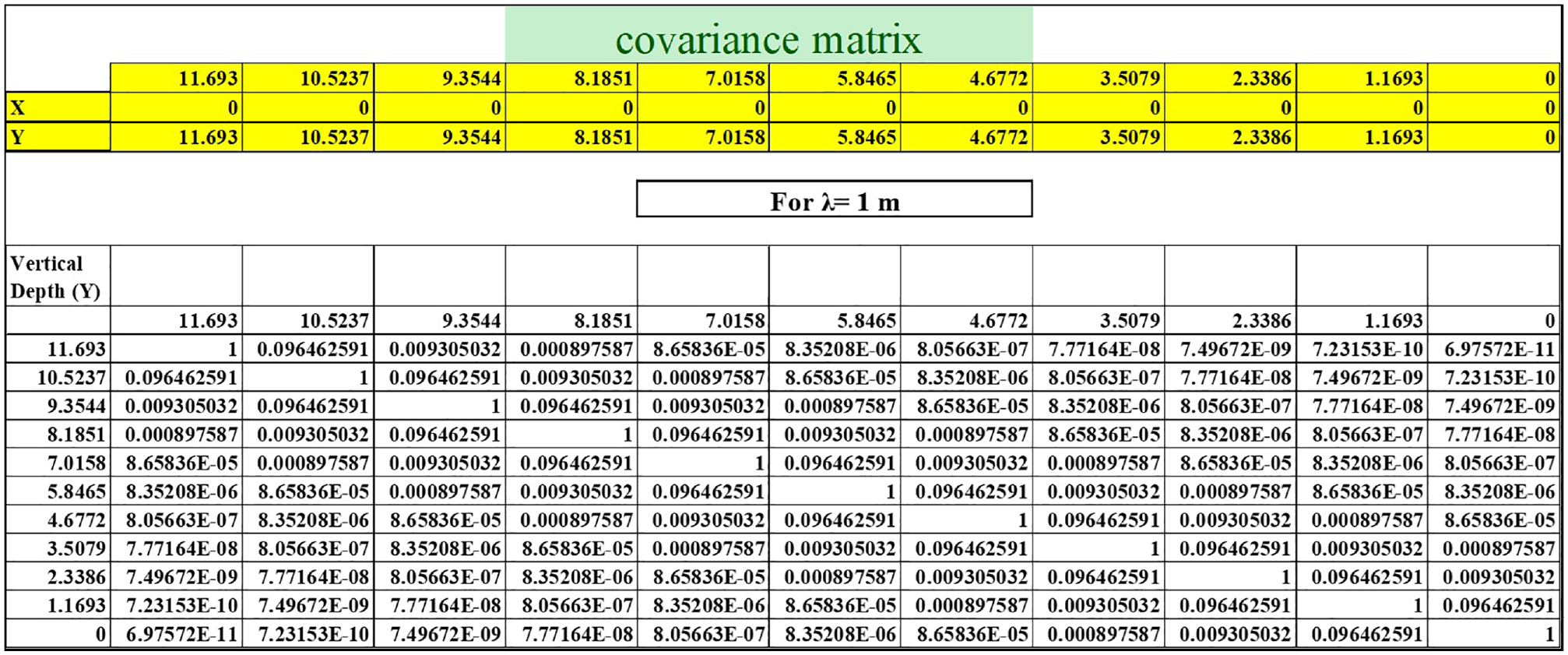
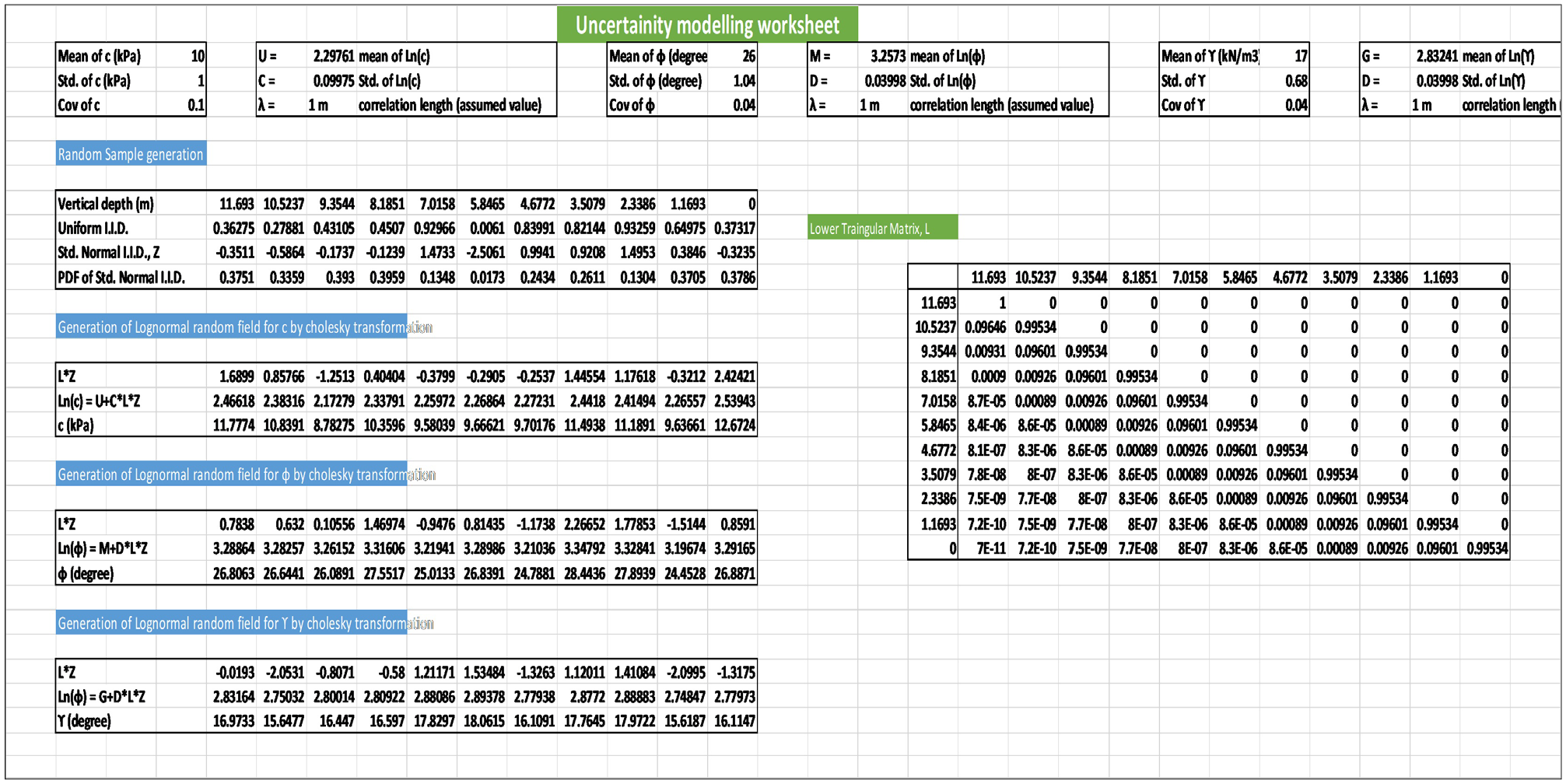
The uncertainty model (UM) spreadsheet is designed to generate random variables based on user-specified parameters. These parameters include factors such as the type of distribution, the deterministic correlation length, and the correlation structure. In this particular illustration, three parameters, namely , have been treated as random variables along with the depth and considered to be fully corelated. Uniform IID (independent and identically distributed) random samples are generated using the built-in “RAND ()” function in Excel, and then transformed into random samples of the desired distribution type (e.g., normal distribution or lognormal distribution). A homogeneous lognormal random field that has an exponentially falling correlation structure is used to describe the variability with depth. In this illustrative problem, the proposed embankment which is 11.693 m high was assumed to be divided into ten layers, each having a thickness 1.1693 m; a total of eleven uniformly IID random variables are required at eleven depths. Furthermore, the generated random variables are converted into standard Gaussian variables, and then PDFs using function “NORMINV ()” and “NORMDIST ()” in MS-Excel, respectively. For this particular analysis, a one-dimensional lognormal random field was created using Equation 2. The random variables used in the analysis are correlated with one another, and the correlation matrix or covariance matrix is illustrated in Figure 7 which is subjected to Cholesky factorization to create a lower triangular matrix (L). Once the “L” has been constructed, random variables are correlated using Equation 2 and reported in Figure 8 as a UM worksheet. Of note, the correlation length ( is set as 1.0 m, whereas the construction of “L” is performed using written MATLAB code. Additional details on the process of generating random samples can be found elsewhere (84). All details are comprehensively presented in the UM worksheet, including input parameters, random sample generation, the creation of a lognormal random field for , and the Cholesky matrix, shown in Figure 8.
Covariance matrix Excel worksheet.
Uncertainty modeling Excel worksheet.
Uncertainty Propagation
Following the execution of the deterministic calculation and the UM, the uncertainty propagation modeling is then utilized for the execution of the MCS and SS. This is achieved by linking the cell references of input variables in the deterministic calculation worksheet to the cell references of their corresponding random samples in the UM worksheet. By doing so, the values of uncertain parameters in the deterministic calculation become equivalent to the random samples generated in the UM worksheet, resulting in a failure probability that becomes random.
Results and Discussion
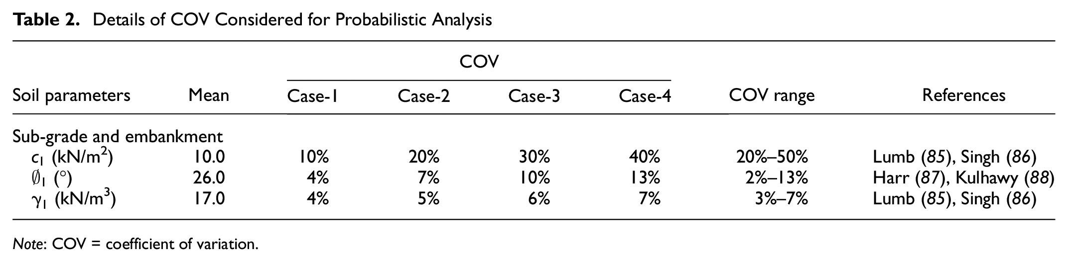
The results of the PA performed on an illustrative embankment with a height of 11.693 m using MCS and SS are presented in this section. The influence of the has also been explored, and its implications are discussed. Additionally, the range of coefficients of variation (COVs) was examined in accordance with the COVs of various soil properties based on the mentioned literature review in order to carry out PA. Table 2 illustrates the details of the COV range of proposed embankment. The parameter was fixed to 10%, 20%, 30% and 40% for case-1, case-2, case-3, and case-4, respectively. The COVs of and were fixed to 4% and 4%, 7% and 5%, 10% and 6%, and 13% and 7%, respectively. At each instance, the effect of (viz., 0.0, 0.05, and 0.10) and kh were set to 0.12 and 0.14 and categorized as Set-1 and Set-2, respectively. Subsequently, the worst probabilistic conditioning was investigated, and optimized through use of the ML technique. To accomplish this, three different types of neural network ML models, namely RNN, LSTM and BNN, were constructed.
Details of COV Considered for Probabilistic Analysis
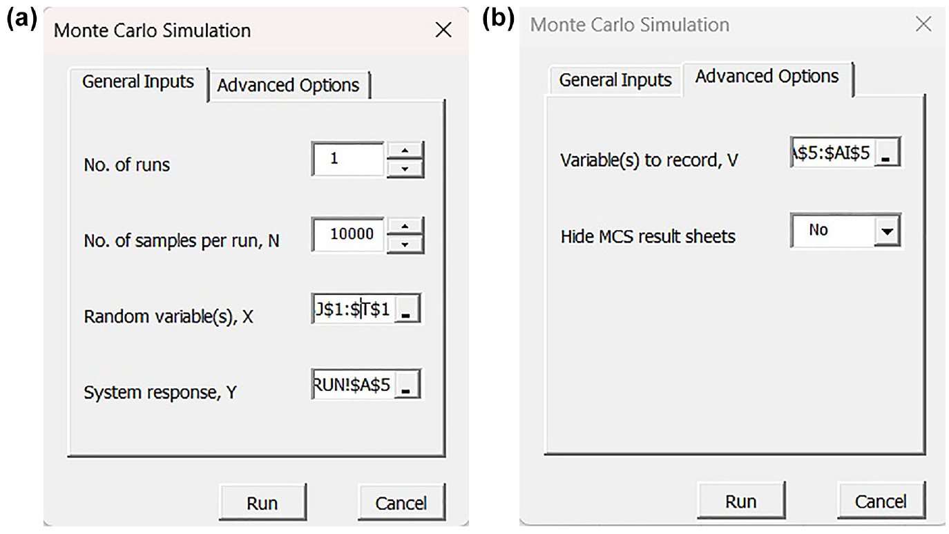
For the purpose of estimating , MCS and SS have been applied to this illustrative case. The following procedures need to be followed to accomplish the direct MCS through the UPSS dropdown toolbar: (a) click the add-ins in Excel; (b) select the direct MCS by clicking the “Simulation” UPSS dropdown menu in Excel; (c) select the no. of runs per sample (1 by default); (d) choose the sample size (1,000 by default); (e) select the standard normal IID variables from UM sheet; (f) select the system response, y (which can be defined as the reciprocal of FS, i.e., y = 1/FS) from UPM sheet; (g) to record the variable, select the “Advanced” option from the popup box; (h) to initiate the MCS simulation, click the Run option on the popup menu. Figure 9 depicts the direct MCS popup window box corresponding to general inputs and advanced options.
Direct Monte Carlo simulation (MCS) popup window box: (a) general inputs and (b) advance inputs.
In this illustrative case, four different combinations of COVs (i.e., case-1, case-2, case-3, and case-4) were investigated, as shown in Table 2. For the purpose of PA, 10,000 random samples have been generated for each scenario for the direct MCS simulation with in this instance. The and is computed by utilizing Equations 4 and 5, respectively.
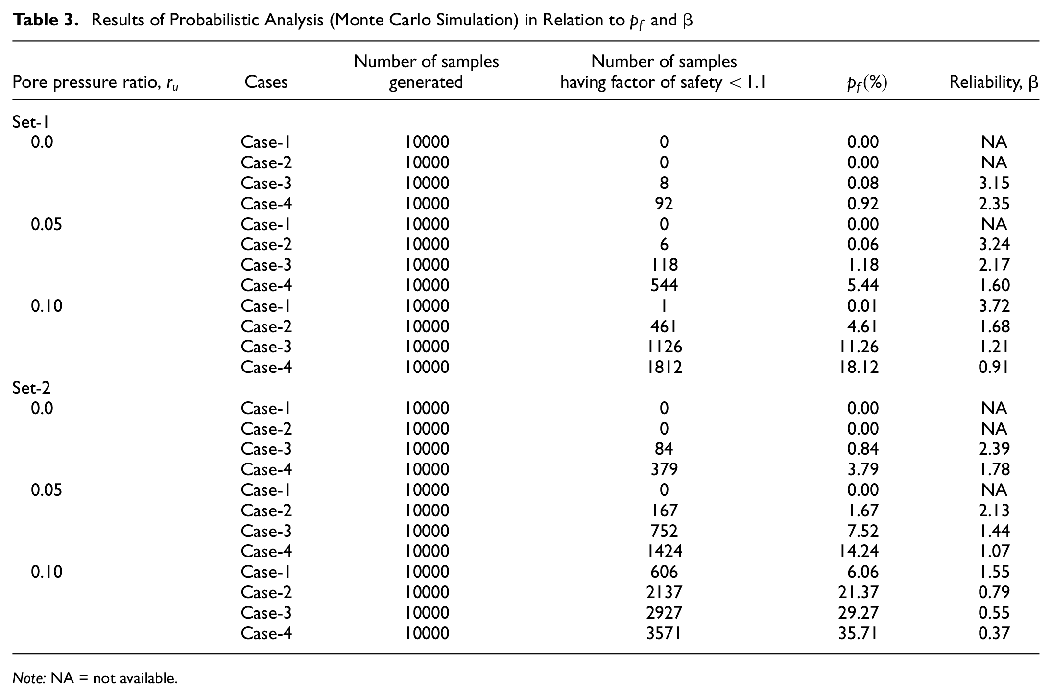
Table 3 shows the outcomes of the PA of the employed direct MCS for different values of the seismic coefficient, with the value showing the degree of failure probability of the illustrated problem in percentage. In each case, the values of were fixed to 0.0, 0.05, and 0.10, whereas the seismic coefficient was configured to be 0.12 and 0.14, and they were segmented as Set-1 and Set-2, respectively. In this context, it is important to note that the of the soil slope, determined based on the target FS value for seismic conditions, was less than 1.1 (51).
Results of Probabilistic Analysis (Monte Carlo Simulation) in Relation to and β
Pore pressure ratio,
Cases
Number of samples generated
Number of samples having factor of safety < 1.1
Reliability, β
Set-1
0.0
Case-1
10000
0
0.00
NA
Case-2
10000
0
0.00
NA
Case-3
10000
8
0.08
3.15
Case-4
10000
92
0.92
2.35
0.05
Case-1
10000
0
0.00
NA
Case-2
10000
6
0.06
3.24
Case-3
10000
118
1.18
2.17
Case-4
10000
544
5.44
1.60
0.10
Case-1
10000
1
0.01
3.72
Case-2
10000
461
4.61
1.68
Case-3
10000
1126
11.26
1.21
Case-4
10000
1812
18.12
0.91
Set-2
0.0
Case-1
10000
0
0.00
NA
Case-2
10000
0
0.00
NA
Case-3
10000
84
0.84
2.39
Case-4
10000
379
3.79
1.78
0.05
Case-1
10000
0
0.00
NA
Case-2
10000
167
1.67
2.13
Case-3
10000
752
7.52
1.44
Case-4
10000
1424
14.24
1.07
0.10
Case-1
10000
606
6.06
1.55
Case-2
10000
2137
21.37
0.79
Case-3
10000
2927
29.27
0.55
Case-4
10000
3571
35.71
0.37
Note: NA = not available.
Table 3 presents the results obtained from the MCS of the proposed illustrative slope embankment. Set-1 (i.e., kh = 0.12 and kv = 0.06) lies within the range of 0% to 18.12%, and Set-2 (i.e., kh = 0.14 and kv = 0.07) lies between 0% and 35.71%. This indicates that at higher seismic values, the chances of failure increase. Furthermore, it can be observed from Table 3 that higher β values correspond to lower values. It is observed that, value increases significantly from 0% to 0.92% for , 0% to 1.18% for , and 0.01% to 18.12% for when kh was set to 0.12. In a similar fashion, value increases from 0% to 3.79% for , 0% to 14.24% for , and 6.06% to 35.71% for when kh was set to 0.14. This is primarily because of the execution of a higher COV value and . Furthermore, a dramatic increase in value was observed when comparing Case-1 and Case-4 of Set-1 for , where the value increased from 0.01 to 18.12 (about 1,812 times). These findings suggest that an increase in COV leads to higher and lower β. In addition, the complementary cumulative distribution function (CCDF) plot for Set-1 and Set-2 with different COVs and the various conditions (i.e., , and ) has been given separately in the Appendix Figure A1(B) and Figure A1(C). This CCDF plot shows a relationship between P(Y > 1/FS) and driving variable (i.e., y = 1/FS). Notably, slope failure occurs when the driving variable y > 0.91, considering the seismic effect. It can be observed from the trend of the CCDF plot that when the COV value of the soil parameter increases, the likelihood of failure increases dramatically. Additionally, it can also be deduced from Figures A1(B) and A1(C), the increases correspond to an increase in seismic value.
SS-Based pf
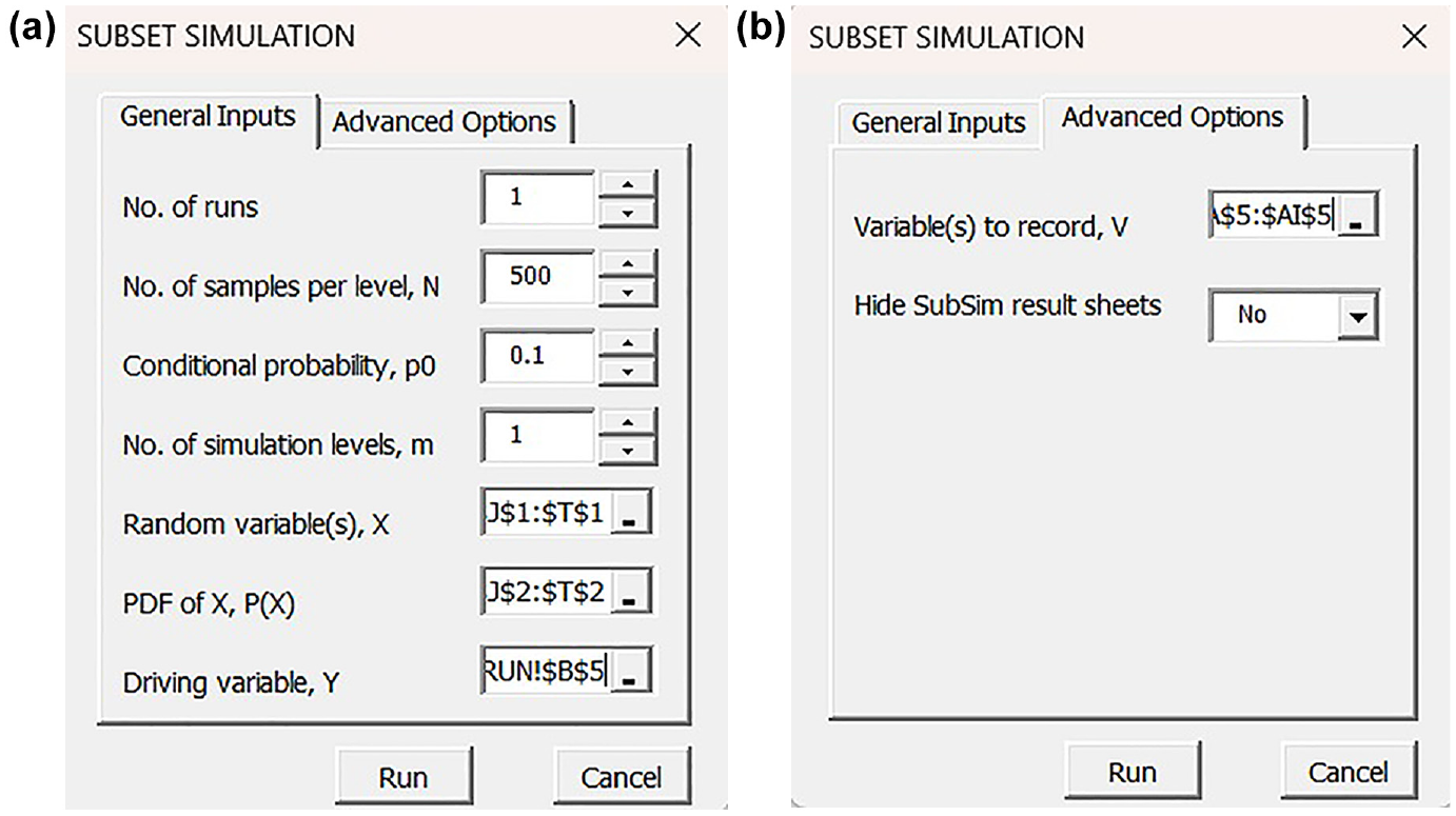
The SS is an advanced version of direct MCS, as has already been explained. SS was implemented for the same illustrative problem using the “Add-ins” option in Excel. The SS is performed by clicking the “simulation” button in the UPSS tool bar and choosing the “Subset simulation” option from the dropdown menu. Figure 10 depicts the general inputs as well as the advanced inputs section for the SS popup window, in which general inputs include the following seven keys: the number of runs (which has a default value of 1); the number of samples per level (N by default 200); the conditional probability ( which has a default value of 0.1); the number of simulation levels (m); the random variable; the PDF of the random variable; and the driving variable (Y, which is defined as the reciprocal of FS), whereas advance inputs options are for recording the variables.
Subset simulation popup window: (a) general inputs and (b) advance options.
In this investigation, SS is performed in each case by following conditions: = 0.1, N = 500, m = 3. Keep in mind that for each simulation run, the total number of samples is . This gives a total of samples, which include 450 samples at level 0 and 1, respectively, and 500 samples at level 2. The and β can be determined through the use of Equations 6 and 5, respectively.
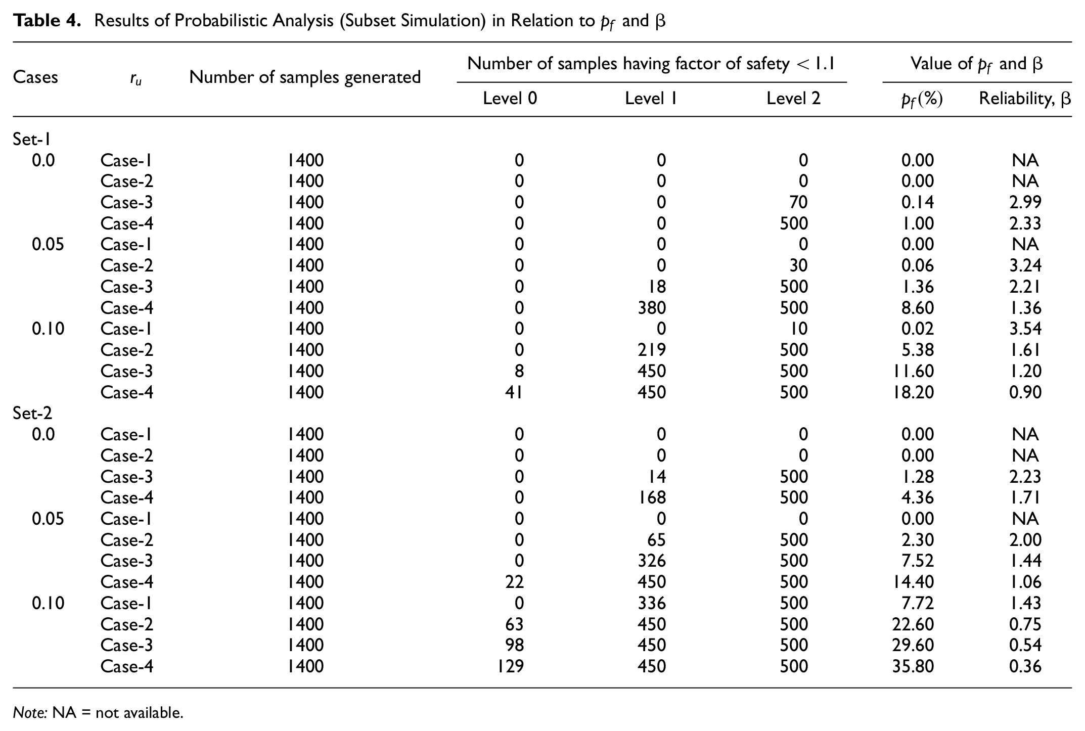
Referring to Table 4, the values for Set-1 and Set-2 fall somewhere in the range of (0%–18.2%) and (0%–35.8%), respectively. No failure is detected, when the value of is set to 0.0 in both sets of Case-1 and Case-2, and to 0.05 in both sets of Case-1. It is clearly seen from Table 4 for Set-1, the for lies in between 0% and 1%, and for lies in between 0% and 8.6% and for lies in between 0.02% and 18.2%. Furthermore, when kh was set to 0.14, the range of values were found to be 0%–4.36% for , 0%–14.4% for and 7.72%–35.8% for .
Results of Probabilistic Analysis (Subset Simulation) in Relation to and β
Cases
Number of samples generated
Number of samples having factor of safety < 1.1
Value of and β
Level 0
Level 1
Level 2
Reliability, β
Set-1
0.0
Case-1
1400
0
0
0
0.00
NA
Case-2
1400
0
0
0
0.00
NA
Case-3
1400
0
0
70
0.14
2.99
Case-4
1400
0
0
500
1.00
2.33
0.05
Case-1
1400
0
0
0
0.00
NA
Case-2
1400
0
0
30
0.06
3.24
Case-3
1400
0
18
500
1.36
2.21
Case-4
1400
0
380
500
8.60
1.36
0.10
Case-1
1400
0
0
10
0.02
3.54
Case-2
1400
0
219
500
5.38
1.61
Case-3
1400
8
450
500
11.60
1.20
Case-4
1400
41
450
500
18.20
0.90
Set-2
0.0
Case-1
1400
0
0
0
0.00
NA
Case-2
1400
0
0
0
0.00
NA
Case-3
1400
0
14
500
1.28
2.23
Case-4
1400
0
168
500
4.36
1.71
0.05
Case-1
1400
0
0
0
0.00
NA
Case-2
1400
0
65
500
2.30
2.00
Case-3
1400
0
326
500
7.52
1.44
Case-4
1400
22
450
500
14.40
1.06
0.10
Case-1
1400
0
336
500
7.72
1.43
Case-2
1400
63
450
500
22.60
0.75
Case-3
1400
98
450
500
29.60
0.54
Case-4
1400
129
450
500
35.80
0.36
Note: NA = not available.
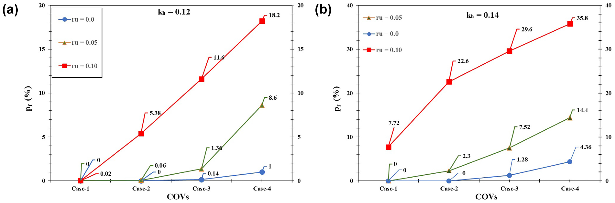
Figure 11 illustrates the relationship between (%) and COVs for different values of (i.e., 0.0, 0.05, and 0.10) using SS at two distinct seismic values (i.e., kh = 0.12 and kh = 0.14). It is evident from the figure that as values increase at both seismic values, increases sharply. Moreover, for a specific combination of and seismic values, increases significantly with an increase in the COVs of soil parameter. For instance, in Case-1, the value of was found to be 0.02 for = 0.10 and kh = 0.12, whereas for the same case, increased to 7.72 for = 0.10 and kh = 0.14. This observation suggests that the increase in is caused by the rise in seismic effect.
Trends between (%) and COVs at different condition: (a) kh = 0.12 and (b) kh = 0.14.
It is evident from Tables 3 and 4 that the results obtained through SS are nearly comparable to those obtained through MCS. However, the values obtained by SS are either equal to or higher than those obtained through direct MCS. It can be inferred that the same level of accuracy (in relation to ) can be achieved with SS using a smaller number of random samples (i.e., 1,400) compared with MCS, which generates 10,000 random samples. Additionally, SS takes less computation time (i.e., 16.37 s) compared with direct MCS (which takes approximately 1 min) to achieve the same degree of . The Appendix displays the CCDF plot for versus P(Y > 1/FS) for the illustrative slope using SS in Figures A1(D) and A1(E), respectively. A comparison of the CCDF plots obtained from the SS and MCS analyses indicates that the SS analysis can offer lower values. MCS reported a lower value of up to , whereas the SS analysis provides values up to .
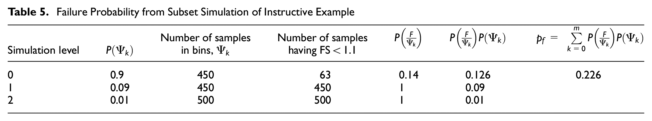
Referring to Table 4, the of Set-2 and the coefficient of = 0.10 for Case-2 have been selected as an illustrative example for estimating the using SS. Table 5. summarizes the procedure for estimating the of an instructive example. In a total of 1,400 SS samples, 1,013 were found to have FS less than 1.1, making them failure samples. These 1,013 samples are broken down as follows: sixty-three samples represent Level 0 (i.e., sixty-three samples failed in Level 0), 450 represent Level 1(i.e., all samples failed in Level 1), and 500 represent Level 2 (i.e., all sample failed in Level 2) of the simulation. With the use of these failure samples, for k = 0, 1, 2 is estimated as (63/450), (450/450), and (500/500) (see column 5). In addition, for k = 0, 1 and 2, the values are 0.9, 0.09, and 0.01 (see column 2), respectively. The can be estimated as or 22.6% that has been calculated by using Equation 6. Based on the resulting , β can be computed as which is equal to 0.75.
Failure Probability from Subset Simulation of Instructive Example
Simulation level
Number of samples in bins,
Number of samples having FS < 1.1
0
0.9
450
63
0.14
0.126
0.226
1
0.09
450
450
1
0.09
2
0.01
500
500
1
0.01
Computational Modeling
Following the completion of a PA using MCS and SS, the worst combination is chosen and subsequently optimized using ML. Remarkably, = 35.8% of SS has been proven to be the poorest possible combination (viz., Set-2, Case-4, and ). The run sheet of the worst combination of SS with an input random variable (i.e., c_11.693 to c_0, _11.693 to _0 and _11.693 to ) and FS are chosen to generate a total of 1,400 random data by using written MS visual basic code (VBA). Following the generation of 1,400 datasets at random, the employed models, namely, RNN, LSTM, and BNN were constructed by using all of the input and output parameters, followed by the random bifurcation of the training and testing datasets. To accomplish this, a total of 1,400 datasets are selected at random, normalized, and then divided in the following ratio: 70% (i.e., 980) are used for the training phase, and the remaining 30% (i.e., 420) are used for the testing phase. Of note, the bifurcation of datasets was done using written MATLAB code. It is also noted that the training datasets are used to create three neural network-based models, while the testing datasets are used to assess the model’s prediction precision in estimating the FS of an embankment that is 11.693 m high.
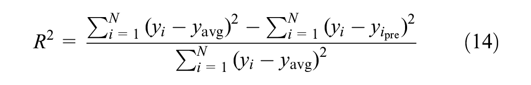
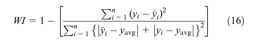
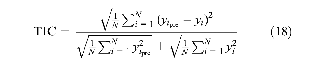
Following computational modeling, multiple evaluation metrics, namely determination coefficient (R2) (89), root mean square error (RMSE), Willmott’s index of agreement (WI), Legate and McCabes’s index (LMI), and Theli’s inequality coefficient (TIC) were determined, the mathematical expressions of which are given in Equations 14 to 18.
where N stands for the number of datasets, and is the mean of the actual and anticipated slope safety factor, respectively. and represent the actual and modeled predicted values of the ith values. It is absolutely necessary to have a solid comprehension that the values of these indices should match to their ideal values; details are already mentioned in the literature (90–92). Notably, conventionally evolution metrices should have the value 1 for R2, 0 for RMSE, 1 for WI, 1 for LMI and 0 for TIC (51, 92–95).
Performance Assessment
In this section, the performance of the employed neural network-based model is presented and discussed. The construction of the model involved utilizing a total of 980 datasets, as described above. The number of hidden neurons was studied for the RNN utilizing a trial-and-error methodology throughout a range that extended from 1 to 40; the optimal value of was found to be 20. The optimized RNN architecture consists of a hidden layer with twenty nodes, which is a simple RNN. The input shape has thirty-three time steps and one input feature, and the activation function used is ReLU (rectified linear unit). This is followed by two dense layers and an output layer. In addition, the “mean square error” function was used for best fitting, and the “Adam” function was used for optimization in the optimized RNN architecture. Similarly, in the LSTM neural network, a random hit-and-trial approach was used to investigate the first layer with various input nodes to achieve optimal performance. The optimized LSTM model consists of one input layer with thirty-three nodes, a LSTM hidden layer with fifteen neurons, an input shape of (33,1), and an activation function “ReLU”. This is followed by a dense layer and an output layer. Additionally, the “mean square error” function was used for best fit, and the “Adam” function was used for model optimization. It should be noted that in both the RNN and LSTM neural networks, 500 epochs and a batch_size of sixteen were used. For constructing the BNN model, first layer with thirty-three input parameters, one hidden layer with ten and an output layer were used. Subsequently, for best fit of the model, fifteen batch_size and 500 epochs were considered. It should be noted that for each model, different epochs between 300 and 500 were trialed, and the optimum epoch was found to be 500.
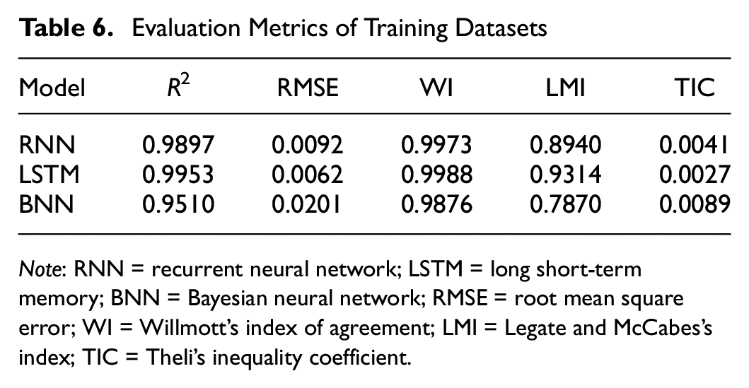
The prediction outcomes of the ML model were built for optimization of worst condition (i.e., = 35.8%) for estimating the FS. Here, evaluation metrics for the proposed model are illustrated in Table 6.
Evaluation Metrics of Training Datasets
Model
R2
RMSE
WI
LMI
TIC
RNN
0.9897
0.0092
0.9973
0.8940
0.0041
LSTM
0.9953
0.0062
0.9988
0.9314
0.0027
BNN
0.9510
0.0201
0.9876
0.7870
0.0089
Note: RNN = recurrent neural network; LSTM = long short-term memory; BNN = Bayesian neural network; RMSE = root mean square error; WI = Willmott’s index of agreement; LMI = Legate and McCabes’s index; TIC = Theli’s inequality coefficient.
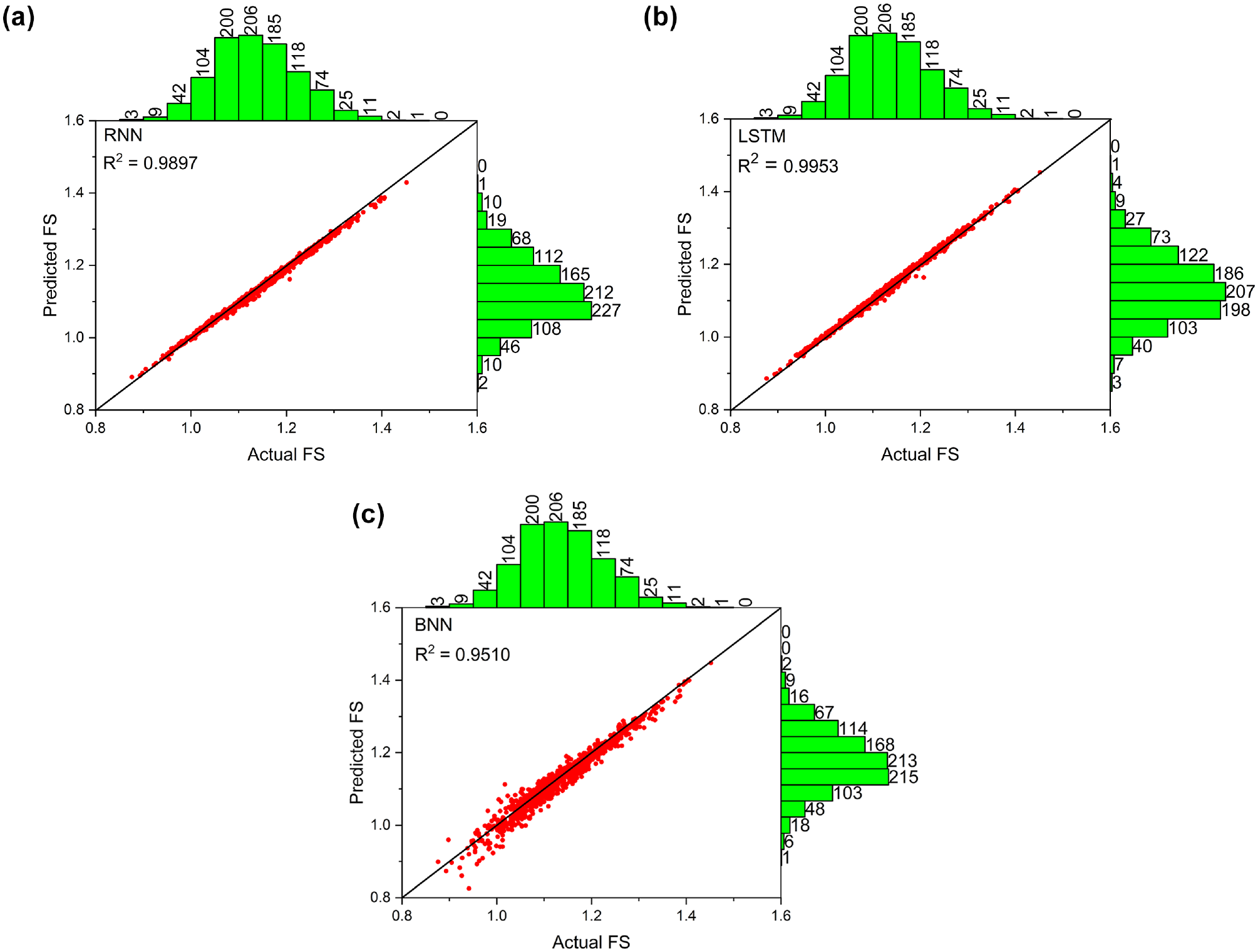
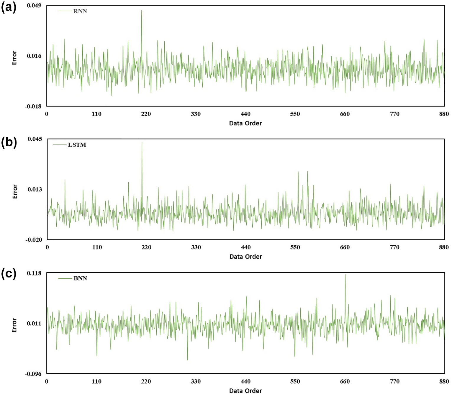
Of note, evaluation metrics have been employed to determine the model’s performance. From R2, the LSTM is 0.9953, which is higher than RNN (0.9857) and BNN (0.9510), showing better performance. From the RMSE and TIC, LSTM is 0.0062 and 0.0027 on the training phase, respectively, which is lower than 0.0092 and 0.0041 for the RNN, and 0.0201 and 0.0089 for the BNN model, respectively. Following a comparative analysis, it was concluded that the LSTM model demonstrated the most superior performance during the training phase. Additionally, it can be demonstrated that all the employed models obtained more than 95% accuracy (based on the R2 value), demonstrating a good fit with the datasets that have been obtained. However, to provide a clearer illustration of the fit, the marginal histogram and error plot of the actual and predicted FS values for each of the models that were used are presented in Figures 12 and 13, respectively.
Marginal histogram for training dataset: (a) RNN, (b) LSTM, and (c) BNN.
Error plot of (a) RNN, (b) LSTM and (c) BNN (Training phase).
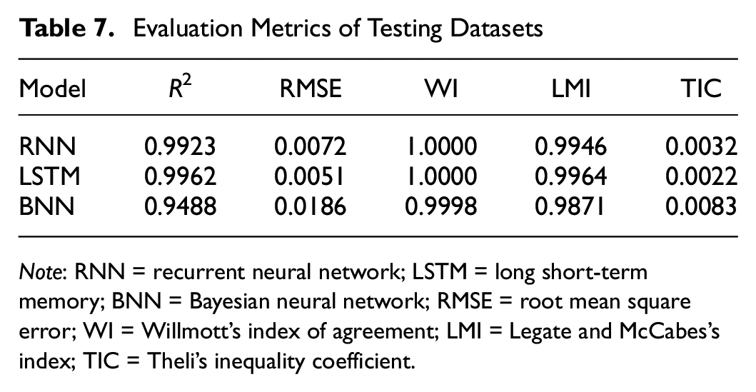
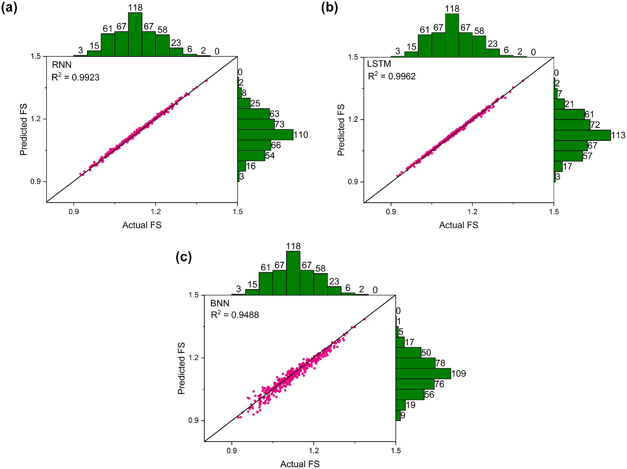
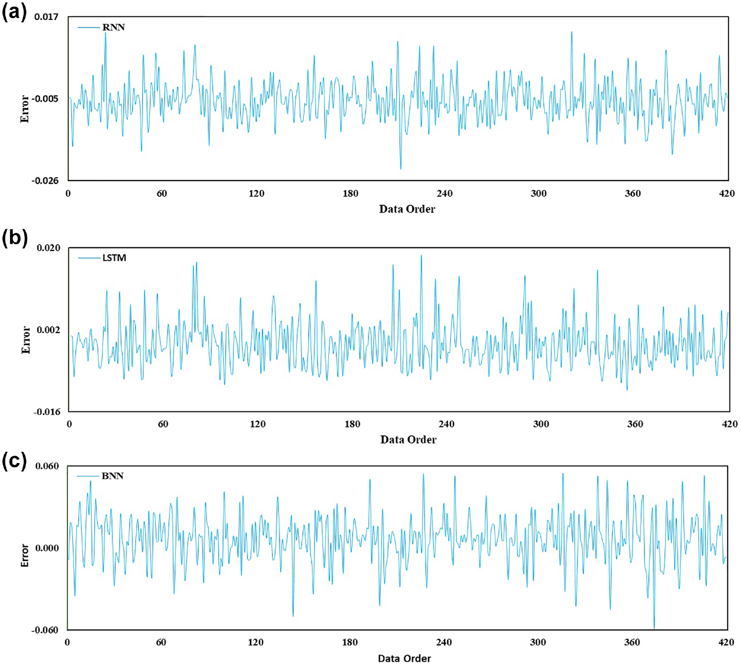
Following the building of the models, the unused datasets (a total of 420) were utilized during the testing phase of the models to determine their potential. Table 7 provides an instance of the evaluation metrics of the proposed-built models for testing datasets, and it can be concluded that throughout the testing phase, the suggested LSTM had the best precision in relation to R2 = 0.9962 and RMSE = 0.0051. In contrast, during the testing phase, the BNN model was shown to be the least effective across all evaluation metrics. However, the marginal histogram and error plot of the actual and predicted FS values in the testing phase for each of the models are presented in Figures 14 and 15.
Evaluation Metrics of Testing Datasets
Model
R2
RMSE
WI
LMI
TIC
RNN
0.9923
0.0072
1.0000
0.9946
0.0032
LSTM
0.9962
0.0051
1.0000
0.9964
0.0022
BNN
0.9488
0.0186
0.9998
0.9871
0.0083
Note: RNN = recurrent neural network; LSTM = long short-term memory; BNN = Bayesian neural network; RMSE = root mean square error; WI = Willmott’s index of agreement; LMI = Legate and McCabes’s index; TIC = Theli’s inequality coefficient.
Marginal histogram for testing dataset: (a) RNN, (b) LSTM, and (c) BNN.
Error plot of (a) RNN, (b) LSTM and (c) BNN (Testing phase).
Summary and Conclusion
It should be emphasized that carrying out a risk assessment of the rail or road embankment is essential for the smooth operation of the entire system. Thus, the current study presents a PA and reliability assessment of an illustrative example of soil slope using the MCS and SS techniques. To accomplish this, the MS-Excel spreadsheet software package “UPSS 3.0 Add-in” was used. The proposed illustrative embankment was 11.693 m high and had a soil slope of 2H:1V. In this study, two separate seismic coefficients, namely kh = 0.12 for Zone-III and kh = 0.14 for Zone-IV, which are in accordance with the current zoning map of India, were considered. Notably, seismic conditions were acquired as per the relevant guidelines by RDSO. Furthermore, values (i.e., 0.0, 0.05, and 0.10) were also taken into consideration. A PA was conducted using the MCS and SS techniques, and a range of COV levels were investigated. In the subsequent step, computational modeling was carried out utilizing three neural network-based models, namely, RNN, LSTM, and BNN, to optimize the worst of an 11.693 m-high soil slope. The experimental results lead to the following conclusion.
The deterministic method with OMS yielded a critical FS value of 1.731, and the critical slip surface was found to have coordinates of (27.0, 23.0) and a radius of 23.0 m. However, critical FS using GeoStudio SLOPE/W software was found to be 1.737, which is close to the deterministic calculation. The probabilistic and reliability analysis has been performed using the direct MCS and SS with the help of DM and UM sheet by considering the effect of uncertainty in soil parameters at . The results show that both methods provide appropriate solutions to estimate of 11.693 m-high embankment. Based on the analyses presented above, it was found that as COVs, , and kh values are increased, the of the slope also increases. Furthermore, the outcomes also suggest that the failure likelihood of a soil slope is affected not just by increasing and kh values, but also by variation in the COVs. In addition, the of soil slope increases significantly as the COVs of soil increases; this corresponds to the at kh = 0.12 from 0%–1% for , 0%–8.6% for and 0.02%–18.2% for . Similarly, at kh = 0.14 from 0%–4.36% for , 0%–14.4% for , 7.72%–35.8% for . This result demonstrates that as the COVs of soil parameters increase, the also increases dramatically. Moreover, it can be extrapolated from these results that as and seismic coefficient increases, also increases sharply. Of note, the aforementioned conclusions were reached by deducing the results based on the findings acquired using the SS approach. Particularly, presented CCDF trends using MCS and SS results also show that a rise in COV values, seismic coefficient and leads to an increase in .
The findings derived from the PA using SS are contrasted with those from MCS. The investigation reveals that both methods can be used to accurately estimate the of a soil slope. However, on comparison of the results obtained using SS for Set-1, Case-1, and = 0.10 (i.e., (%) = 0.02) with those obtained using direct MCS (i.e., (%) = 0.01), it was found that SS is superior in simulating low probabilities. In addition, the CCDF plot also demonstrates that SS can be produced at a low level of probability and can report up to , whereas MCS gives up to . Furthermore, achieving the appropriate level of accuracy in relation to , SS requires a smaller sample size compared with direct MCS, and this requires less computational time (i.e., 16.37 s) by SS in contrast to direct MCS (approximately 1 min).
From a computational modeling standpoint, the employed models, namely, RNN, LSTM, and BNN, were used for optimizing the worst scenario. Based on the experiment in the training and testing phases, LSTM found the best performing models (R2 = 0.9953 and RMSE = 0.0062) in the training phase as well as (R2 = 0.9962 and RMSE = 0.0051) in the testing phase for a particular type of optimization in soil slope among the three developed models in this work.
Supplemental Material
sj-docx-1-trr-10.1177_03611981241248166 – Supplemental material for Machine Learning-Aided Monte Carlo Simulation and Subset Simulation
Supplemental material, sj-docx-1-trr-10.1177_03611981241248166 for Machine Learning-Aided Monte Carlo Simulation and Subset Simulation by Md Shayan Sabri, Furquan Ahmad and Pijush Samui in Transportation Research Record
Footnotes
Author Contributions
The authors confirm contribution to the paper as follows: study conception and design: Md S. Sabri; data collection: Md S. Sabri; analysis and interpretation of results: Md S. Sabri, F. Ahmad; draft manuscript preparation: Md S. Sabri, F. Ahmad, P. Samui. All authors reviewed the results and approved the final version of the manuscript.
Declaration of Conflicting Interests
The author(s) declared no potential conflicts of interest with respect to the research, authorship, and/or publication of this article.
Funding
The author(s) received no financial support for the research, authorship, and/or publication of this article.
Data Accessibility Statement
Datasets have been provided in the manuscript.
Supplemental Material
Supplemental material for this article is available online.
References
1.
KaurA.SharmaR. K.Slope Stability Analysis Techniques: A Review. International Journal of Engineering Applied Sciences and Technology, Vol. 1, 2016, pp. 52–57.
2.
BurgessJ.FentonG. A.GriffithsD. V.Probabilistic Seismic Slope Stability Analysis and Design. Canadian Geotechnical Journal, Vol. 56, 2019, pp. 1979–1998.
3.
RukhaiyarS.AlamM. N.SamadhiyaN. K.A PSO-ANN Hybrid Model for Predicting Factor of Safety of Slope. International Journal of Geotechnical Engineering, Vol. 12, 2018, pp. 556–566.
4.
ZhouJ.LiE.YangS.WangM.ShiX.YaoS.MitriH. S.Slope Stability Prediction For Circular Mode Failure Using Gradient Boosting Machine Approach Based on an Updated Database of Case Histories. Safety Science, Vol. 118, 2019, pp. 505–518.
5.
ChengY. M.LansivaaraT.WeiW. B.Two-Dimensional Slope Stability Analysis By Limit Equilibrium and Strength Reduction Methods. Computers and Geotechnics, Vol. 34, 2007, pp. 137–150.
6.
RealeC.XueJ.PanZ.GavinK.Deterministic and Probabilistic Multi-Modal Analysis of Slope Stability. Computers and Geotechnics, Vol. 66, 2015, pp. 172–179.
7.
PhoonK.-K.KulhawyF. H.Evaluation of Geotechnical Property Variability. Canadian Geotechnical Journal, Vol. 36, 1999, pp. 625–639.
8.
JuangC. H.ZhangJ.ShenM.HuJ.Probabilistic Methods For Unified Treatment of Geotechnical and Geological Uncertainties in A Geotechnical Analysis. Engineering Geology, Vol. 249, 2019, pp. 148–161.
9.
WangY.CaoZ.AuS.-K.Practical Reliability Analysis of Slope Stability by Advanced Monte Carlo Simulations in a Spreadsheet. Canadian Geotechnical Journal, Vol. 48, 2011, pp. 162–172.
10.
ChowdhuryR. N.XuD. W.Geotechnical System Reliability of Slopes. Reliability Engineering & System Safety, Vol. 47, 1995, pp. 141–151.
11.
LiD.ZhouC.LuW.JiangQ.A System Reliability Approach For Evaluating Stability of Rock Wedges With Correlated Failure Modes. Computers and Geotechnics, Vol. 36, 2009, pp. 1298–1307.
12.
LiD.-Q.JiangS.-H.ChenY.-F.ZhouC.-B.System Reliability Analysis of Rock Slope Stability Involving Correlated Failure Modes. KSCE Journal of Civil Engineering, Vol. 15, 2011, pp. 1349–1359.
13.
ChristianJ. T.LaddC. C.BaecherG. B.Reliability Applied to Slope Stability Analysis. Journal Geotechnical Engineering, Vol. 120, 1994, pp. 2180–2207.
14.
YinY.Robust Optimal Traffic Signal Timing. Transportation Research Part B: Methodological, 2008.42: 911–924.
HekmatzadehA. A.ZareiF.JohariA.HaghighiA. T.Reliability Analysis of Stability Against Piping and Sliding in Diversion Dams, Considering Four Cutoff Wall Configurations. Computers and Geotechnics, Vol. 98, 2018, pp. 217–231.
17.
JohariA.GholampourA.A Practical Approach For Reliability Analysis of Unsaturated Slope By Conditional Random Finite Element Method. Computers and Geotechnics, Vol. 102, 2018, pp. 79–91.
18.
LiuY.ZhangW.ZhangL.ZhuZ.HuJ.WeiH.Probabilistic Stability Analyses of Undrained Slopes By 3D Random Fields and Finite Element Methods. Geoscience Frontiers, Vol. 9, 2018, pp. 1657–1664.
19.
LüQ.XiaoZ.ZhengJ.ShangY.Probabilistic Assessment of Tunnel Convergence Considering Spatial Variability In Rock Mass Properties Using Interpolated Autocorrelation and Response Surface Method. Geoscience Frontiers, Vol. 9, 2018, pp. 1619–1629.
20.
WangL.WuC.TangL.ZhangW.LacasseS.LiuH.GaoL.Efficient Reliability Analysis of Earth Dam Slope Stability Using Extreme Gradient Boosting Method. Acta Geotechnica, Vol. 15, 2020, pp. 3135–3150.
21.
DengZ.-P.PanM.NiuJ.-T.JiangS.-H.QianW.-W.Slope Reliability Analysis in Spatially Variable Soils Using Sliced Inverse Regression-Based Multivariate Adaptive Regression Spline. Bulletin of Engineering Geology and the Environment, Vol. 80, 2021, pp. 7213–7226.
22.
ZhouZ.LiD.-Q.XiaoT.CaoZ.-J.DuW.Response Surface Guided Adaptive Slope Reliability Analysis In Spatially Varying Soils. Computers and Geotechnics, Vol. 132, 2021, p. 103966.
23.
GohA. T. C.ZhangW. G.WongK. S.Deterministic and Reliability Analysis of Basal Heave Stability For Excavation in Spatial Variable Soils. Computers and Geotechnics, Vol. 108, 2019, pp. 152–160.
24.
FuZ.SuH.HanZ.WenZ.Multiple Failure Modes-Based Practical Calculation Model On Comprehensive Risk For Levee Structure. Stochastic Environmental Research and Risk Assessment, Vol. 32, 2018, pp. 1051–1064.
25.
GuoX.DiasD.CarvajalC.PeyrasL.BreulP.Reliability Analysis Of Embankment Dam Sliding Stability Using The Sparse Polynomial Chaos Expansion. Engineering Structures, Vol. 174, 2018, pp. 295–307.
26.
HicksM. A.LiY.Influence of Length Effect On Embankment Slope Reliability in 3D. International Journal for Numerical and Analytical Methods in Geomechanics, Vol. 42, 2018, pp. 891–915.
27.
KumarV.SamuiP.HimanshuN.BurmanA.Reliability-Based Slope Stability Analysis of Durgawati Earthen Dam Considering Steady and Transient State Seepage Conditions Using MARS and RVM. Indian Geotechnical Journal, Vol. 49, 2019, pp. 650–666.
28.
JiangS.-H.LiuX.HuangJ.Non-Intrusive Reliability Analysis of Unsaturated Embankment Slopes Accounting For Spatial Variabilities Of Soil Hydraulic and Shear Strength Parameters. Engineering with Computers, 2020, pp. 1–14.
29.
WangL.WuC.GuX.LiuH.MeiG.ZhangW.Probabilistic Stability Analysis of Earth Dam Slope Under Transient Seepage Using Multivariate Adaptive Regression Splines. Bulletin of Engineering Geology and the Environment, Vol. 79, 2020, pp. 2763–2775.
30.
MalkawiA. I. H.HassanW. F.AbdullaF. A.Uncertainty and Reliability Analysis Applied To Slope Stability. Structural Safety, Vol. 22, 2000, pp. 161–187.
31.
GriffithsD. V.HuangJ.FentonG. A.Influence of Spatial Variability on Slope Reliability Using 2-D Random Fields. Journal of Geotechnical and Geoenvironmental Engineering, Vol. 135, 2009, pp. 1367–1378.
32.
HuangJ.GriffithsD. VFentonG. A.System Reliability Of Slopes by RFEM. Soils Found, Vol. 50, 2010, pp. 343–353.
33.
RayA.BaidyaD.Probabilistic Analysis of A Slope Stability Problem. In Indian Geotech. Conf., 2011.
34.
JohariA.JavadiA. A.Reliability Assessment of Infinite Slope Stability Using The Jointly Distributed Random Variables Method. Scientia Iranica, Vol. 19, 2012, pp. 423–429.
35.
ChoS. E.First-Order Reliability Analysis of Slope Considering Multiple Failure Modes. Engineering Geology, Vol. 154, 2013, pp. 98–105.
36.
ZhangJ.HuangH. W.JuangC. H.LiD. Q.Extension of Hassan and Wolff Method For System Reliability Analysis of Soil Slopes. Engineering Geology, Vol. 160, 2013, pp. 81–88.
37.
JiangS.-H.LiD.-Q.CaoZ.-J.ZhouC.-B.PhoonK.-K.Efficient System Reliability Analysis of Slope Stability In Spatially Variable Soils Using Monte Carlo Simulation. Journal of Geotechnical and Geoenvironmental Engineering, Vol. 141, 2015, p. 4014096.
38.
LiD.-Q.XiaoT.CaoZ.-J.ZhouC.-B.ZhangL.-M.Enhancement of Random Finite Element Method In Reliability Analysis and Risk Assessment of Soil Slopes Using Subset Simulation. Landslides, Vol. 13, 2016, pp. 293–303.
39.
LuoN.BathurstR. J.JavankhoshdelS.Probabilistic Stability Analysis of Simple Reinforced Slopes By Finite Element Method. Computers and Geotechnics, Vol. 77, 2016, pp. 45–55.
40.
van den EijndenA. P.HicksM. A.Efficient Subset Simulation For Evaluating The Modes of Improbable Slope Failure. Computers and Geotechnics, Vol. 88, 2017, pp. 267–280.
41.
JiJ.ZhangC.GaoY.KodikaraJ.Effect of 2D Spatial Variability On Slope Reliability: A Simplified FORM analysis. Geoscience Frontiers, Vol. 9, 2018, pp. 1631–1638.
42.
JohariA.MousaviS.An Analytical Probabilistic Analysis of Slopes Based On Limit Equilibrium Methods. Bulletin of Engineering Geology and the Environment, Vol. 78, 2019, pp. 4333–4347.
43.
GuoX.DiasD.PanQ.Probabilistic Stability Analysis of An Embankment Dam Considering Soil Spatial Variability. Computers and Geotechnics, Vol. 113, 2019, pp. 103093.
44.
MahmoudiE.SchmüdderichC.HölterR.ZhaoC.WichtmannT.KönigM.Stochastic Field Simulation of Slope Stability Problems: Improvement and Reduction Of Computational Effort. Computer Methods in Applied Mechanics and Engineering, Vol. 369, 2020, p. 113167.
45.
SongL.YuX.XuB.PangR.ZhangZ.3D Slope Reliability Analysis Based On The Intelligent Response Surface Methodology. Bulletin of Engineering Geology and the Environment, Vol. 80, 2021, pp. 735–749.
46.
MaC.H.YangJ.ChengL.RanL.Research on Slope Reliability Analysis Using Multi-Kernel Relevance Vector Machine and Advanced First-Order Second-Moment Method. Engineering with Computers2021, pp. 1–12.
47.
HuC.QiX.LeiR.LiJ.Slope Reliability Evaluation Using An Improved Kriging Active Learning Method With Various Active Learning Functions. Arabian Journal of Geosciences, Vol. 15, 2022, p. 1059.
48.
ZengP.ZhangT.LiT.JimenezR.ZhangJ.SunX.Binary Classification Method For Efficient and Accurate System Reliability Analyses of Layered Soil Slopes. Georisk Assessment and Management of Risk for Engineered Systems and Geohazards, Vol. 16, 2022, pp. 435–451.
49.
ChuaiwateP.JaritngamS.PanedpojamanP.KonkongN.Probabilistic Analysis of Slope against Uncertain Soil Parameters. Sustainability, Vol. 14, 2022, pp. 14530.
50.
HeX.XuH.SabetamalH.ShengD.Machine Learning Aided Stochastic Reliability Analysis Of Spatially Variable Slopes. Computers and Geotechnics, Vol. 126, 2020, pp. 103711.
51.
BardhanA.SamuiP.Probabilistic Slope Stability Analysis of Heavy-Haul Freight Corridor Using A Hybrid Machine Learning Paradigm. Transportation Geotechnics, Vol. 37, 2022, p. 100815.
52.
SabriM. S.AhmadF.SamuiP.Slope Stability Analysis of Heavy-Haul Freight Corridor Using Novel Machine Learning Approach. Modeling Earth Systems and Environment2023, pp. 1–19.
53.
KumarK.SamuiP.ChoudharyS. S.State Parameter Based Liquefaction Probability Evaluation. International Journal of Geosynthetics and Ground Engineering, Vol. 9, 2023, p. 76.
54.
WangY.KeS.AnC.LuZ.XiaJ.A Hybrid Framework Combining LSTM NN and BNN for Short-Term Traffic Flow Prediction and Uncertainty Quantification. KSCE Journal of Civil Engineering, Vol. 28, 2024, pp. 363–374.
55.
JiaS.YueY.YangZ.PeiX.WangY.Travelling Modes Recognition via Bayes Neural Network with Bayes by Backprop Algorithm, In CICTP2020, 2020, pp. 3994–4004.
56.
WengP.JiaS.PeiX.YueY.Bayes Neural Network with a Novel Pictorial Feature for Transportation Mode Recognition Based on GPS Trajectories. In CICTP2021, 2021. pp. 1635–1645.
57.
AbdarM.PourpanahF.HussainS.RezazadeganD.LiuL.GhavamzadehM.FieguthP.CaoX.KhosraviA.AcharyaU. R.A Review of Uncertainty Quantification in Deep Learning: Techniques, Applications and Challenges. Information Fusion, Vol. 76, 2021, pp. 243–297.
58.
VanmarckeE. H.Probabilistic Modeling of Soil Profiles. Journal of Geotechnical and Geoenvironmental Engineering, Vol. 103, 1977, pp. 1227–1246.
59.
FentonG. A.GriffithsD. V.Risk Assessment in Geotechnical Engineering. John Wiley & Sons, New York, 2008.
60.
ZhuB.HiraishiT.PeiH.YangQ.Efficient Reliability Analysis of Slopes Integrating The Random Field Method and a Gaussian Process Regression-Based Surrogate Model. International Journal for Numerical and Analytical Methods in Geomechanics, Vol. 45, 2021, pp. 478–501.
61.
RogerE.Stan Ulam, John Von Neumann, and the Monte Carlo Method. Los Alamos Sciences1987, pp. 131–137.
62.
HemeidaM. G.AlkhalafS.SenjyuT.IbrahimA.AhmedM.Bahaa-EldinA. M.Optimal Probabilistic Location of DGs Using Monte Carlo Simulation Based Different Bio-Inspired Algorithms. Ain Shams Engineering Journal, Vol. 12, 2021, pp. 2735–2762.
63.
LiL.WangY.CaoZ.ChuX.Risk De-Aggregation and System Reliability Analysis of Slope Stability Using Representative Slip Surfaces. Computers and Geotechnics, Vol. 53, 2013, pp. 95–105.
64.
KarS. S.RoyL. B.Probabilistic Based Reliability Slope Stability Analysis Using FOSM. FORM, and MCS. Engineering Technology & Applied Scienc Research, Vol. 12, 2022, pp. 8236–8240.
65.
RobertC. P.CasellaG.Monte Carlo Statistical Methods. Springer, 1999.
66.
KangF.LiJ.-S.WangY.LiJ.Extreme Learning Machine-Based Surrogate Model for Analyzing System Reliability of Soil Slopes. European Journal of Environmental and Civil Engineering, Vol. 21, 2017, pp. 1341–1362.
67.
AuS.-K.WangY.Engineering Risk Assessment With Subset Simulation. John Wiley & Sons, 2014.
68.
AuS. K.ChingJ.BeckJ. L.Application of Subset Simulation Methods to Reliability Benchmark Problems. Structural Safety, Vol. 29, 2007, pp. 183–193.
69.
WangY.CaoZ., Expanded Reliability-Based Design of Piles in Spatially Variable Soil Using Efficient Monte Carlo Simulations. Soils Found, Vol. 53, 2013, pp. 820–834.
70.
JhaveriR. H.RevathiA.RamanaK.RautR.DhanarajR. K.A Review on Machine Learning Strategies for Real-World Engineering Applications. Mobile Information Systems, Vol. 2022, 2022, pp. 1–26.
71.
FrankM.DrikakisD.CharissisV.Machine-Learning Methods for Computational Science and Engineering. Computation, Vol. 8, 2020, p. 15.
72.
KumarD. R.SamuiP.BurmanA.Prediction of Probability of Liquefaction Using Soft Computing Techniques. Journal of The Institution of Engineers (India): Series A, Vol. 103, 2022, pp. 1195–1208.
73.
SalehK.HossnyM.NahavandiS.Contextual Recurrent Predictive Model for Long-Term Intent Prediction of Vulnerable Road Users. IEEE Transactions on Intelligent Transportation Systems, Vol. 21, 2019, pp. 3398–3408.
74.
BaiY.XieJ.LiuC.TaoY.ZengB.LiC.Regression Modeling for Enterprise Electricity Consumption: A Comparison of Recurrent Neural Network and its Variants. International Journal of Electrical Power & Energy Systems, Vol. 126, 2021, p. 106612.
75.
HochreiterS.SchmidhuberJ.Long Short-Term Memory. Neural Computation, Vol. 9, 1997, pp. 1735–1780.
76.
LampinenJ.VehtariA.Bayesian Approach for Neural Networks—Review and Case Studies. Neural Networks, Vol. 14, 2001, pp. 257–274.
77.
GoanE.FookesC.Bayesian Neural Networks: An Introduction and Survey. In: Case Studies in Applied Bayesian Data ScienceCIRM Jean-Morlet Chair, Fall2018, 2020, pp. 45–87.
78.
TitteringtonD. M.Bayesian Methods for Neural Networks and Related Models. Statistical Science2004, pp. 128–139.
79.
JospinL. V.LagaH.BoussaidF.BuntineW.BennamounM.Hands-on Bayesian Neural Networks—A Tutorial for Deep Learning Users. IEEE Computational Intelligence Magazine, Vol. 17 , 2022, pp. 29–48.
80.
CarlinB. P.LouisT. A.Empirical Bayes: Past, present and future. Journal of the American Statistical Association, Vol. 95, 2000, pp. 1286–1289.
81.
LiangF.Bayesian Neural Networks for Nonlinear Time Series Forecasting. Statistics and Computing, Vol. 15, 2005, pp. 13–29.
82.
IzmailovP.VikramS.HoffmanM. D.WilsonA. G. G.What are Bayesian Neural Network Posteriors Really Like?. In International Conference on Machine Learning, PMLR, 2021, pp. 4629–4640.
83.
M. O. F. Railways, Government of India Ministry of Railways Comprehensive Guidelines and Specifications for Railway Formation, (n. d.).
84.
AuS. K.CaoZ. J.WangY.Implementing Advanced Monte Carlo Simulation Under Spreadsheet Environment. Structural Safety, Vol. 32, 2010, pp. 281–292.
85.
LumbP.Application of Statistics in Soil Mechanics, Soil Mech. New Horizons (IK Lee, ed.), 1974.
86.
SinghA.How Reliable is the Factor of Safety in Foundation Engineering?, 1972.
87.
HarrM. E.Reliability-Based Design in Civil Engineering. Department of Civil Engineering, School of Engineering, North Carolina State, 1984.
88.
KulhawyF. H.On the Evaluation of Static Soil Properties. In Stab. Perform. Slopes Embankments II, ASCE, 1993. pp. 95–115.
89.
Tavana AmlashiA.Mohammadi GolafshaniE.EbrahimiS. A.BehnoodA.Estimation of the Compressive Strength of Green Concretes Containing Rice Husk Ash: A Comparison of Different Machine Learning Approaches. European Journal of Environmental and Civil Engineering, Vol. 27, 2023, pp. 961–983.
90.
RajaM. N. A.ShuklaS. K.Predicting the Settlement of Geosynthetic-Reinforced Soil Foundations Using Evolutionary Artificial Intelligence Technique. Geotextiles and Geomembranes, Vol. 49, 2021, pp. 1280–1293.
91.
LiZ.LiuF.YangW.PengS.ZhouJ.A Survey of Convolutional Neural Networks: Analysis. Applications, and Prospects. IEEE Transactions on Neural Networks and Learning Systems, 2021.
92.
RajaM. N. A.ShuklaS. K.An Extreme Learning Machine Model for Geosynthetic-Reinforced Sandy Soil Foundations. Proceedings of the Institution of Civil Engineers - Geotechnical Engineering, Vol. 175, 2022, pp. 383–403.
93.
YagizS.SezerE. A.GokceogluC.Artificial Neural Networks and Nonlinear Regression Techniques to Assess the Influence of Slake Durability Cycles on the Prediction of Uniaxial Compressive Strength and Modulus of Elasticity for Carbonate Rocks. International Journal for Numerical and Analytical Methods in Geomechanics, Vol. 36, 2012, pp. 1636–1650.
94.
KardaniN.AminpourM.RajaM. N. A.KumarG.BardhanA.NazemM.Prediction of the Resilient Modulus of Compacted Subgrade Soils Using Ensemble Machine Learning Methods. Transportation Geotechnics, Vol. 36, 2022, p. 100827.
95.
KhanK.IqbalM.JalalF. E.AminM. N.AlamM. W.BardhanA.Hybrid ANN Models for Durability of GFRP Rebars in Alkaline Concrete Environment Using Three Swarm-Based Optimization Algorithms. Construction and Building Materials, Vol. 352, 2022, p. 128862.
Supplementary Material
Please find the following supplemental material available below.
For Open Access articles published under a Creative Commons License, all supplemental material carries the same license as the article it is associated with.
For non-Open Access articles published, all supplemental material carries a non-exclusive license, and permission requests for re-use of supplemental material or any part of supplemental material shall be sent directly to the copyright owner as specified in the copyright notice associated with the article.