STC-PSSA: A New Model of Traffic Flow Forecasting Based on Spatiotemporal Convolution and Probabilistic Sparse Self-Attention

Abstract

Traffic flow forecasting is the foundation of the dynamic control and application of intelligent transportation systems (ITS). It is also of significant practical value in alleviating road congestion. Given the periodic and dynamic changes in trafﬁc ﬂow and the spatiotemporal coupling interaction of complex road networks, trafﬁc ﬂow forecasting is challenging and rarely yields satisfactory prediction results. To capture the dynamic spatiotemporal characteristics of traffic flow, a new model of traffic flow forecasting based on spatiotemporal convolution and probabilistic sparse self-attention (STC-PSSA) is proposed. It consists of a spatiotemporal graph convolution network (ST-GCN) module, a spatiotemporal convolution module (ST-Conv), and a probabilistic sparse attention module (PSSA). ST-GCN consists of the gated temporal convolutional network (G-TCN) and the graph convolution network (GCN), which are used to capture the temporal dependence and spatial correlation of the traffic flow, respectively. Multiple ST-GCNs are stacked to handle spatial features at various time levels. The ST-Conv captures intricate temporal dependence at the same location and dynamic spatial features at neighboring locations simultaneously. The PSSA combines dynamic spatiotemporal features and performs long-term forecasting efficiently. The experimental results demonstrate that the STC-PSSA model can accurately extract the dynamic spatiotemporal characteristics of traffic flow and outperforms the popular baseline methods in forecasting accuracy.

Keywords

data and data science artificial intelligence and advanced computing applications deep learning neural networks

With the rapid urbanization and the increasing complexity of traffic and road networks, accurate forecasting of traffic flows has become an indispensable part of Intelligent Transport Systems (ITS). Traffic flow forecasting aims to predict future traffic conditions based on historical traffic observations and to provide accurate spatiotemporal traffic flow forecasting services to alleviate traffic congestion. Figure 1 shows the common spatiotemporal relationship of traffic flows. Traffic data are recorded at fixed points in time and at fixed locations distributed in continuous space. The observations made at neighboring locations and time stamps are not independent but dynamically correlated with each other. Therefore, the key to solving such problems is to effectively extract the spatiotemporal correlations in the data. The bold line between two points represents their mutual influence strength: the darker the color of the line, the greater the influence. In the spatial dimension (Figure 1a), it can be found that different regions have different effects on point A, and even with the passage of time, the same region has different effects on point A. In the temporal dimension (Figure 1b), the traffic situation at point A will change according to different historical observation times. In conclusion, the correlations in traffic data on the highway network show strong dynamics in both the spatial and temporal dimensions. How to explore nonlinear and complex spatiotemporal data to discover the inherent spatiotemporal patterns and to make accurate traffic flow predictions is a very challenging issue.

Figure 1.

Spatial and temporal traffic flow diagram for the morning and evening peaks. The dots indicate residential neighborhoods, the stars indicate schools or companies. The correlation is stronger at the peak hour of 9 a.m. from home to work. The bold line between two points represents their mutual influence strength: the darker the color of line, the greater the influence: (a) spatial influence at different times; and (b) temporal influence between traffic flows.

It is challenging to concurrently capture the dynamic spatiotemporal elements in sophisticated traffic flow modeling using traditional machine learning techniques as those methods depend largely on characteristic engineering. The deep learning-based traffic flow forecasting methods are able to automatically capture features characterizing traffic flow properties and capture the dynamic spatiotemporal characteristics of traffic flow by analyzing time series data. As a result, deep learning strategies have been frequently applied to forecast traffic flow.

To capture the temporal and spatial characteristics of traffic flow, Ma et al. ( 1 ) proposed a traffic flow prediction model combining convolutional neural networks (CNN) and long short-term memory (LSTM) neural networks; CNN extracts local features through convolution and pooling operations. However, for non-Euclidean data such as road networks and meteorological data, the grid structure of CNNs makes it challenging to accurately model unstructured or irregular data, resulting in difficulties in capturing spatial features effectively. To address this limitation, Lv et al. ( 2 ) proposed the use of graph convolutional networks (GCN) to generate graph convolution modules capable of self-learning to capture the spatial features of traffic flows, but the convolution operation of GCN only considers the direct neighbor information of nodes, which is unable to adequately capture the remote associations between nodes and the spatiotemporal dependencies globally. Temporal GCN (T-GCN) ( 3 ) uses the feature matrix and adjacency matrix to capture temporal and spatial information, respectively, and extracts complex temporal dependencies and spatial features through gated recurrent unit (GRU) and GCN, respectively, but GRU may encounter the problem of gradient vanishing or gradient exploding, which makes it difficult to capture temporal dependencies in the far future. Attention-based spatiotemporal graph convolutional networks (ASTGCN) ( 4 ) combine spatiotemporal convolution and attention mechanisms to learn the features of traffic flow in time and space, respectively. However, the spatiotemporal convolution and attention mechanisms in ASTGCN primarily focus on local neighborhoods and relationships between nodes, lacking the ability to model long-term dependencies in traffic flow effectively. To acquire the spatiotemporal characteristics of traffic flow, spatiotemporal graph convolutional networks (STGCN) ( 5 ) combine gated temporal convolutional networks (TCN) and GCN, However, these models, despite taking into account the complex and dynamic spatiotemporal correlation of traffic flow, still need to be improved in model training efficiency as well as accuracy. Spatiotemporal synchronous graph convolutional networks (STSGCN) ( 6 ) construct a local spatiotemporal graph by connecting all the nodes in the previous and next moments to form a spatiotemporal adjacency matrix, and this connection only considers node connections in adjacent moments. However, STSGCNs do not consider node connections at more distant moments and correlations over time spans, which means that they cannot capture longer-term dependencies between nodes. Given the complex spatiotemporal correlation, dynamics, and uncertainty of traffic flow, the problem of traffic flow prediction faces major challenges in modeling, data preprocessing, and model training. This leads to a lack of effective extraction of the dynamic spatiotemporal attributes of traffic flow, resulting in low forecasting accuracy and difficulty in long-term forecasting ( 7 ).

To address the above traffic flow forecasting problem, a new model of traffic flow forecasting based on spatiotemporal convolution and probabilistic sparse self-attention (STC-PSSA) is presented. This model comprises a spatiotemporal graph convolution network (ST-GCN), a spatiotemporal convolution (ST-Conv), and a probabilistic sparse attention (PSSA) block. To capture the dynamic spatiotemporal features of traffic flow, this paper leverages the ST-GCN framework, which excels at capturing the dynamic relationships among graph nodes. By using ST-GCN, the model can effectively capture the evolving spatiotemporal patterns and interactions within the traffic network. Extracted features are fed into the ST-Conv subsequently to fully capture hidden spatiotemporal dependencies. The dynamic spatiotemporal features are fused, and the computational time complexity is reduced via the PSSA. In addition, a supervised and comprehensively trained graph convolution network is proposed. The network builds an adaptive adjacency matrix by learning traffic flow data, providing for effective extraction of dynamic spatial correlation among the traffic flow. Simultaneously, the STC-PSSA model integrates the stacked extended causal convolution network with the probabilistic sparse self-attention mechanism to better capture the dynamic spatiotemporal characteristics of traffic flow and effectively make long-range forecasting.

The main contribution of the paper is as follows:

A novel traffic flow forecasting model, STC-PSSA, is proposed, which combines spatiotemporal graph convolution, spatiotemporal convolution, and a probabilistic sparse attention mechanism. STC-PSSA can not only mine the dynamic spatiotemporal features of traffic flow more comprehensively to enhance forecasting accuracy but it can also lessen the model’s computational complexity.

A spatiotemporal graph convolutional network is set up to capture the temporal dependence of the traffic flow using extended causal convolutional networks with different granularities, and the construction of an adaptive adjacency matrix allows the dynamic spatial correlation of the traffic flow to be further captured. To analyze traffic flow’s spatiotemporal characteristics thoroughly, an additional spatiotemporal convolution block is employed to further capture the complex temporal dependence of traffic flow and the hidden spatial characteristics of neighboring locations.

A probabilistic sparse attention module is created to capture and learn the dynamic spatiotemporal characteristics of the traffic flow, and by adjusting the attention coefficients, the main attention is provided using a few key point products to efficiently perform long-term forecasting and improve the computational efficiency of the model.

Extensive experiments on two data sets show that the STC-PSSA model has better prediction performance than existing baseline methods.

Related Works

After years of continuous research and practice, traffic flow forecasting has achieved many research results in recent decades. In the field of time series, the autoregressive integrated moving average model (ARIMA) ( 8 ) and Kalman filter model ( 9 ) have been widely used in the field of traffic flow forecasting. These early methods studied the time series of traffic flow at each location separately and, in recent years, some studies have started to consider spatial information of traffic flow, such as similar transportation road networks ( 10 ) and external environmental information in different locations. However, these methods are still based on traditional time series models or machine learning models, which cannot capture the complex nonlinear spatiotemporal dependencies well.

For modeling the spatial aspects of traffic flow, the primary approaches include conventional convolutional networks, recurrent neural networks, graph convolution, and others. Traditional convolutional networks are limited to standard grid data and can only extract local features. GCN, on the other hand, can handle nonlinear graph-structured data and efficiently capture the global features of the data. Currently, there are two primary methods for GCN: the space domain-based method and the spectral domain-based method. The space domain-based method extracts node features by aggregating information from its neighbors. This approach is less computationally intensive, but selecting node neighborhoods for this method is extremely challenging. Niepert et al. ( 11 ) proposed a linear method for selecting the neighborhood of the central node and demonstrated that an accurate selection of the neighborhood can significantly boost the accuracy of forecasting. Li et al. ( 12 ) introduced GCN to the task of human action recognition by dividing each node’s surrounding area into separate subgroups and ensuring that each node has an equal number of subsets for efficient extraction of spatiotemporal features. The information on the neighborhood of a node is regarded as prior knowledge that remains fixed during the entirety of the training process. The spectral domain-based method aggregates neighborhood information for each node through spectral analysis. Its limitation is that GCN operates on the whole graph, and it has to process the whole graph every time, so the computational complexity is huge. Therefore, Bruna et al. ( 13 ) proposed a framework for generalized graph convolution that uses Laplace operators to improve the model’s computational effectiveness. Based on the framework of graph convolution, Song et al. ( 6 ) proposed a gated GCN for predicting traffic flow. The model captures the dynamic characteristics of the flow but does not recognize the dynamic temporal and spatial relationships of the flow. It is evident that a GCN-based model for traffic flow forecasting cannot be solely constructed using GCN. Other approaches, such as combining TCN or attention mechanisms, are required to simultaneously capture the spatiotemporal characteristics of traffic flow.

Spatiotemporal GCN is mainly based on recurrent neural networks (RNN), GCN, and attention mechanisms. When RNN is combined with GCN, the model gains the benefits of short-term memory, but its iterative training approach results in significant computational complexity, less efficient processing of long-term sequences, and a greater susceptibility to gradient vanishing or explosion. For instance, He et al. ( 14 ) designed an RNN-based graph convolutional recurrent unit model that filters inputs and hidden states concurrently to detect spatiotemporal correlations for predicting traffic flow. When dealing with spatiotemporal data, the recursive unit model of a graph volume product based on RNN mainly focuses on the dependence between the current time step and the adjacent time step. It pays more attention to local spatiotemporal correlation, but its ability to capture spatiotemporal characteristics in a long time range may be limited. Nevertheless, this network’s capabilities are inadequate for capturing spatiotemporal features that are crucial for long-term forecasting. In contrast, spatiotemporal graph convolution methods based on CNN can improve model training speed significantly. However, when the number of layers in the spatiotemporal graph convolution network is too deep, it can make feature extraction difficult. Additionally, LSTM is employed in CNN-based spatiotemporal graph convolution methods to process complex time series efficiently. Therefore, Bogaerts et al. ( 15 ) proposed a forecasting model that combines CNN-based spatiotemporal graph convolution with LSTM to capture synchronous dynamic spatiotemporal dependencies. The structure of the common spatiotemporal graph convolution is displayed in Figure 2. A spatiotemporal attention module makes the network automatically pay more attention to valuable information. The input adjusted by the attention mechanism is fed to the spatiotemporal convolution module. The spatiotemporal convolution module is composed of a graph convolution product in spatial dimension, which captures the spatial dependence from neighborhood and convolution along the time dimension, and makes use of the temporal dependence of neighboring time. The theory of graph volume product spectrum in spatial dimension extends convolution operation from grid-based data to graph structure data. The traffic network is essentially a graph structure, and the characteristics of each node can be regarded as the signal on the graph. To make full use of the topological characteristics of the traffic network, on each time slice, the graph convolution based on the spectrogram theory is used to directly process the signal, and the signal correlation of the traffic network in the spatial dimension is used. The spectral method transforms a graph into algebraic form to analyze its topological properties. After the convolution operation in the time dimension captures the adjacent information of each node in the space dimension, the standard convolution layer in the time dimension is further stacked, and the signal slice of the node is updated by merging the information of the adjacent time, as shown on the right of Figure 5.

Figure 2.

Spatiotemporal graph convolution structure.

Attention mechanisms are rapidly advancing and have widespread applications across multiple domains, including speech recognition, natural language processing, and image processing. As an example, Li and Lasenby ( 16 ) created a neural network for spatiotemporal characteristics that uses a self-attention mechanism to capture dynamic spatiotemporal correlations. Zhang et al. ( 17 ) put forward a graph-based multisensor traffic flow forecasting method that uses temporal attention to efficiently extract dynamic spatial features and intricate temporal dependencies. Zheng et al. ( 18 ) embedded the self-attention mechanism into a GCN to construct a traffic flow forecasting network that captures the dynamic spatiotemporal dependencies of traffic flows. Wen et al. ( 19 ) proposed a transformer-based deep neural network for traffic flow prediction, which introduces a bias vector in relative position coding and automatically learns the relative position information of time nodes when linearly mapping the feature tensor. Historical traffic state information is extracted by an encoder and the decoder autoregressively predicts future traffic states. Bui et al. ( 20 ) proposed a dynamic spatial transformer WaveNet network for multistep traffic flow prediction, in which the time convolution layer is used to capture long time series features and the transformer layer is used to capture dynamic spatial correlations.

While the aforementioned techniques use the self-attention mechanism to capture spatiotemporal dependencies, they generally disregard implicit relationships and concealed spatiotemporal features accumulated within the channel dimensions ( 21 ). This may reduce the model’s capability to capture spatiotemporal features. Therefore, when using the self-attention mechanism, it is very important to construct a good prediction model, and consider the implicit relationship and hidden temporal and spatial characteristics of traffic flow through the self-attention mechanism.

Building on previous research, the STC-PSSA model uses GCN, TCN, and probability-sparse self-attention mechanisms to simulate the facts of traffic flow by combining the topological graphical network structure of the traffic system and the traffic flow’s non-Euclidean data properties. The complex temporal dependencies and hidden dynamic spatial features of traffic flow are fully captured by TCN and GCN, correspondingly. Additionally, the model uses PSSA to further learn dynamic spatiotemporal features of traffic flow and reduce model computational complexity. At the same time, we use the gated fusion mechanism to adaptively fuse dynamic spatiotemporal features fed from the PSSA module. This reduces error propagation in the forecasting process and improves forecasting accuracy.

Methodology

Problem Definition

In this paper, graph $G = (V, E)$ is used to represent the topological structure of the traffic network, where $V$ represents a finite set of $| V | = N$ road nodes, and $E$ is a finite set of edges in a road network, which represents the connectivity between associated nodes. $A \in R^{N \times N}$ represents the adjacency matrix of graph $G$ . If $v_{i}, v_{j} \in V$ and $(v_{i}, v_{j}) \in E$ , $A_{ij}$ is 1, otherwise it is 0. In each time step $t$ , the graph $G$ has a dynamic feature matrix $X^{(t)} \in R^{N \times D}$ , $D$ is the feature dimension of each node. At the same time, to maintain consistency, the graph signal and the node characteristic matrix are used interchangeably.

Based on the above relationship, the purpose of traffic flow prediction is to predict the traffic flow in the future time period by giving the historical spatiotemporal traffic data of the past $S$ time period: $[X^{(t - S) : t}, G] \overset{f}{\to} X^{(t + 1) : (t + T)}$ , Among them, $X^{(t - S) : t} \in R^{N \times D \times S}$ , $X^{(t + 1) : (t + T)} \in R^{N \times D \times T}$ .

Framework of STC-PSSA

The STC-PSSA model’s overall structure is shown in Figure 3; it mainly consists of stacked spatiotemporal graph convolutional (ST-GCN) layers, a spatiotemporal convolutional (ST-Conv) module, and a PSSA module. ST-GCN contains G-TCN and GCN. Among them, G-TCN uses dilated causal convolutional networks at different levels of granularity to capture the traffic flow’s temporal dependence. Meanwhile, GCN extracts dynamic spatial features by constructing adaptive adjacency matrices. Each spatiotemporal graph convolutional layer is residually connected. The stacked ST-GCN block can capture the dynamic spatiotemporal features in historical traffic flow data. ST-Conv examines how multiple node features affect individual node features within the traffic flow’s topological structure and also uncovers the underlying temporal and spatial dependencies of ST-GCN inputs. PSSA combines dynamic spatiotemporal characteristics to effectively measure query sparsity. It uses a few key point products for primary attention to reduce the computational complexity of the model and contribute to long-term forecasting. In addition, the STC-PSSA model addresses the dynamic spatial correlations across various time periods by stacking numerous STC-PSSA layers to comprehensively capture the intricate temporal dependencies of traffic flows.

Figure 3.

Overall framework of STC- PSSA model.

ST-GCN Block

T-GCN Block contains gated time convolution (gated TCN) and graph convolution (GCN) product. Gated TCN consists of two parallel time convolution modules (TCN-a and TCN-b) to capture the time dependence of traffic flow. GCN further extracts the dynamic spatial characteristics of traffic flow by using an adaptive adjacency matrix. Through the stacked T-GCN Block, the dynamic temporal and spatial characteristics in the historical data of traffic flow are captured.

Gated Temporal Convolution Network

The G-TCN layer presented in this paper implements extended causal convolutional networks to capture the temporal dependency of nodes. By stacking convolutional layers, dilated causal convolutional networks obtain a large sensory field. In addition, dilated causal convolution slides the input into a specific step size and uses a non-recursive parallel computation approach to handle lengthy time sequences. This strategy enhances learning speed and mitigates the issue of gradient vanishing. In this paper, we use an extended causal convolution using kernel 2 and an expansion factor of $k$ . Inputs are chosen every $k$ intervals and the standard 1D convolution is employed for the selected inputs. Given a 1D sequence of inputs $x \in R^{T}$ and filter $f \in R^{K}$ , the dilated causal convolution operation of $x$ with $f$ at step $t$ is represented by Equation 1:

x * f (t) = \sum_{s = 0}^{K - 1} f (s) x (t - d \times s)

(1)

where $d$ is an expansion factor that controls the jump step size. The temporal convolution network layer’s receptive field grows exponentially as the expansion factors are stacked in increasing order. As a result, the expanded causal convolutional network presented in this paper can capture longer sequences using fewer layers, reducing computational demands while enhancing long-term forecasting accuracy.

In recurrent neural networks, gating mechanisms can effectively manage information flow through layers in the network’s temporal convolutional layers. The most basic gated temporal convolution mechanism consists of a single output gate, as illustrated in Figure 4. In G-TCN, TCN-a is mainly responsible for modeling the spatial dependencies between nodes by processing the features of nodes as well as the features of their neighboring nodes using graph convolution operations in the spatial dimension. This allows the information of the nodes to propagate and interact in the graph structure to capture the spatial relationships between the nodes. TCN-b, on the other hand, is mainly used to model the evolution of the nodes in the temporal dimension by processing the features of the nodes at different time steps by using the convolution operation on the temporal dimension, which permits the model to model the dynamics of the nodes’ features in time to capture the temporal dependencies between the nodes.

Figure 4.

The gated temporal convolutional network (G-TCN) framework.

Given the input $X \in R^{N \times D \times S}$ , the gating temporal convolution takes the following form:

h = g (ζ_{1} * X + b) ⊙ σ (ζ_{2} * X + c)

(2)

where

$ζ_{1}$ , $ζ_{2}$ , $b$ and $c$ represent the model parameters,

$⊙ denotes$ the product of elements,

$g (\cdot)$ serves as the activation function of the output, and

$σ (\cdot)$ functions as the Sigmoid function that governs the proportion of information conveyed to the subsequent layer.

G-TCNs are used to capture complex temporal relationships in the STC-PSSA model.

Adaptive Adjacency Matrix-Based Graph Convolutional Networks

GCN is a fundamental operation for deriving node characteristics from a given node’s structural information. GCN can aggregate and transform neighborhood information into smooth node signals and support multidimensional inputs. Let $X \in R^{N \times D}$ denote the input signal, $Z \in R^{N \times M}$ the output, $W \in R^{D \times M}$ the model parameter matrix, and $\tilde{A} \in R^{N \times N}$ the normalized adjacency matrix with self-circulation capability. GCN is defined as:

Z = \tilde{A} XW

(3)

The diffusion convolutional network (DCN) simulates the diffusion process of graphical signals with a restricted number of steps and is particularly applicable for spatiotemporal modeling. In this paper, by combining the diffusion convolution network with the graph convolution network, the generalized form of Equation 3 is obtained as follows:

Z = \sum_{k = 0}^{K} P^{k} X W_{k}

(4)

where $P^{k}$ stands for the transfer matrix’s power series, and $W_{k}$ is the parameter matrix. In an undirected graph, $P = A / rowsum (A)$ . In directed graph, the forward and backward diffusion process refers to the process of information dissemination from a given node in the direction of directed edges. Specifically, there exists a forward transfer matrix $P_{f} = A / rowsum (A)$ and a backward transfer matrix $P_{b} = A^{T} / rowsum (A^{T})$ . The combination of the forward and backward transfer matrices yields a diffusion graph convolutional network:

Z = \sum_{k = 0}^{K} P_{f}^{k} X W_{k 1} + P_{b}^{k} X W_{k 2}

(5)

Simultaneously, this paper proposes an adaptive adjacency matrix ${\tilde{A}}_{adp}$ that requires no prior knowledge and can be used to achieve end-to-end learning by stochastic gradient descent. The adaptive adjacency matrix can identify hidden spatial correlation by randomly initializing the two node embedding dictionaries with the learnable parameter $E_{1}$ , $E_{2} \in R^{N \times c}$ during the learning process. The adaptive adjacency matrix proposed in this paper is:

{\tilde{A}}_{adp} = SoftMax (ReLu (E_{1} E_{2}^{T}))

(6)

where $E_{1}$ is the source node embedding and $E_{2}$ is the target node embedding. The spatial dependency weights between the source and destination nodes are derived by multiplying $E_{1}$ and $E_{2}$ , the $ReLu$ activation function is used to eliminate weak links; and the $SoftMax$ function normalizes the adaptive adjacency matrix. Therefore, the transfer matrix, which hides the diffusion process, is the normalized adaptive adjacency matrix. Integrating predefined spatial correlation with self-learning concealed dynamic spatial characteristics, this paper introduces graph convolutional layers:

Z = \sum_{k = 0}^{K} P_{f}^{k} X W_{k_{1}} + P_{b}^{k} X W_{k_{2}} + {\tilde{A}}_{apt}^{k} X W_{k_{3}}

(7)

When no graph structure is provided, only an adaptive adjacency matrix is used to extract hidden and dynamic spatial features:

Z = \sum_{k = 0}^{K} {\tilde{A}}_{apt}^{k} X W_{k}

(8)

ST-Convolution Block

In a road network, each sensor detects data with a specific periodicity. For instance, on weekdays during the morning and evening peak periods, traffic volume substantially increases, resulting in generally reduced speeds. The concealed spatial properties of traffic flow are strongly correlated with the spacing between different sensors. The spatial characteristics of a road network, such as road layout, lane configuration, and intersection location, remain relatively stable in time. These factors contribute to the spatial characteristics of traffic flow and are not affected by short-term time changes.

As shown in Figure 5, a spatiotemporal convolution module consisting of three kernels is designed in this work. Three kernels corresponding to the temporal, spatial, and spatiotemporal perspectives capture spatiotemporal features extracted from the ST-GCN. This captures the influence of multiple node features on a single node feature in the topological graph structure of traffic flow. The temporal kernel captures the interdependency of traffic streams in the same place during different times, and the spatial kernel captures the spatial characteristics of traffic streams in adjacent places during the same time period. The first ST-Conv Block takes the output of the ST-GCN Block as input, and then each ST-Conv Block takes the output of the previous ST-Conv Block as input, that is, $X_{N}^{(l)} \in R^{C (l)} \times | V_{N} | \times T_{h}$ , $T_{h}$ represents the input of ST-Conv Block, and $C (l)$ represents the number of channels in $l$ layer. The output $X_{N}^{(l + 1)} \in R^{C (l + 1)} \times | V_{N} | \times T_{h}$ can be calculated from Equations 9 and 10.

H = LeakyReLU [ϖ_{st}^{[l + 1]} * X_{N}^{(l)}; ϖ_{t}^{[l + 1]} * X_{N}^{(l)}; ϖ_{s}^{[l + 1]} * X_{N}^{(l)};]

(9)

X_{N}^{(l + 1)} = LeakyReLU (ϖ_{o}^{[l + 1]} * H)

(10)

where

$ϖ_{t}^{[l + 1]}$ is the temporal kernel of $f \times 1$ ,

$ϖ_{s}^{[l + 1]}$ is the spatial kernel of $1 \times f$ , and

$ϖ_{st}^{[l + 1]}$ is the spatiotemporal kernel of $f \times f$ .

$LeakyReLU (\cdot)$ refers to the $Leaky$ modified linear unitary function while $* denotes$ the convolution operation. In this article, $f = 3$ . Finally, the outputs of the three convolutional kernels are combined and the convolution $ϖ_{o}^{[l + 1]}$ is used to compress the features while constraining the number of channels.

Figure 5.

Spatiotemporal convolution (ST-Conv) module framework.

PSSA Block

The form $(Q, K, V)$ is a common input to the self-attention mechanism. The dot product is calculated as follows:

A (Q, K, V) = Softmax (\frac{Q K^{T}}{\sqrt{d}}) V

(11)

where $Q \in R^{L_{Q} \times d}$ , $K \in R^{L_{K} \times d}$ , $V \in R^{L_{V} \times d}$ and $d$ denote the input query, key, value, and dimension, respectively. The attention factor $A (q_{i}, K, V)$ for the i-th query is presented as follows:

A (q_{i}, K, V) = \sum_{j} \frac{k (q_{i}, k_{j})}{\sum_{l} k (q_{i}, k_{l})} v_{j} = E_{p (k_{j} | q_{i})} [v_{j}]

(12)

where $q_{i}$ , $k_{i}$ and $v_{i}$ are the $i$ rows in $Q$ , $K$ and $V$ , respectively. $p (k_{j} | q_{i}) = k (q_{i}, k_{j}) / \sum_{l} k (q_{i}, k_{l})$ and $k (q_{i}, k_{l})$ use the asymmetric index kernel $(q_{i} k_{j}^{T} / \sqrt{d})$ .

The spatial complexity of calculating the point product $p (k_{j} | q_{i})$ with the self-attention mechanism is $O (L_{Q} L_{K})$ . However, in calculating the probabilistic sparse self-attention mechanism, the input lengths of the query and key are typically equal, denoted as $L_{Q} = L_{K} = L$ , resulting in a total time and space complexity of $O (L \ln L)$ . In addition, the probability-sparse self-attention mechanism combines probability sparsity and self-attention mechanisms, adjusting the attention coefficient based on the latter. This ensures that only select keys are important to each query, with a few key-dot products providing the primary attention and disregarding the others ( 22 ). This approach can effectively make long-term forecasts and conserve computing resources while maintaining model accuracy by indirectly integrating complex temporal dependencies and dynamic spatial features.

STC-PSSA employs $M (q_{i}, K)$ to indicate the sparsity of the i-th query, and $KL$ scatter measures the sparsity of the query as follows:

M (q_{i}, K) = \ln \sum_{j = 1}^{L_{K}} e^{\frac{q_{i} k_{j}^{T}}{\sqrt{d}}} - \frac{1}{L_{K}} \sum_{j = 1}^{L_{K}} \frac{q_{i} k_{j}^{T}}{\sqrt{d}}

(13)

Among them, the first term is the logarithm and exponent of $q_{i}$ on all bonds, and the second term is their arithmetic average. According to the aforementioned principle, the probabilistic sparse self-attention mechanism is achieved:

A (Q, K, V) = Softmax (\frac{\bar{Q} K^{T}}{\sqrt{d}}) V

(14)

where $\bar{Q}$ represents a sparse matrix with the same dimensions as $q$ , which consists of only the first $u$ queries under the sparsity evaluated by $M (q, K)$ . $u = c \cdot \ln L_{Q}$ is determined by a constant sampling factor $c$ . Therefore, the complexity of the probabilistic sparse self-attention mechanism is only $O (\ln L_{Q})$ per query. In the multihead perspective, the mechanism can generate distinct sparse query-key pairs for each head, thereby circumventing substantial information loss.

Loss Function

The purpose of training is to minimize the error between actual traffic speed and predicted traffic speed in a road network. In this paper, the mean square error (MSE) is used as the loss function. The actual traffic speed and predicted traffic speed of different sections are expressed by $y_{i}$ and ${\hat{y}}_{i}$ , respectively, and n is the number of samples. Therefore, the loss function of STC-PSSA model is as follows:

MSE = \frac{1}{n} \sum_{i = 1}^{n} {(y_{i} - {\hat{y}}_{i})}^{2}

(15)

Experiment

Data Description

In this work, the predictive performance of the STC-PSSA model is validated on the public transit data sets METR-LA and PEMS-BAY ( 23 ). METR-LA consists of traffic speed statistics recorded by 207 sensors on freeways in Los Angeles County over a four-month period. PEMS-BAY includes traffic speed information recorded by 325 sensors on transportation roadways in the San Francisco Bay Area during a six-month period. Both the METR-LA and PEMS-BAY record the detection position, date, and data type. The experimental data set details are presented in Table 1.

Table 1.

Description of the Experimental Data Sets

Data	METR-LA	PEMS-BAY
Type	Sequentially	Sequentially
Attribute	Speed	Speed
Location	Highways of Los Angeles	The Bay Area
Edges	1,515	2,369
Time steps	34,272	52,116
Nodes	207	325

Since the METR-LA data set lacked a few data, the experiment used linear interpolation to fill in the missing values. The data is subjected to min-max normalization before being fed into the forecasting model, limiting its range to [0, 1]. The normalized formula is:

X_{i}^{norm} = \frac{x_{i} - x_{\min}}{x_{\max} - x_{\min}}

(16)

where

$x_{i}$ indicates the i-th source data,

$x_{\min}$ and $x_{\max}$ stand for the minimum and maximum values of the source data, respectively, and

$X_{i}^{norm}$ denotes the normalized input data.

Parameter Setting

This paper uses an 8-layer STC-PSSA network with an expansion factor sequence of 1, 2, 1, 2, 1, 2, 1, 2. Meanwhile, the graph convolutional network layer employs Equation 5 and the diffusion step is $K = 2$ . The STC-PSSA is trained using an Adam optimizer with an initial learning rate of 0.001 and a dropout rate of $p = 0.3$ . In the experiment, the data set is chronologically divided into training, test, and validation sets in the ratio of 7:2:1 for predicting traffic flow forecasts for 15 min, 30 min, and 60 min. In this paper, traffic flow for 12 consecutive time steps of the past hour is used to predict future traffic flow for 12 consecutive time steps of the next hour. To analyze the experimental results and evaluate the model’s forecasting performance, this paper uses the mean absolute error (MAE), root mean square error (RMSE), and mean absolute percentage error (MAPE) to evaluate the discrepancy between the actual traffic flow speed and the forecasting results.

MAE = \frac{1}{N} \sum_{i = 1}^{N} | y_{i} - {\hat{y}}_{i} |

(17)

RMSE = \sqrt{\frac{1}{N} \sum_{i = 1}^{N} {(y_{i} - {\hat{y}}_{i})}^{2}}

(18)

MAPE = \frac{100}{N} \sum_{i = 1}^{N} | \frac{y_{i} - {\hat{y}}_{i}}{y_{i}} |

(19)

where $N$ indicates the number of observations, and $y_{i}$ and ${\hat{y}}_{i}$ represent the actual and predicted traffic flows, respectively. The STC-PSSA model’s forecasting is deemed better when MAE, RMSE, and MAPE have smaller predicted values.

Baselines

This paper compares STC-PSSA with the following models:

(1) HA ( 23 ): historical average. The average value of historical and current traffic flow is involved as the prediction value for the next step. In the baseline method, the average of the past 12 time slices in the same period as a week ago is used to predict the current time slice.

(2) VAR ( 24 ): vector autoregression. In the baseline method, (p, d, m) is set to (1, 1, 1).

(3) SVR ( 25 ): an extension of the support vector machine (SVM) classification in regression problems. The insensitive loss coefficient ε is set as 0.1 and the penalty factor C is set as 1.0 according to the grid search method.

(4) FNN ( 25 ): feedforward neural network. The neural networks are L2-regularized and have two hidden layers.

(5) ARIMA ( 26 ): autoregressive integrated moving average. A popular model used in time series prediction. The orders of autoregression, difference, and moving average are the three crucial parameters for the ARIMA model. In the baseline method, (p, d, q) is set to (4, 1, 1).

(6) FC-LSTM ( 26 ): fully connected long short-term memory, which is a classic RNN for learning time series and making predictions by fully connected neural networks. In the baseline method, the number of hidden layers is set to 1 and the number of hidden units is set to 64.

(7) WaveNet ( 27 ): abbreviation for an improved WaveNet network for multistep-ahead wind energy forecasting. CNN for predicting sequence data. The number of stacked layers in this model is set as eight with the dilation rate [1, 2, 1, 2, 1, 2, 1, 2, 1, 2] and the hidden dimension is set as 64.

(8) Graph WaveNet ( 28 ): abbreviation for Graph WaveNet for deep spatiotemporal graph modeling, which is constructed by the GCN and the gated temporal convolution (gated TCN) layer. Each layer in this model contains a gated TCN and a spatial GCN. The number of stacked layers in this model is set as eight with the dilation rate [1, 2, 1, 2, 1, 2, 1, 2, 1, 2] and the hidden dimension is set as 64.

(9) STGCN ( 6 ): spatiotemporal graph convolutional network, which employs the graph convolutional layers and convolutional sequence layers. The number of spatiotemporal cells is set as two and the hidden dimension is set as 64.

(10) ASTGCN ( 4 ): attention-based spatiotemporal graph convolutional networks, which employ the attention mechanism to capture the spatiotemporal dynamic correlations. Similar to STGCN, there are two spatiotemporal cells in this model and the hidden dimension is set as 64.

(11) STSGCN ( 5 ): spatiotemporal synchronous graph convolutional networks, which captures the localized spatial and temporal correlations individually. The size of spatial-temporal synchronous graph is set as 3N × 3N, the number of STSG layers is set as three, and the hidden dimension is set as 64 in this model.

In this paper, the models widely used and recognized in related fields are considered when selecting the above benchmark models. These models have been applied in similar forecasting tasks, and their effectiveness has been proved in many studies. To evaluate the performance of STC-PSSA, it is compared with the benchmark model. Methodologically, the selected benchmark model has different algorithms and assumptions from STC-PSSA. Each benchmark model represents a unique method to solve the prediction problem, taking into account various factors such as graph structure, time dependence, and feature engineering. The validity of the method between these models and the proposed STC-PSSA is verified.

Experimental Results

The STC-PSSA model’s performance was compared with 11 standard baseline models for predicting 15 min, 30 min, and 60 min, as displayed in Table 2. On both data sets, the STC-PSSA model demonstrated noteworthy progress in predicting 30-min and 60-min intervals on METR-LA and PEMS-BAY. Besides, MAE and MAPE are second only to STGCN in the 15-min forecast of METR-LA, MAPE is second only to Graph WaveNet in the 15-min forecast of PEMS-Bay, and STC-PSSA exceeds the benchmark model in all indicators.

Table 2.

Comparison of Traffic Flow Forecasting Models on METR-LA and PEMS-BAY

Models	15 min			30 min			60 min
Models	MAE	RMSE	MAPE	MAE	RMSE	MAPE	MAE	RMSE	MAPE
METR-LA
HA	4.16	7.80	13.00%	4.16	7.80	13.00%	4.16	7.80	13.00%
VAR	4.42	7.89	10.20%	5.41	9.13	12.70%	6.52	10.11	15.80%
SVR	3.99	8.45	9.30%	5.05	10.87	12.10%	6.72	13.76	16.70%
FNN	3.99	7.94	9.90%	4.23	8.17	12.90%	4.49	8.69	14.00%
ARIMA	3.99	8.21	9.60%	5.15	10.45	12.70%	6.90	13.23	17.40%
FC-LSTM	3.44	6.30	9.60%	3.77	7.23	10.90%	4.37	8.69	13.20%
WaveNet	2.99	5.89	8.04%	3.59	7.28	10.25%	4.45	8.93	13.62%
GWN	2.98	5.90	7.92%	3.59	7.29	10.26%	4.43	8.97	13.64%
STGCN	2.88	5.74	7.62%	3.47	7.24	9.57%	4.59	9.40	12.70%
ASTGCN	4.86	9.27	9.21%	5.43	10.61	10.13%	6.51	12.52	11.64%
STSGCN	3.31	7.62	8.06%	4.13	9.77	10.29%	5.06	11.66	12.91%
STC-PSSA	2.91	5.61	7.72%	3.21	6.54	9.21%	3.68	7.65	11.06%
PEMS-BAY
HA	2.88	5.59	6.80%	2.88	5.59	6.80%	2.88	5.59	6.80%
VAR	1.74	3.16	3.60%	2.32	4.25	5.00%	2.93	5.44	6.50%
SVR	1.85	3.59	3.80%	2.48	5.18	5.50%	3.28	7.08	8.00%
FNN	2.20	4.42	5.19%	2.30	4.63	5.43%	2.46	4.98	5.89%
ARIMA	1.62	3.30	3.50%	2.33	4.76	5.40%	3.38	6.50	8.30%
FC-LSTM	2.05	4.19	4.80%	2.20	4.55	5.20%	2.37	4.96	5.70%
WaveNet	1.39	3.01	2.91%	1.83	4.21	4.16%	2.35	5.43	5.87%
GWN	1.39	3.01	2.89%	1.83	4.21	4.11%	2.35	5.43	5.78%
STGCN	1.36	2.96	2.90%	1.81	4.27	4.17%	2.49	5.69	5.79%
ASTGCN	1.52	3.13	3.22%	2.01	4.27	4.48%	2.61	5.42	6.00%
STSGCN	1.44	3.01	3.04%	1.83	4.18	4.17%	2.26	5.21	5.40%
STC-PSSA	1.36	2.86	2.91%	1.68	3.78	3.83%	2.02	4.67	4.82%

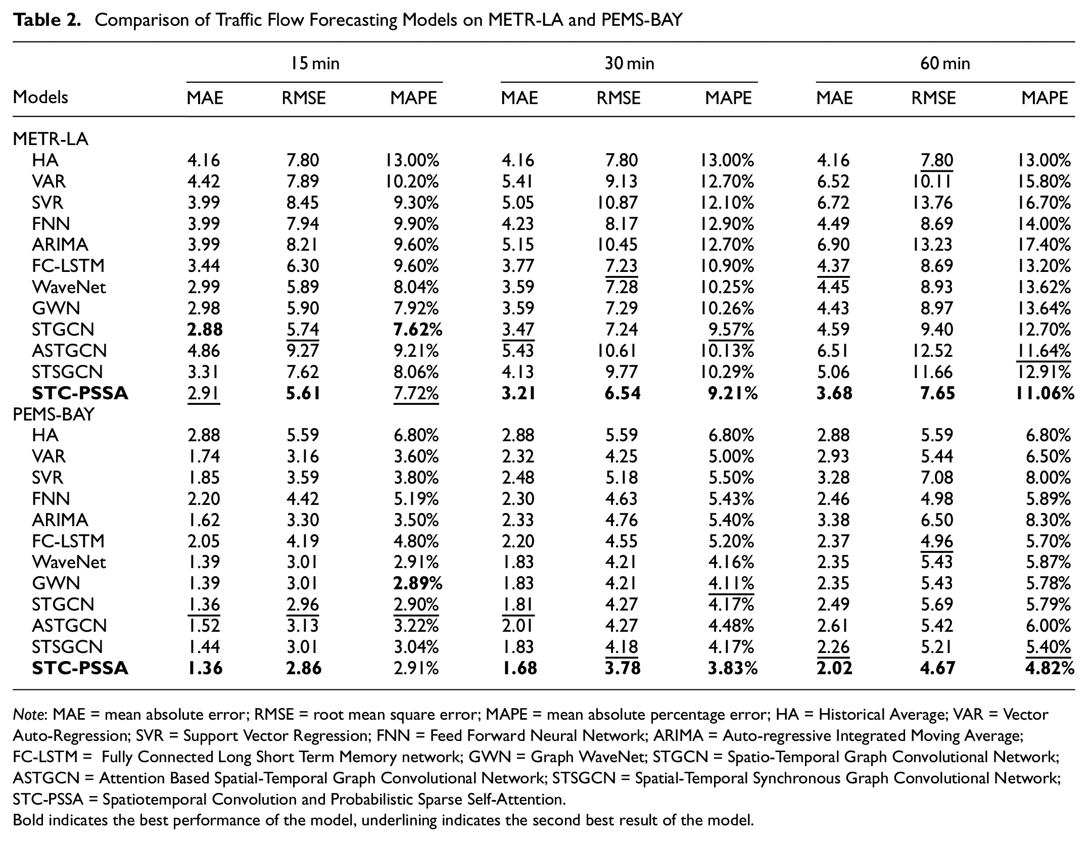
Note: MAE = mean absolute error; RMSE = root mean square error; MAPE = mean absolute percentage error; HA = Historical Average; VAR = Vector Auto-Regression; SVR = Support Vector Regression; FNN = Feed Forward Neural Network; ARIMA = Auto-regressive Integrated Moving Average; FC-LSTM = Fully Connected Long Short Term Memory network; GWN = Graph WaveNet; STGCN = Spatio-Temporal Graph Convolutional Network; ASTGCN = Attention Based Spatial-Temporal Graph Convolutional Network; STSGCN = Spatial-Temporal Synchronous Graph Convolutional Network; STC-PSSA = Spatiotemporal Convolution and Probabilistic Sparse Self-Attention.

Bold indicates the best performance of the model, underlining indicates the second best result of the model.

The formula for calculating the percentage increase summarized in Tables 2 and 3 is as follows:

Table 3.

Predictive Performance of STC-PSSA with Three Variants at Different Times

Models	15 min			30 min			60 min
Models	MAE	RMSE	MAPE	MAE	RMSE	MAPE	MAE	RMSE	MAPE
METR-LA
NG-TCN	2.95	5.72	7.78%	3.29	6.78	9.39%	3.72	7.91	11.88%
FC→G-TCN	3.02	5.87	7.92%	3.45	6.99	9.57%	3.98	8.22	12.17%
NSTC	2.78	5.65	7.66%	3.36	7.00	9.94%	4.20	8.66	11.71%
NPA	2.89	5.63	7.70%	3.40	7.08	10.12%	4.26	8.70	11.96%
NSTC-PA	2.98	5.89	7.98%	3.58	7.29	10.24%	4.43	8.98	13.58%
STC-PSSA	2.91	5.61	7.72%	3.21	6.54	9.21%	3.68	7.65	11.06%
PEMS-BAY
NG-TCN	1.39	2.91	2.95%	1.79	3.92	3.99%	2.25	4.98	5.16%
FC→G-TCN	1.45	2.99	3.01%	1.89	4.17	4.18%	2.35	5.19	5.33%
NSTC	1.40	2.98	2.92%	1.85	4.25	4.26%	2.34	5.37	5.85%
NPA	1.42	3.00	2.98%	1.90	4.26	4.30%	2.30	5.40	5.92%
NSTC-PA	1.43	3.04	3.07%	1.88	4.29	4.42%	2.37	5.46	5.96%
STC-PSSA	1.36	2.86	2.91%	1.68	3.78	3.83%	2.02	4.67	4.82%

Note: STC-PSSA = spatiotemporal convolution and probabilistic sparse self-attention; MAE = mean absolute error; RMSE = root mean square error; MAPE = mean absolute percentage error; NG-TCN = lacks NG-TCN module; FC→G-TCN = lacks G-TCN, and uses a simple fully connected neural network to replace GTCN; NSTC = lacks a spatiotemporal convolutional network module but features a module for a probabilistic sparse self-attention mechanism; NPA = lacks a probabilistic sparse selfattention mechanism module but includes a spatiotemporal convolutional network module; NSTC-PA = lacks a spatiotemporal convolutional network module and a probabilistic sparse self-attention mechanism module.

Bold indicates the best performance of the model, underlining indicates the second best result of the model.

ξ = \frac{α_{\min} - α}{α_{\min}}

(20)

where $α_{\min}$ is the minimum value in the baseline model at the corresponding time and corresponding indicators, and $α$ is the corresponding result value of STC-PSSA.

The STC-PSSA model improves over the state-of-the-art method in MAE, RMSE, and MAPE by 7.5%, 9.5%, 3.8%, and 11.5%, 1.9%, and 5.1% for the 30-min and 60-min forecasting on METR-LA, respectively. Correspondingly, on the data set PEMS-Bay, the improvements are 7.2%, 9.6%, 6.8%, and 10.6%, 5.9%, and 10.7%, respectively. Statistical methods (HA, VAR, ARIMA), as well as traditional machine learning methods (SVR, FC-LSTM), exhibit poor forecasting accuracy as they do not take into account spatial correlation. The spatiotemporal graph convolutional network models, specifically STGCN and STSGCN, effectively manage non-Euclidean traffic data and display superior predictive performance. ASTGCN uses the attention mechanism to efficiently capture the temporal dependence of the sequence with better forecasting. Graph WaveNet incorporates GCN into TCN for improved performance compared with ASTGCN and STG-NCDE. However, Graph WaveNet does not incorporate the self-attention mechanism to further capture hidden spatiotemporal features. In contrast, as can be seen from Table 2, the model evaluation metrics of the STC-PSSA model show good performance in both data sets, for the contrasting values of the model evaluation metrics under different time periods, proving the effectiveness of the STC-PSSA model in capturing the dynamic spatiotemporal characteristics of the traffic flow by embedding the GCN into the TCN and combining it with the spatiotemporal convolution and the probabilistic sparse self-attention mechanism. The construction of an adaptive adjacency matrix and the stacking of GCN spatiotemporal layers with different parameters effectively capture the dynamic associations of hidden nodes in road networks over time. In addition, the STC-PSSA model uses stacked expansive causal convolutional networks and a probabilistic sparse self-attention mechanism to perform effective long-term forecasting. Compared with the baseline model, the STC-PSSA model exhibits the most outstanding predictive performance. Moreover, as the testing time increases, the STC-PSSA model showcases superior training performance, higher predictive accuracy, and excellent long-term forecasting capabilities.

In addition, Figure 6 shows the actual and predicted values of STC-PSSA at the 30th and 60th min at nodes 700 to 1,200 in the PEMS-BAY data set. Obviously, all the models show good prediction accuracy and successfully capture the temporal and spatial characteristics of traffic flow.

Figure 6.

Visualization of traffic prediction on PEMS-BAY data set.

Ablation Experiment

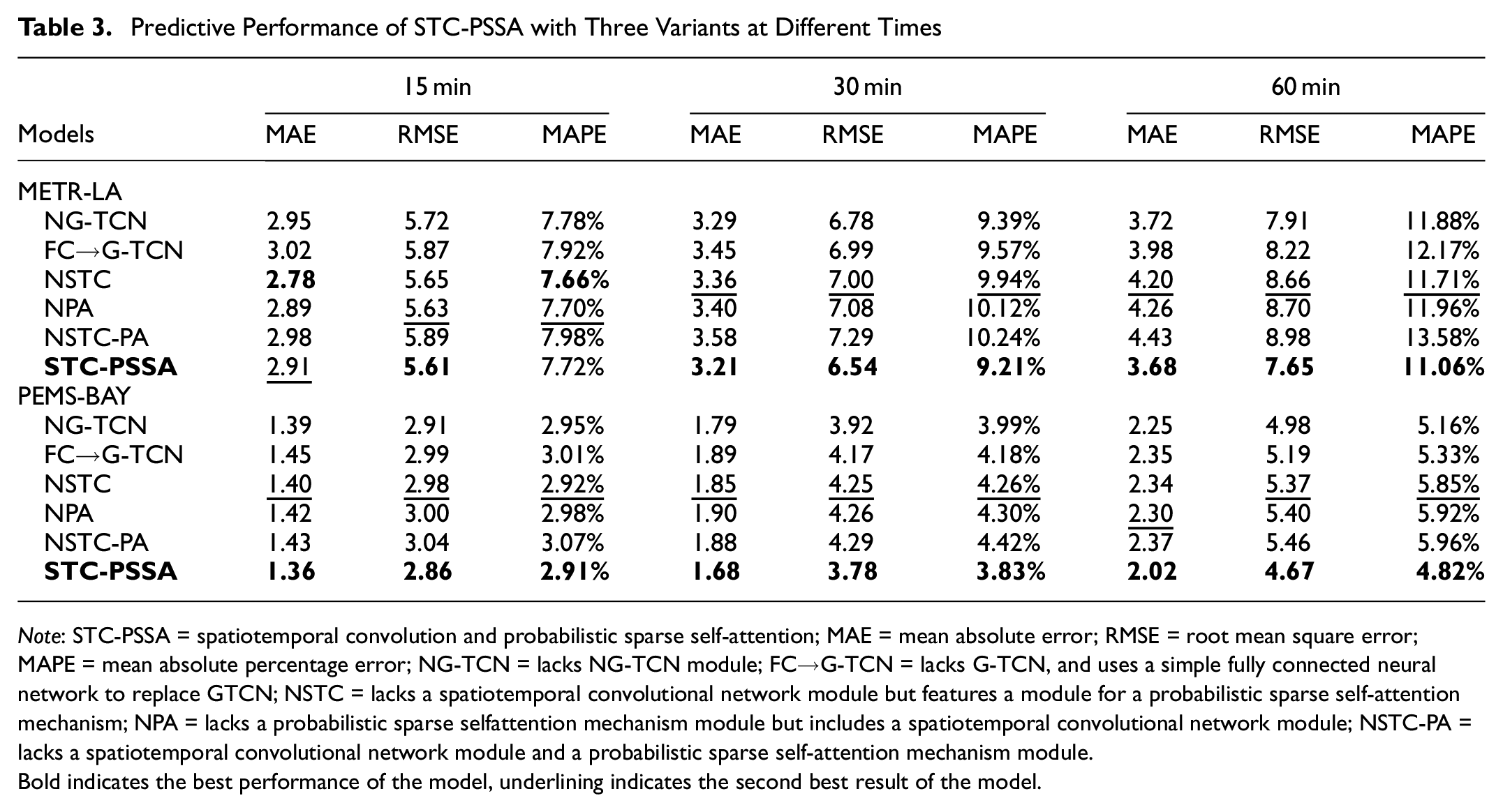
To examine the effectiveness of different modules of the STC-PSSA model, this paper presents three variants of the STC-PSSA model and evaluates the impact of the spatiotemporal convolutional layer and multihead probabilistic sparse self-attention mechanism on model forecasting performance. And the three variants are compared with the STC-PSSA model for 15-min, 30-min, and 60-min traffic flow predictions on the METR-LA and PEMS-BAY data sets, as shown in Table 3.

The distinctions between these five variant models and the STC-PSSA model are as follows:

NG-TCN: This model lacks NG-TCN module.

FC→G-TCN: This model lacks G-TCN, and uses a simple fully connected neural network to replace G-TCN.

NSTC: The model lacks a spatiotemporal convolutional network module but features a module for a probabilistic sparse self-attention mechanism.

NPA: The model lacks a probabilistic sparse self-attention mechanism module but includes a spatiotemporal convolutional network module.

NSTC-PA: The model lacks a spatiotemporal convolutional network module and a probabilistic sparse self-attention mechanism module.

As can be seen from the table, the fully connected neural network can learn the nonlinear relationship of input data, and it cannot effectively capture the time sequence information of input data, because the fully connected layer does not explicitly consider the order and time dependence of input data. In contrast, G-TCN can capture the long-term dependence in time series data by introducing a gating mechanism, and can better model the time series characteristics and relationships in traffic data, thus improving the accuracy of traffic flow prediction. A diffusion graph convolution network can consider a wider range of neighbor nodes by diffusion operation on the graph. In contrast, the traditional graph convolution network usually only considers the information of the directly adjacent nodes. By considering a wider range of neighbor relations, the diffusion graph convolution network can better capture the global structure and interaction between nodes. In addition, when dealing with sparse graphs or graph data containing missing data, the traditional graph convolution network may face challenges. The diffusion graph convolution network can spread information on the graph through diffusion operation, and alleviate the problems caused by sparsity and incomplete data. It can use the information of neighboring nodes to fill the missing values and improve the robustness of the model.

Compared with the NSTC, NPA, and NSTC-PA models, the STC-PSSA model on the PEMS-BAY data set decreased by approximately 2.94%, 4.22%, and 4.90% in 15 min, and the RMSE decreased by approximately 4.20%, 4.67%, and 6.29%, respectively. At 30 min, the MAE decreased by approximately 10.12%, 11.58%, and 11.90%, respectively, and the RMSE decreased by approximately 13.94%, 11.27%, and 13.49%, respectively. At 60 min, the MAE decreased by approximately 15.84%, 12.17%, and 17.33%, respectively, and the RMSE decreased by approximately 14.99%, 13.52%, and 16.92%, respectively. Similarly, the STC-PSSA model achieved excellent forecasting performance on the METR-LA data set. It is thus demonstrated that the PSSA and ST-Conv proposed in this paper can efficiently process long-term sequence data and perform forecasting. At the same time, it is demonstrated that the embedding of GCN into TCN can be efficient in capturing the temporal and spatial correlation of the traffic flow simultaneously and in dealing with the spatial characteristics of various time levels, which makes the forecasting performance of the STC-PSSA model far exceed that of the baseline model. Furthermore, Table 3 demonstrates that the STC-PSSA model exhibits enhanced predictive capabilities for future traffic flow with an increase in training duration.

As shown in Table 4, the calculation time cost of training and reasoning of STC-PSSA and the other three methods on PEMS-BAY data set are shown.

Table 4.

Comparison of Computation Time of Different Models

Models	Computation Time
Models	Training(s/epoch)	Inference(s/epoch)
PEMS-BAY
GWN	189.21	7.85
STGCN	61.80	97.31
STSGCN	1006.54	11.52
STC-PSSA	92.78	6.38

Note: GWN = Graph WaveNet; STGCN = Spatio-Temporal Graph Convolutional Network; STSGCN = Spatial-Temporal Synchronous Graph Convolutional Network; STC-PSSA = Spatiotemporal Convolution and Probabilistic Sparse Self-Attention.

Bold indicates the best performance of the model, underlining indicates the second best result of the model.

The STC-PSSA model designed in this paper is operated by efficient graph convolution and the model is able to handle large-scale traffic prediction tasks effectively. This scalability ensures the applicability of the model in real traffic networks without degrading the performance. Meanwhile the STC-PSSA model incorporates a spatiotemporal graph convolution network and a PSSA mechanism. The combination enables the model to effectively capture spatial dependencies and temporal dynamics in traffic data. Several potential optimization strategies are explored to improve computational efficiency. Small batch training and model parameter optimization are used in the implementation of the STC-PSSA model, aiming to increase the computational speed and reduce the training and inference time. It can be observed that STGCN takes the longest time because of stacking multiple GCNs, while STC-PSSA takes a little longer than STGCN, but its prediction performance is more accurate. In addition, compared with Graph WaveNet (GWN), STC-PSSA has achieved better results in time consumption and prediction accuracy. Through the reasoning of the PEMS-BAY data set, STC-PSSA is the most efficient model, and it takes less time to obtain the highest prediction accuracy.

To visualize the role of the probabilistic sparse self-attention mechanism in STC-PSSA, in this paper, subgraphs containing 10 nodes each from PEMS-BAY are selected and the attention matrices between the nodes are visualized, as shown in Figure 6. In the attention matrix, the first row indicates the correlation strength between each node and the first node. For example, the first row in Figure 7a shows that the traffic flow of the 0th node has the highest degree of correlation with the 5th and 9th because these three nodes are similar in the real road network, as shown in Figure 7b. Therefore, the model in this paper not only has the best prediction performance, but also has the advantage of interpretability.

Figure 7.

The attention matrix between nodes is visualized: (a) the attention matrix obtained by the probabilistic sparse attention mechanism on PEMS-BAY; and (b) approximate position of the 10 nodes on the real road network.

To provide a clearer understanding of the STC-PSSA model, this paper presents visualizations of its experimental results, using FNN, FC-LSTM, Graph WaveNet, and STGCN on the PEMS-BAY data set, as depicted in Figure 8. It is evident from the three figures that the STC-PSSA model outperforms the FNN, FC-LSTM, Graph WaveNet, and STGCN models in predicting traffic flow. This suggests that the model is better at capturing the dynamic spatiotemporal features of traffic flow. Meanwhile, as the forecasting duration increases, the increase in forecasting error becomes smaller. When the forecasting duration exceeds 15 min, the forecasting errors of STC-PSSA are significantly smaller than other models compared. This indicates that the forecasting performance of the STC-PSSA model is superior for long-range forecasting.

Figure 8.

Visual comparison of different errors. The prediction step indicates time step or prediction step. This represents the interval at which the forecasting model predicts the traffic flow in each time step: (a) MAE results visualization; (b) MAPE results visualization; and (c) RMSE results visualization.

To sum up, the STC-PSSA model provides the best prediction results at different time intervals. The STC-PSSA model can accurately predict traffic flow and capture the temporal and spatial characteristics of traffic flow. This demonstrates the excellent predictive abilities of the STC-PSSA model for traffic flow and its efficacy in traffic forecasting.

Conclusion

This paper presents an effective and accurate traffic forecasting model, STC-PSSA, which not only accounts for the non-Euclidean structure of the traffic network but also properly captures the dynamic spatiotemporal features of the traffic flow, thereby overcoming the problems of insufficient spatiotemporal capture by previous models and the difficulty of dealing with long time series. The STC-PSSA model incorporates the strengths of TCN, GCN, and the probabilistic sparse self-attention mechanism. It captures the intricate time characteristics of traffic flow using G-TCN, followed by capturing the dynamic spatial correlation of traffic flow using an adaptive adjacency matrix based on GCN. It then thoroughly leverages the dynamic spatial and temporal characteristics of traffic flow using the probabilistic sparse self-attention mechanism, which ultimately enhances the precision of traffic flow forecasting. Experiments demonstrate that the STC-PSSA model can capture the dynamic spatiotemporal characteristics of traffic flow effectively and simultaneously, as well as process long-term sequence data efficiently, and the forecasting performance is significantly better than that of the baseline model. As the duration of training increases, the STC-PSSA model exhibits better training performance, which leads to higher accuracy in traffic flow forecasting and better medium- and long-term traffic flow forecasting.

In reality, a variety of external factors, such as the weather and current social events, have an impact on traffic flow forecasting. Future research will take outside factors into account to boost the model’s training efficiency and predicting precision. In addition, the expansion of the STC-PSSA model to large data sets will be further investigated to improve the forecasting time efficiency as well as the forecasting accuracy.

Footnotes

Author Contributions

The authors confirm contribution to the paper as follows: study conception and design: Linbiao Chen; data collection: Xijun Zhang; analysis and interpretation of results: Jie Cao; draft manuscript preparation: Linbiao Chen and Hong Zhang. All authors reviewed the results and approved the final version of the manuscript.

Declaration of Conflicting Interests

The author(s) declared no potential conflicts of interest with respect to the research, authorship, and/or publication of this article.

Funding

The author(s) disclosed receipt of the following financial support for the research, authorship, and/or publication of this article: This work is supported by the Key R&D Program of Gansu Province (23YFGA0063); the National Natural Science Foundation of China (62363022,61663021); the Natural Science Foundation of Gansu Province (22JR5RA226, 23JRRA886); and the Gansu Provincial Department of Education: Industrial Support Plan Project (2023CYZC-35).

ORCID iD

Linbiao Chen

References

Zhong

Cui

Wang

Forecasting Transportation Network Speed Using Deep Capsule Networks with Nested LSTM Models. IEEE Transactions on Intelligent Transportation Systems, Vol. 22, No. 8, 2021, pp. 4813–4824.

Hong

Chen

Zhu

Temporal Multi-Graph Convolutional Network for Traffic Flow Forecasting. IEEE Transactions on Intelligent Transportation Systems, Vol. 22, No. 6, 2021, pp. 3337–3348.

Zhao

Song

Zhang

Liu

Wang

Lin

Deng

T-GCN: A Temporal Graph Convolutional Network for Traffic Forecasting. IEEE Transactions on Intelligent Transportation Systems, Vol. 21, No. 9, 2020, pp. 3848–3858.

Guo

Lin

Feng

Song

Wan

Attention Based Spatiotemporal Graph Convolutional Networks for Traffic Flow Forecasting. Proceedings of the AAAI Conference on Artificial Intelligence, Vol. 33, No. 1, 2019, pp. 922–929.

Yin

Zhu

Spatial-Temporal Graph Convolutional Networks: A Deep Learning Framework for Traffic Forecasting. Proceedings of the AAAI Conference on Artificial Intelligence, 2018, pp. 3634–3640.

Song

Lin

Guo

Wan

Spatial-Temporal Synchronous Graph Convolutional Networks: A New Framework for Spatiotemporal Network Data Forecasting. Proceedings of the AAAI Conference on Artificial Intelligence, Vol. 34, No. 1, 2020, pp. 914–921.

Dai

Liu

Gao

Lin

G.-J.

Xiong

Spatial-Temporal Transformer Networks for Traffic Flow Forecasting. arXiv Preprint arXiv:2001.02908, 2020.

Lippi

Bertini

Frasconi

Short-Term Traffic Flow Forecasting: An Experimental Comparison of Time-Series Analysis and Supervised Learning. IEEE Transactions on Intelligent Transportation Systems, Vol. 14, No. 2, 2013, pp. 871–882.

Shekhar

Williams

B. M.

Adaptive Seasonal Time Series Models for Forecasting Short-Term Traffic Flow. Transportation Research Record: Journal of the Transportation Research Board, 2008. 2024: 116–125.

10.

Deng

Shahabi

Demiryurek

Zhu

Liu

Latent Space Model for Road Networks to Predict Time-Varying Traffic. Proc., KDD, San Francisco, CA, 2018.

11.

Niepert

Ahmed

Kutzkov

Learning Convolutional Neural Networks for Graphs. International Conference on Machine Learning, Vol. 48, 2016, pp. 2014–2023.

12.

Cui

Zheng

Spatio-Temporal Graph Convolution for Skeleton Based Action Recognition. Proceedings of the AAAI Conference on Artificial Intelligence, Vol. 32, 2018, pp. 3482–3489.

13.

Bruna

Zaremba

Szlam

LeCun

. Spectral Networks and Locally Connected Networks on Graphs. Proc., International Conference on Learning Representations. Banff, Canada, 2014.

14.

Zhu

Tsui

K.-L.

Multi-Graph Convolutional-Recurrent Neural Network (MGC-RNN) for Short-Term Forecasting of Transit Passenger Flow. IEEE Transactions on Intelligent Transportation Systems, Vol. 23, No. 10, 2022, pp. 18155–18174.

15.

Bogaerts

Masegosa

A. D.

Angarita-Zapata

J. S.

Onieva

Hellinckx

A Graph CNN-LSTM Neural Network for Short and Long-Term Traffic Forecasting Based on Trajectory Data. Transportation Research Part C: Emerging Technologies, Vol. 112, 2020, pp. 62–77.

16.

Lasenby

Spatiotemporal Attention-Based Graph Convolution Network for Segment-Level Traffic Prediction. IEEE Transactions on Intelligent Transportation Systems, Vol. 23, No. 7, 2022, pp. 8337–8345.

17.

Zhang

Guo

Zhao

Zheng

Chen

A Graph-Based Temporal Attention Framework for Multi-Sensor Traffic Flow Forecasting. IEEE Transactions on Intelligent Transportation Systems, Vol. 23, No. 7, 2022, pp. 7743–7758.

18.

Zheng

Chai

W. K.

Katos

A Dynamic Spatiotemporal Deep Learning Framework for Traffic Speed Forecasting on Large-Scale Road Networks. Expert Systems with Applications, Vol. 195, 2022, p. 116585.

19.

Wen

Wang

RPConvformer: A Novel Transformer-Based Deep Neural Networks for Traffic Flow Prediction. Expert Systems with Applications, Vol. 218, 2023, p. 119587.

20.

Bui

Nguyen

Dynamic Spatial Transformer WaveNet Network for Traffic Forecasting. Vietnam Journal of Computer Science, Vol. 10, 2022, pp. 25–38.

21.

Chen

Shi

Traffic Flow Prediction Using Multi-View Graph Convolution and Masked Attention Mechanism. Computer Communications, Vol. 194, 2022, pp. 446–457.

22.

Zhou

Zhang

Peng

Zhang

Xiong

Zhang

Informer: Beyond Efficient Transformer for Long Sequence Time-Series Forecasting. arXiv Preprint arXiv:2012.07436, 2020.

23.

Huang

Dou

Luo

Wang

Zhou

Adaptive Spatiotemporal Transformer Graph Network for Traffic Flow Forecasting by IoT Loop Detectors. IEEE Internet of Things Journal, Vol. 10, No. 2, 2023, pp. 1642–1653.

24.

Chen

Xue

ADGCN: An Asynchronous Dilation Graph Convolutional Network for Traffic Flow Forecasting. IEEE Internet of Things Journal, Vol. 9, No. 5, 2022, pp. 4001–4014.

25.

Zhou

Yang

Zhang

Trajcevski

Zhong

Khokhar

Reinforced Spatiotemporal Attentive Graph Neural Networks for Traffic Forecasting. IEEE Internet of Things Journal, Vol. 7, No. 7, 2020, pp. 6414–6428.

26.

Zhao

Liu

Sun

Jia

Zhang

Attention-Based Dynamic Spatiotemporal Graph Convolutional Networks for Traffic Speed Forecasting. Expert Systems with Applications, Vol. 204, 2022, p. 117511.

27.

Wang

Chen

Zhou

Zhang

Zou

An Improved WaveNet Network for Multi-Step-Ahead Wind Energy Forecasting. Energy Conversion and Management, Vol. 278, 2022, p. 116709.

28.

Zhang

Spatiotemporal Residual Graph Attention Network for Traffic Flow Forecasting. IEEE Internet of Things Journal, Vol. 10, No. 13, 2023, pp. 11518–11532.