Experimental Research and Application of Small-Strain Soil Hardening Model Parameters in a Major Project in Hangzhou

Abstract

According to current research, the small-strain soil hardening model (HSS model) is being used more and more widely because it can consider the small-strain characteristics of soil, making the corresponding numerical analysis results more accurate. At present, research into the test value of HSS model parameters of soil mass is mainly concentrated in Shanghai. Given the limits of the test conditions, there has been notably insufficient research into the value of small-strain parameters. Considering the regional differences of soil parameters, this paper, based on an actual project, conducts the HSS model parameter test value study on the main soil layers in the west of Hangzhou, focusing on the value study of small-strain parameters. The corresponding results are used for numerical analysis. The research shows that, compared with the Mohr–Coulomb model, the numerical analysis results using the HSS model are obviously closer to the measured data, and the prediction of the lateral deformation and its change law of the diaphragm wall is obviously more accurate. At the same time, when other HSS model parameters are unchanged, the numerical results using in situ small-strain parameters are closer to the measured results than using indoor small-strain parameters, and the corresponding deformation prediction accuracy is higher. The research results provide valuable references for determining HSS model parameters and engineering applications in the western area of Hangzhou.

Keywords

HS-Small model small strain parameter numerical analysis indoor soil test field wave velocity test

The small-strain soil hardening model (HSS model) is developed to capture the small-strain behavior of soils, which is crucial for predicting soil deformation in underground engineering projects. The numerical analysis using the HSS model produces more accurate deformation predictions compared with the Mohr–Coulomb model (M-C model), the Modified Cambridge model (MCC model), and the soil hardening model (HS model) ( 1 – 5 ). However, given the large number of parameters involved in the HSS model and the high requirements of test conditions, it is difficult to obtain values of all parameters through tests. Besides, the existing studies into HSS model parameters mainly concentrated in Shanghai in China, and the research results in other regions are relatively rare ( 6 – 10 ).

This study presents the numerical analysis of the excavation of the foundation pit project in Hangzhou based on the HSS model. Firstly, the experimental values of HSS model parameters of main soil layers in the western area of Hangzhou are studied and used for numerical analysis. Secondly, the deformation predicted by the HSS model is compared with the M-C model. Finally, the reference initial shear modulus obtained by indoor resonant column tests (indoor G^ref₀) and in situ wave velocity testing (in situ G^ref₀) are compared. The research results provide valuable references for determining HSS model parameters and engineering applications in the western area of Hangzhou.

Project Description

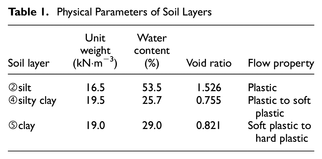
The foundation pit for this project is situated in the future science and technology city section of Yuhang District, Hangzhou. The surrounding area is currently undeveloped. The foundation pit is rectangular and approximately 100.1 m in length and 28.0 m in width. It is divided into two sections, the south and the north. The excavation depth of the south block is 23.95 m, while that of the north block is 38.3 m. This is the deepest excavation depth among public construction facilities in Zhejiang Province. The design leveling elevation for the project site is −3.00 m. Figure 1 and Table 1 provide relevant dimensions, elevations, stratum distribution, and physical property parameters of the soil. The site has more than 10 m of silt (layer ②) beneath the superficial surface, which significantly affects the deformation of the foundation pit. Below the silt soil layer, there are mainly a silty clay layer (layer ④), a clay layer (layer ⑤), and a gravel layer (layer ⑤). In addition, there is a strongly weathered argillaceous siltstone layer (layer ⑩₂) and moderately weathered argillaceous siltstone layer (layer ⑩₃). The silty clay and clay layers continue to exert influence on the deformation of the foundation pit.

Figure 1.

Outline of foundation pit.

Table 1.

Physical Parameters of Soil Layers

Soil layer	Unit weight (kN·m⁻³)	Water content (%)	Void ratio	Flow property
②silt	16.5	53.5	1.526	Plastic
④silty clay	19.5	25.7	0.755	Plastic to soft plastic
⑤clay	19.0	29.0	0.821	Soft plastic to hard plastic

The foundation pit is constructed using an “underground diaphragm wall + support + water-stop curtain” enclosure structure. The underground diaphragm wall in the southern area is 1.0 m in thickness and 40 m in height, while the thickness and height of the wall in the northern area are 1.2 m and 46.3 m, respectively. Both walls are constructed using C35 concrete. There are five supports in the southern block and eight supports in the northern block, which are made of reinforced concrete. The first support section is 0.9-m wide and 0.8-m high, while the second and third sections are 1.1-m wide and 0.9-m high. The fourth to eighth support sections are 1.2-m wide and 1.1-m high. The groove wall of the underground diaphragm wall is reinforced by φ850@600 triaxial cement mixing piles on both sides. The triaxial cement mixing piles also serve as a water-stop curtain. The joints of the underground diaphragm wall are reinforced for waterproofing using RJP double high-pressure jet grouting piles with a diameter of 2.0 m.

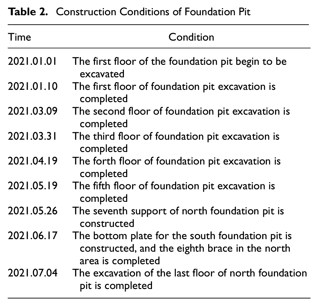
The excavation of a foundation pit typically follows the principle of “layering, division, and symmetry” which involves dividing the excavation process into manageable layers and ensuring that the excavation is symmetrical to prevent instability. More details of the excavation sequence are summarized in Table 2. In addition to the construction process, the lateral deformation of the underground diaphragm wall must be monitored to ensure stability. Figure 1 shows the layout of the monitoring points for this purpose.

Table 2.

Construction Conditions of Foundation Pit

Time	Condition
2021.01.01	The first floor of the foundation pit begin to be excavated
2021.01.10	The first floor of foundation pit excavation is completed
2021.03.09	The second floor of foundation pit excavation is completed
2021.03.31	The third floor of foundation pit excavation is completed
2021.04.19	The forth floor of foundation pit excavation is completed
2021.05.19	The fifth floor of foundation pit excavation is completed
2021.05.26	The seventh support of north foundation pit is constructed
2021.06.17	The bottom plate for the south foundation pit is constructed, and the eighth brace in the north area is completed
2021.07.04	The excavation of the last floor of north foundation pit is completed

Parameters of the HSS Model

The HSS model consists of 13 parameters, including 11 HS model parameters and two small-strain parameters that overcome the limitations of the HS model. The HSS model can, therefore, simulate the variation of soil stiffness in the small-strain region (<10⁻³). The description of the constitutive relationship of the HSS model can be found in Benz ( 11 ). The physical meaning of each parameter and the method of laboratory tests are shown in Table 3. The values of the parameters ψ, K₀, m, and ν_ur are obtained from the existing studies ( 13 – 17 ). The other parameters are obtained by the standard consolidation test, the triaxial consolidation drainage shear test, the triaxial consolidation drainage load-unload shear test, and the resonance column test. The instrumentation and equipment requirements and the main operational process of each test are referenced to Liang et al. ( 7 ) and are conducted in accordance with the Standard of Geotechnical Test Methods (GB/T 50123-2019). The HSS model parameters for the primary soil layers, including silt, silty clay, and clay layers, which have a significant impact on the deformation of the foundation pit during the excavation, are studied. The experimental results obtained are as follows.

Table 3.

Description and Evaluation Method of HSS Model Parameters ( 12 )

Parameters	Unit	Description	Evaluation method
Strength parameters
c′	kPa	Effective cohesion	Triaxial CU or CD test
φ′	(°)	Effective internal friction angle	Triaxial CU or CD test
ψ	(°)	Dilatancy angle	For sand, φ′ > 30°, ψ = (φ′-30), φ′ < 30°, ψ = 0 ( 13 ); for clay, ψ = 0 ( 14 )
R_f	-	Failure ratio	Triaxial CD test
Stiffness parameters
p^ref	kPa	Confining pressure	100 kPa ( 14 )
E^ref_oed	MPa	Reference tangent modulus	Standard consolidation test
E^ref₅₀	MPa	Reference secant modulus when shear stress is 50% of shear strength	Triaxial CD test
E^ref_ur	MPa	Reference unloading–reloading secant modulus	Triaxial CD unloading–reloading test
ν_ur	na	Unloading–reloading Poisson’s ratio	0.2 ( 14 )
K₀	na	Coefficient of normal consolidation static lateral pressure	(1- sinφ) ( 15 )
m	na	Exponential power	For sand and silt, m = 0.5 ( 16 ); for clay, m = 0.5-1 ( 17 )
Small-strain parameter
G^ref₀	MPa	Reference initial shear modulus	Bending element test or small-strain triaxial test or resonant column test
γ_0.7	na	Reference shear strain at which shear modulus is 70% of G^ref₀	Small-strain triaxial test or resonant column test

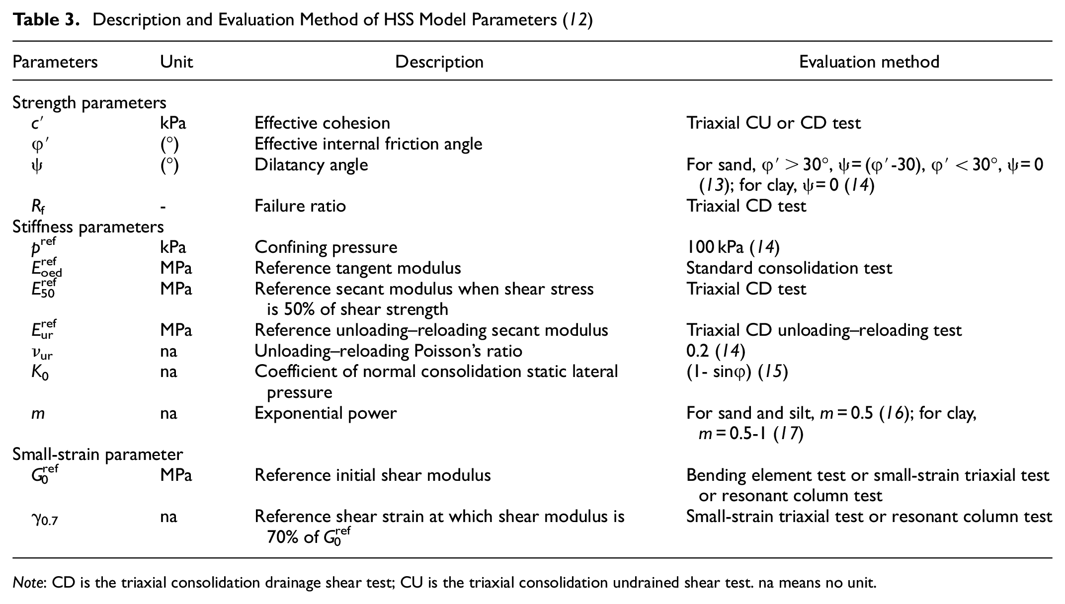
Note: CD is the triaxial consolidation drainage shear test; CU is the triaxial consolidation undrained shear test. na means no unit.

Standard Consolidation Test

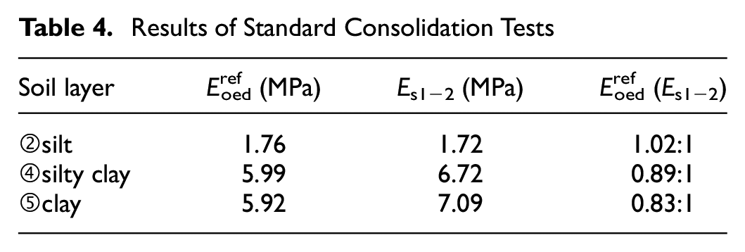
Figure 2a shows the relationship between the vertical load σ_v and the vertical strain ε_v of each soil layer. A quadratic polynomial is used to fit the data points, and the origin is specified for each curve. By substituting the vertical strain value ε_v corresponding to σ_v = 100 kPa into the fitting relationship curve, the reference tangent modulus E^ref_oed under the reference stress (100 kPa) is calculated. The values of E^ref_oed for each soil layer are listed in Table 4.

Table 4.

Results of Standard Consolidation Tests

Soil layer	E ^ref _oed (MPa)	E _s1−2 (MPa)	E ^ref _oed (E_s1−2)
②silt	1.76	1.72	1.02:1
④silty clay	5.99	6.72	0.89:1
⑤clay	5.92	7.09	0.83:1

Figure 2.

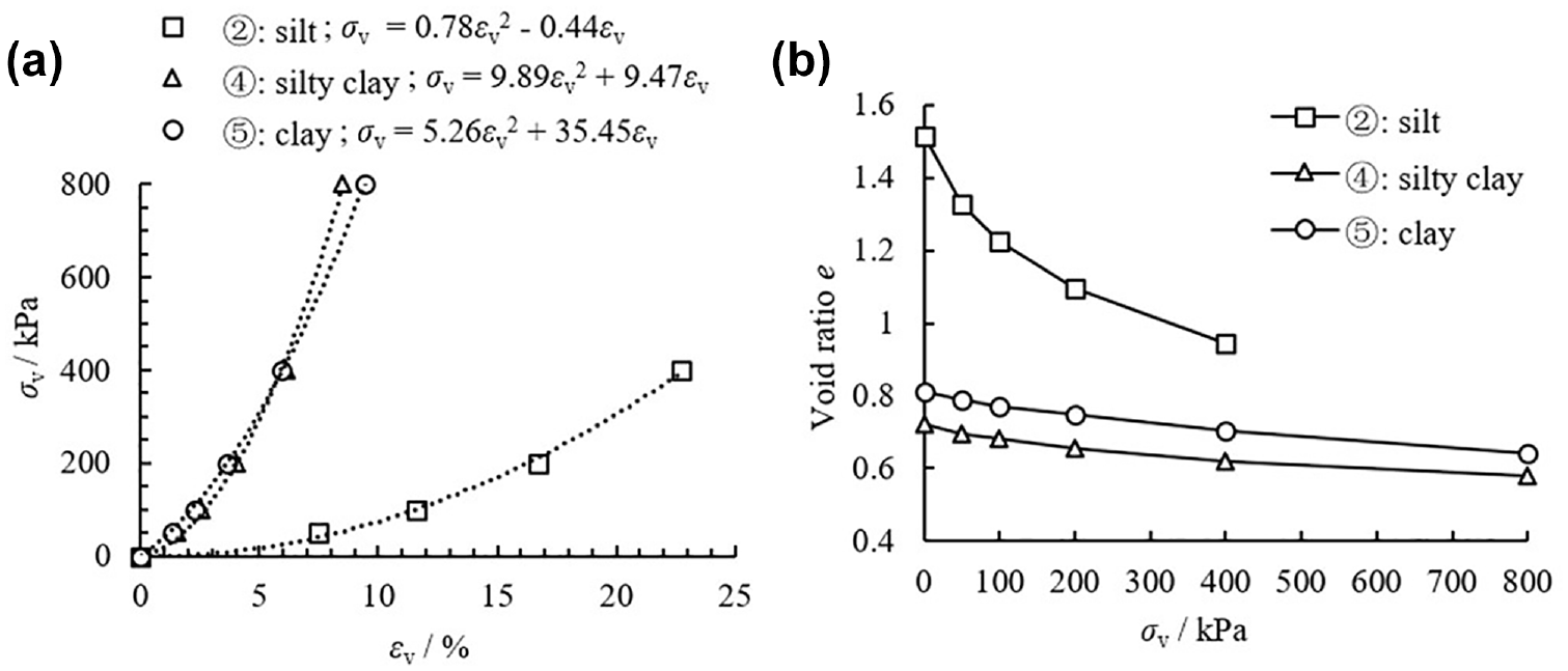
Result curves of standard consolidation tests: (a) relationship between σ_v and ε_v; and (b) relationship between e and σ_v.

Figure 2b shows the relationship between the vertical load σ_v and the void ratio e of each soil layer. The compressive modulus E_s1−2 of each soil layer is obtained based on this curve, which is listed in Table 4. The ratio relationship between E^ref_oed and E_s1−2 of each soil layer is also shown in Table 4, with ratios ranging from approximately 0.83 to 1.02.

Triaxial Consolidation Drainage Shear Test

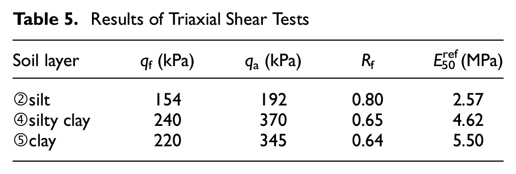
Figure 3 displays the stress–strain relationship for each soil layer under the reference stress obtained from the triaxial consolidation drainage shear test. The q_f and E^ref₅₀ of each soil layer under the reference stresses are listed in Table 5. For the strain softening curves, the peak value is taken as the failure value q_f, while the deviatoric stress value corresponding to 15% axial strain is used as the failure value for other curves. E^ref₅₀ is the secant modulus corresponding to 50% of the ultimate load (i.e., 0.5 q_f), and its value is equal to the slope of the line connecting the origin and the point on the curve corresponding to 0.5 q_f.

Figure 3.

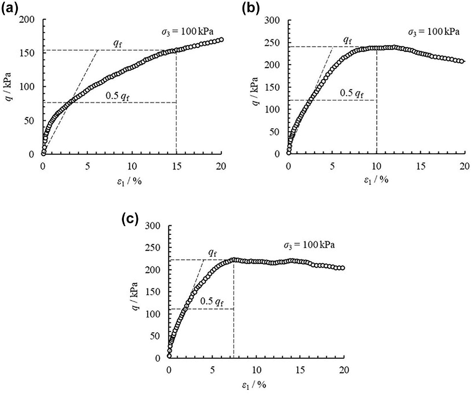
Strain-stress curves of triaxial shear tests: (a) ② silt; (b) ④ silty clay; and (c) ⑤ clay.

Table 5.

Results of Triaxial Shear Tests

Soil layer	q _f (kPa)	q _a (kPa)	R _f	E ^ref ₅₀ (MPa)
②silt	154	192	0.80	2.57
④silty clay	240	370	0.65	4.62
⑤clay	220	345	0.64	5.50

According to the definition of the HSS model, the relationship between the deviatoric stress q and the axial strain ε₁ can be represented by a hyperbolic function, as shown in Equation 1.

\begin{matrix} ε_{1} = \frac{1}{2 E_{50}} \cdot \frac{q}{1 - q / q_{a}} & (q < q_{f}) \end{matrix}

(1)

The linear relationship between $ε_{1} / q$ and $ε_{1}$ can be obtained:

\begin{matrix} \frac{ε_{1}}{q} = \frac{ε_{1}}{q_{a}} + \frac{1}{2 E_{50}} & (q < q_{f}) \end{matrix}

(2)

However, Equations 1 and 2 are theoretically assumed relationships, and the actual stress–strain (q-ε1) curve cannot perfectly match the hyperbolic relationship, especially in the initial stage of the curve (when ε1 is close to 0) and after reaching the peak value. Therefore, when converting the stress–strain relationship curve in Figure 3 to the ε₁/q-ε₁ relationship curve in Figure 4, data points with better linearity are selected for fitting. Data between ε₁ = 1% and the axial strain range corresponding to the failure value q_f are chosen for linear fitting. From Equation 2, it can be observed that the slope of the fitted line in Figure 4 is 1/q_a, where the asymptotic value q_a is the reciprocal of the slope of the fitted line. The failure ratio R_f is defined as the ratio of the failure value q_f to the asymptotic value q_a, and its values are listed in Table 5.

Figure 4.

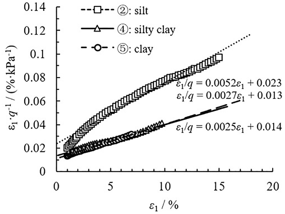
ε ₁/q-ε₁ curves.

Figure 5 gives triaxial consolidation drainage test results for three different confining pressures (50, 100, and 200 kPa) of the ②silt layer. These results are analyzed using the p-q relationship, where p = 1/2 (σ₁ + σ₃) and q = 1/2 (σ₁ − σ₃). The effective cohesion c′ and effective internal friction angle φ′ of the silt soil layer are determined to be 10.1 kPa and 24.0°, respectively. Similarly, for the ④silty clay layer, the c′ and φ′ are found to be 11.2 kPa and 29.9°, respectively. Finally, for the ⑤clay layer, the c′ and φ′ are determined to be 28.7 kPa and 25.9°, respectively.

Figure 5.

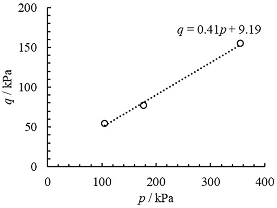
The p-q curve of silt layer.

Triaxial Consolidation Drainage Loading–Unloading Shear Test

Figure 6 shows the stress–strain relationship for each soil layer under the reference stress, as obtained from the triaxial consolidation drainage loading–unloading shear test. It can be inferred that E^ref_ur of the ②silt layer, ④silty clay layer, and ⑤clay layer under the reference stress are 11.6 MPa, 31.3 MPa, and 28.1 MPa, respectively.

Figure 6.

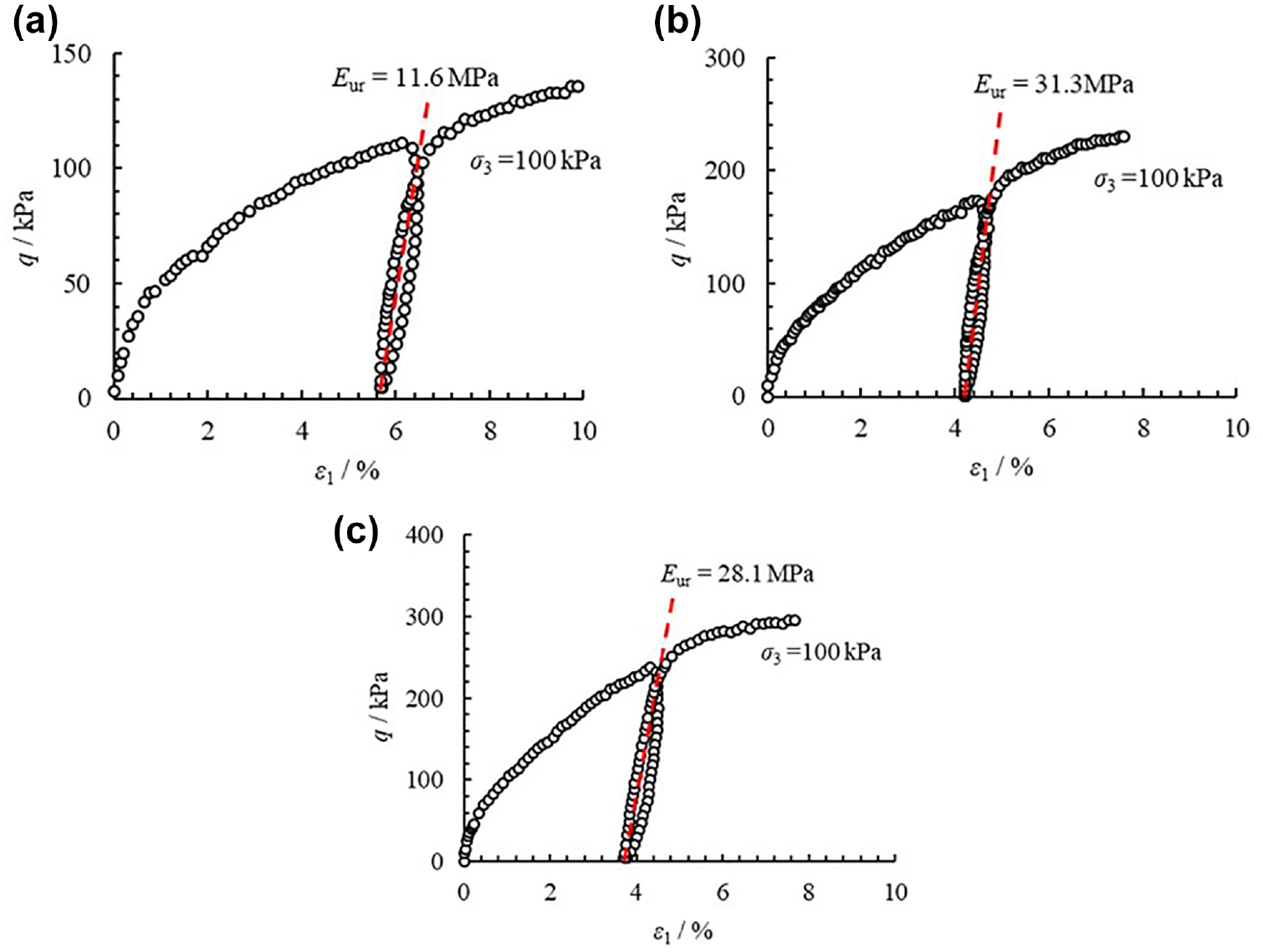
Strain-stress curves of triaxial loading–unloading–reloading tests: (a) ②silt; (b) ④silty clay; and (c) ⑤clay.

Resonant Column Test

Figure 7a shows the correlation between the dynamic shear modulus and the shear strain for each soil layer under the reference stress. Figure 7b displays the curve of the 1/G-γ relationship fitted using the Hardin formula (Equation 3). When γ = 0, the corresponding G represents the small-strain initial shear modulus (G₀), which can be calculated using Equation 4. Besides, the data presented in Figure 7b are obtained under the reference stress. G₀, calculated using Equation 4, represents the small-strain initial shear modulus G^ref₀. The G^ref₀ values for the ②silt layer, ④silty clay layer, and ⑤clay layer are 29.33 MPa, 34.36 MPa, and 33.44 MPa, respectively.

1 / G = a + b γ

(3)

where

G is the dynamic shear modulus of soil,

γ is shear strain,

a and b are constants which can be determined by regression statistical analysis based on test data.

G_{0} = 1 / a

(4)

where G₀ is the initial dynamic shear modulus of the soil.

Figure 7.

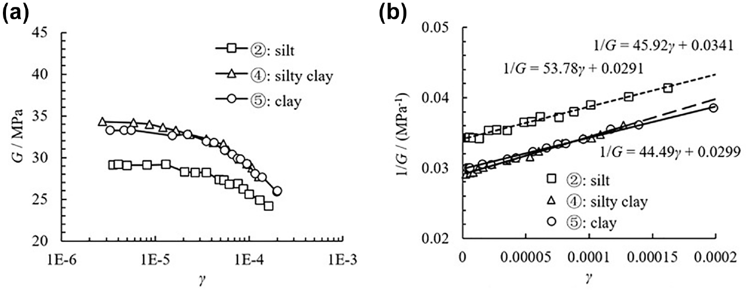
Curves of dynamic shear modulus and strain: (a) relationship between G and γ; and (b) relationship between 1/G and γ.

Figure 8 shows the normalized shear modulus attenuation curves for each soil layer under the reference stress. Specifically, the G/G₀-γ relationship curves of different soil layers are fitted using the DaVidenkoV model. The mathematical function of the DaVidenkoV model is:

G = G_{0} [1 - H (γ)]

(5)

where H(γ) is defined as:

H (γ) = {[\frac{(γ / γ_{0})^{2 B}}{1 + (γ / γ_{0})^{2 B}}]}^{A}

(6)

where A, B, and γ₀ are fitting parameters.

Figure 8.

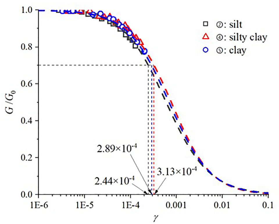
Normalized shear modulus reduction curve.

According to the DaVidenkoV model, the relationship between the normalized shear modulus (G/G₀) and shear strain amplitude (γ) can be plotted within the range of 10⁻⁶ to 10⁻¹. The corresponding shear strain amplitude at which the normalized shear modulus is 0.7 is denoted as γ_0.7. Based on the information provided in the Figure 8, the values of γ_0.7 for the ②silt layer, ④silty clay layer, and ⑤clay layer are 2.44 × 10⁻⁴, 3.13 × 10⁻⁴, and 2.89 × 10⁻⁴, respectively.

Summary of HSS Model Parameters

Table 6 presents the HSS model parameters for the ②silt layer, ④silty clay layer, and ⑤clay layer that are relevant to the project discussed in this paper. The values of m, ν_ur, and K₀ are determined using the empirical method based on Liang et al. ( 7 ). The proportional relationship between the reference modulus is shown in Table 7. All values fall within the statistical range reported by Luo et al. ( 12 ). However, some of the ratios are near the statistical boundary, with a slight deviation from the average value. This result indicates that the test results are reasonably reliable and effectively capture the regional differences in soil layer parameters. In addition, Tables 6 and 7 demonstrate that soil properties in the same region exhibit certain discrepancies.

Table 6.

Summary of HSS Model Parameters

Soil layer	c′/kPa	φ′ (°)	E ^ref _oed (MPa)	E ^ref ₅₀ (MPa)	E ^ref _ur (MPa)	R _f	G ^ref ₀(MPa)		γ _0.7/10⁻⁴	m	ν _ur	K ₀
Soil layer	c′/kPa	φ′ (°)	E ^ref _oed (MPa)	E ^ref ₅₀ (MPa)	E ^ref _ur (MPa)	R _f	Indoor	In-situ	γ _0.7/10⁻⁴	m	ν _ur	K ₀
②silt	10.1	24.0	1.76	2.57	11.6	0.80	29.33	48.01	2.44	0.5	0.2	0.59
④silty clay	11.2	29.9	5.99	4.62	31.3	0.65	34.36	69.12	3.13	0.5	0.2	0.50
⑤clay	28.7	25.9	5.92	5.50	28.1	0.64	33.44	55.17	2.89	0.5	0.2	0.56

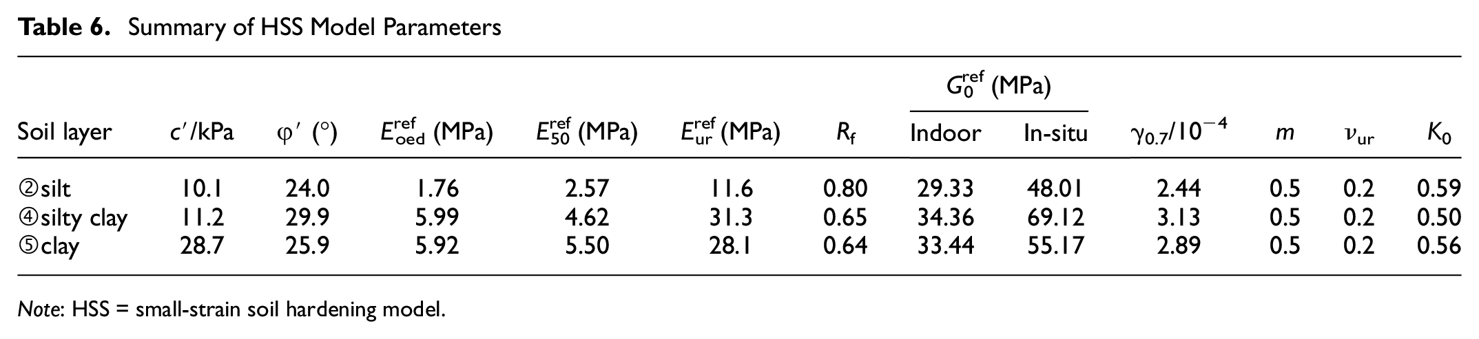
Note: HSS = small-strain soil hardening model.

Table 7.

Proportional Relation of Reference Modulus

Soil layer	E ^ref _oed/E_s1−2	E ^ref ₅₀/E^ref_oed	E ^ref _ur/E^ref_oed	G ^ref ₀/E^ref_ur
②silt	1.02	1.46	6.59	2.53
④silty clay	0.89	0.77	5.23	1.10
⑤clay	0.83	0.93	4.74	1.19

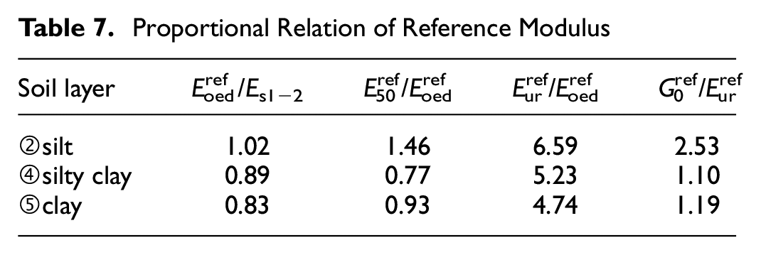
Table 6 also shows the in situ G^ref₀ value converted from the in situ cross-hole wave velocity test. The conversion formula is as follows:

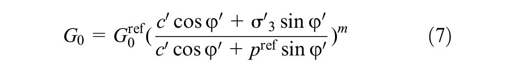
G_{0} = G_{0}^{ref} (\frac{c' \cos φ' + {σ'}_{3} \sin φ'}{c' \cos φ' + p^{ref} \sin φ'})^{m}

(7)

where G₀ is the initial shear modulus obtained from the field wave velocity test.

Numerical Simulation

A three-dimensional numerical model is established using Plaxis 3-D to analyze the lateral deformation of diaphragm wall during foundation pit excavation. The model size is set to 350 m × 280 m × 120 m (length × width × height). The distance between the model boundary and the edge of the foundation pit is more than three times the maximum excavation depth. Additionally, the distance between the model bottom and the bottom of the pit is more than twice the maximum excavation depth. The dimension of the model does not affect the results of the excavation of the foundation pit in this case ( 18 ). The bottom of the model is set as a fixed impermeable boundary, and the surrounding and surface are set as permeable boundaries. The underground diaphragm wall is simulated using solid elements, while reinforced concrete supports are simulated using beam elements. Engineering piles at the bottom of the foundation pit in the south area are simulated using “embedded piles” within the beam elements. The mesh division accuracy of the model is classified as “medium,” and the densification coefficients of the soil in the foundation pit and the enclosure structure are set to 0.25 and 0.25, respectively, forming a total of 119,695 units. According to the geotechnical engineering investigation report and the foundation pit drainage plan, the groundwater level is set at −2 m, and the water level in the foundation pit drops to 0.5 m below the bottom of the foundation pit. The simulated excavation process is the same as the actual construction process (Table 2), and the excavation sequence is subdivision and block excavation.

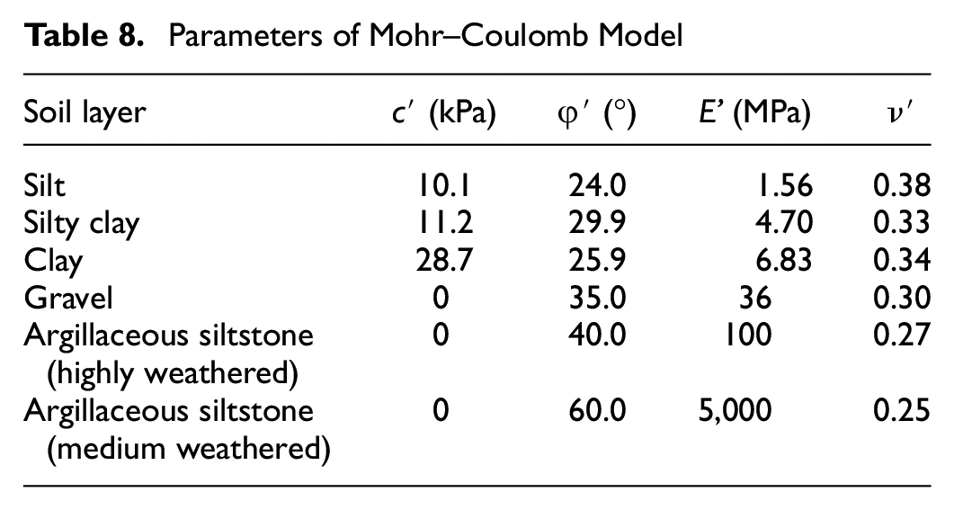
In the numerical model, the silt, silty clay, and clay adopted M-C model and the HSS model for deformation analysis. The result is compared with the monitoring data to evaluate its performance. The parameters of the M-C model for each soil layer are shown in Table 8, and other parameters such as underground diaphragm walls, reinforced concrete supports, and engineering piles are obtained from the code for the design of concrete structures (GB50010-2010) and shown in Table 9.

Table 8.

Parameters of Mohr–Coulomb Model

Soil layer	c′ (kPa)	φ′ (°)	E' (MPa)	ν′
Silt	10.1	24.0	1.56	0.38
Silty clay	11.2	29.9	4.70	0.33
Clay	28.7	25.9	6.83	0.34
Gravel	0	35.0	36	0.30
Argillaceous siltstone(highly weathered)	0	40.0	100	0.27
Argillaceous siltstone (medium weathered)	0	60.0	5,000	0.25

Table 9.

Other Material Parameters

Category	Unit weight (kN·m⁻³)	Elasticity modulus (GPa)	Poisson’s ratio
Underground diaphragm wall	25	31.5	0.15
Enclosing purlin and reinforced concrete support	25	30	0.20
Engineering piles	25	30	0.20

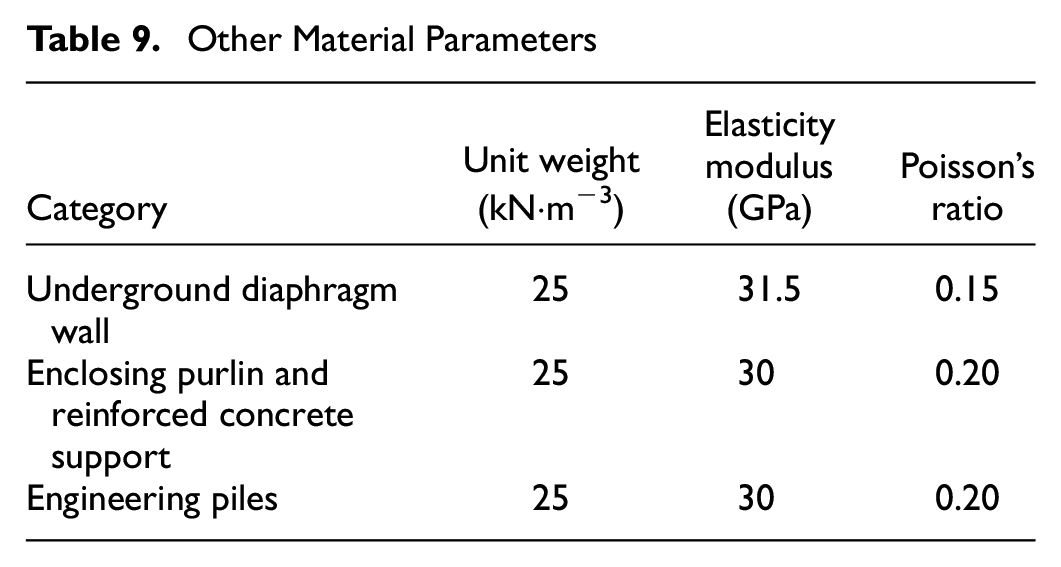
Figure 9 presents a comparison between the numerical analysis results and the monitoring data for the lateral displacement of the underground diaphragm wall at monitoring points LCX1 and LCX12. The monitoring points LCX1 and LCX12, located at the center of the short and long sides of the foundation pit (i.e., one side of the north pit), respectively, are considered representative locations. Figure 9 depicts several typical working conditions. Specifically, completion of the third floor excavation, indicates that all soft soil layers in the foundation pit are excavated. The completion of the fifth floor excavation indicates the excavation of the southern foundation pit to the end. The completion of the eighth floor excavation indicates the excavation of the northern foundation pit to the end. The numerical analysis results obtained using the M-C model exhibit significant deviations from the measured deformation. In contrast, the deformation prediction based on the HSS model is considerably more accurate than that of the M-C model. Furthermore, the numerical analysis results obtained using in situ G^ref₀ exhibit a higher level of accuracy in predicting deformation, particularly in the soft soil layers before the completion of the third floor excavation, as compared with the results obtained using indoor G^ref₀.

Figure 9.

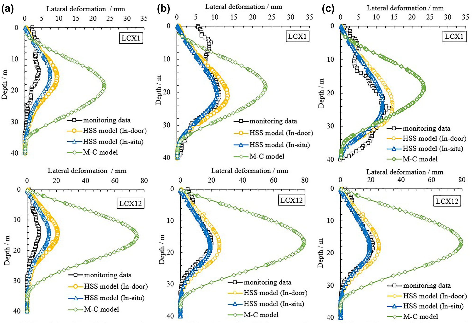
Comparative analysis of lateral deformation of diaphragm wall: (a) completion of the third floor excavation; (b) completion of the fifth floor excavation; and (c) completion of the eighth floor excavation.

A detailed analysis of Figure 9 shows that the lateral deformation of the underground diaphragm wall increases with increasing excavation depth when the relatively weak soil layer is excavated (before the completion of the fifth floor excavation). The depth of maximum deformation also increases with excavation depth, and the maximum lateral deformation of the underground diaphragm wall typically occurs near the current excavation surface. However, during excavation of the gravel and argillaceous siltstone layers, the lateral deformation of the underground diaphragm wall remains relatively stable or slightly increases with increasing excavation depth. The depth at which the maximum deformation occurs does not significantly deepen further. The HSS model accurately reflects this deformation trend, which is consistent with the measured data. In contrast, the M-C model fails to capture this phenomenon.

Before the completion of the excavation for the third layer, the lateral displacement of the diaphragm wall, as determined through numerical analysis employing the HSS model, exceeded the measured displacement. Notably, the lateral displacement simulated using the in situ parameter G^ref₀ was smaller than that derived from the simulation using the indoor test parameter G^ref₀. Although this simulation was closer to the measured value, it still exhibited a magnitude greater than the measured displacement. This may be because the upper layer is dominated by soft soil, which is easily disturbed during sampling and testing, resulting in the physical and mechanical parameters obtained from the indoor test (when simulated with the in situ parameter G^ref₀, the other parameters are still the indoor test parameters) being smaller than those in the in situ state, and thus the lateral displacements obtained from the numerical simulation are larger.

Conclusion

This study presents the HSS model parameters of the main soil layers involved in a significant engineering project in the western region of Hangzhou. The numerical results obtained from the HSS model are compared with both monitoring data and numerical analysis results obtained using the M-C model. Numerical results of indoor G^ref₀ and in situ G^ref₀ are compared and analyzed while keeping the other parameters of the HSS model unchanged. The main conclusions are as follow:

(1) The experimental values of the HSS model parameters for the primary soil layers in the western region of Hangzhou are within the statistical range of previous literature results. However, some of the values are close to the statistical limits and slightly different from the mean. This observation suggests that there are regional variations in the properties of the soil layers.

(2) The accuracy of numerical analysis using the HSS model in predicting the deformation of the foundation pit enclosure structure is significantly higher than that of M-C model, and the prediction results are closer to the measured data.

(3) Numerical results using in situ G^ref₀ are closer to actual measurements than indoor G^ref₀, resulting in a higher deformation prediction accuracy. Consequently, it is recommended that the method of in situ testing be prioritized to obtain relevant HSS model parameters.

(4) Numerical analysis using the HSS model effectively captures the lateral deformation behavior of the underground diaphragm wall with excavation depth. The analysis results are consistent with the measured values, whereas the M-C model cannot reflect these relevant laws.

Footnotes

Author Contributions

The authors confirm contribution to the paper as follows: study conception and design: Minmin Luo; data collection: Minmin Luo, Jiasheng Huang, Yun Chen; analysis and interpretation of results: Yun Chen, Jiasheng Huang; draft manuscript preparation: Yun Chen, Danyi Shen. All authors reviewed the results and approved the final version of the manuscript.

Declaration of Conflicting Interests

The author(s) declared no potential conflicts of interest with respect to the research, authorship, and/or publication of this article.

Funding

The author(s) disclosed receipt of the following financial support for the research, authorship, and/or publication of this article: This work is financially supported by the Construction of scientific research project in Zhejiang Province (2023K089, 2023K195).

ORCID iDs

Jiasheng Huang

Panpan Shen Habib

References

Chu

Y.-s.

Liang

F.-y.

Y.-d.

Numerical Analysis of Deformation of Deep Excavation Adjacent to Metro Considering Small-Strain Stiffness of Soil. Chinese Journal of Rock Mechanics and Engineering, Vol. 29, Supplement 1, 2010, pp. 3184–3192.

Kung

G. T.-c.

Jheng

U.-z.

Evaluation of Analyzing Excavation-Induced Wall Deflection and Ground Movement Using Hardening Soil Models. Chinese Journal of Geotechnical Engineering, Vol. 32, Supplement 2, 2010, pp. 175–178.

Shao

Jiang

Chen

J.-y.

S.-k.

J.-x.

Wei

C.-h.

Deformation of Deep Foundation Pits Due to Excavation and Dewatering Based on HSS Model and Modified Cam-Clay Model. Journal of Hydraulic Engineering, Vol. 46, Supplement 1, 2015, pp. 231–235.

Khorasani

Soleimani-Javid

Arshid

Lampani

Civalek

Ö.

Thermo-Elastic Buckling of Honeycomb Micro Plates Integrated with FG-GNPs Reinforced Epoxy Skins with Stretching Effect. Composite Structures, Vol. 258, 2021, p. 113430.

Ikbarieh

Izadifar

M. A.

Abu-Farsakh

M. Y.

Voyiadjis

G. Z.

A Parametric Study of Embankment Supported by Geosynthetic Reinforced Load Transfer Platform and Timber Piles Tip on Sand. Transportation Geotechnics, Vol. 38, 2023, p.100901.

Wang

W.-d.

Wang

H.-r.

Z.-h.

Experimental Study of Parameters of Hardening Soil Model for Numerical Analysis of Excavations of Foundation Pits. Chinese Journal of Rock and Soil Mechanics, Vol. 33, No. 8, 2012, pp. 2283–2290.

Liang

F.-y.

Jia

Y.-j.

Ding

Y.-j.

Huang

M.-s.

Experimental Study on Parameters of HSS Model for Soft Soils in Shanghai. Chinese Journal of Geotechnical Engineering, Vol. 36, No. 2, 2017, pp. 269–278.

Zong

L.-d.

Z.-h.

Weng

Q.-p.

Wang

W.-d.

, Application of Small Strain Constitutive Model in the Analysis of an Ultra Large and Deep Excavation. Chinese Journal of Underground Space and Engineering, Vol. 15, Supplement 1, 2019, pp. 231–242.

Khasib

I. A.

Nik Daud

N. N.

Izadifar

M. A.

Consolidation Behaviour of Palm-Oil-Fuel-Ash-Based Geopolymer Treated Soil. Geotechnical Research, Vol. 10, No. 3, 2023, pp. 138–152.

10.

Izadifar

M. A.

Luo

Abu-Farsakh

M. Y.

Chen

Performance Evaluation of Design Methods for Geosynthetic-Reinforced Pile-Supported Embankments. Transportation Research Record: Journal of the Transportation Research Board, 2023. 2677: 458–475.

11.

Benz

Small Strain Stiffness of Soils and Its Numerical Consequences. University of Stuttgart, 2006.

12.

Luo

M. M.

Chen

Zhou

Research Status and Prospect of Parameter Selection for the HS-Small Model. Industrial Construction, Vol. 51, No. 4, 2021, pp. 172–180.

13.

Bolton

M. D.

The Strength and Dilatancy of Sands. Géotechnique, Vol. 36, No. 1, 1986, pp. 65–78.

14.

Brinkgreve

R. B. J.

Broere

Plaxis Material Models Manual. Delft University of Technology Press, 2006.

15.

Gao

D.-Z.

Wei

D.-D.

Z.-X.

Geotechnical Properties of Shanghai Soils and Engineering Applications. Marine Geotechnology and NearShore/Offshore Structures, Vol. 923, 1986, pp. 161–177.

16.

Janbu

Soil Compressibility as Determined by Cedometer and Triaxial Tests. Proc., 3rd European Conference on Soil Mechanics and Foundation Engineering, Wiesbaden, Vol. 1, 1963, pp. 19–25.

17.

Z.-h.

Wang

J.-h.

Wang

W.-d.

Analysis of a Complicated Deep Excavations Supported by Substructures. Chinese Jourmal of Geotechnical Engineering, Vol. 28, Supplement 1, 2006, pp. 1355–1359.

18.

D.-l.

Chen

Dai

Wang

Z.-y.

Liang

Numerical Study of Dig Sequence Effects During Large-Scale Excavation. Applied Sciences, Vol. 13, 2023, p. 11342.