Comparison of Pavement Roughness Indicators from Traditional Inertial Profilers and Emerging Connected Vehicle Sensors

Abstract

This study is an evaluation of the consistency and potential of crowdsourced connected vehicle (CV) data as an alternative to traditional inertial profiler (IP) measurements for road roughness evaluation. IP data were collected from three roadway corridors, SH 21, SH 6, and FM 2818, in Bryan, Texas, which comprised a variety of pavement types and functional classifications. Lane-specific international roughness index (IRI) values were recorded using a calibrated inertial profiler and analyzed at every 10 ft. These were compared with direction level ride values collected at an average spacing of 82 ft from a third-party CV data provider. A general agreement was found between IP and CV data on asphalt and concrete surfaces, but there were substantial differences between seal coat sections, where CV ride values overestimated roughness by 80–100 in./mi. A grouping analysis was conducted to compare segments categorized by roughness level from both datasets. The results showed a moderate match in identifying the roughest segments by the CV system, compared with those identified by IP. This match rate varied by profile and improved with broader grouping sizes. Results show that CV data might have greater sensitivity to vehicle behavior (for example, braking at intersections), while IP-based systems are calibrated to record actual road roughness. This could be one of the reasons for the moderate mismatch in identifying rougher segments using the two methods. Despite these limitations, the CV system’s high frequency of measurements, especially on highways, demonstrates its potential for cost-effective, network-level pavement monitoring.

Keywords

roadway infrastructure connected vehicle data inertial profilers road performance measures roughness

Introduction

Road condition monitoring is essential to estimate maintenance needs and ensure an acceptable level of service. There have been various measures to monitor road condition, but the commonly used metric is the international roughness index (IRI). The IRI is used to quantify road roughness and is a critical input in road asset management. Many of the state roadway agencies measure IRI once a year, owing to time and effort constraints ( 1 ). As some roads degrade faster than others, the lack of timely data can delay maintenance interventions. However, annual IRI data collected using inertial profilers (IPs) may fail to capture rapid deterioration, such as pothole formation, or sudden changes in road condition resulting from traffic diversions and recent maintenance treatments. To overcome this problem, various practitioners are interested in harnessing the power of original equipment manufacturer (OEM) sensor data from connected vehicles (CVs). CV data are produced from operating vehicles within the fleet and thereby reduce the burden for data collection. These platforms collect data more frequently and on a larger scale, allowing for timely and cost-effective monitoring ( 2 ).

This paper presents an examination of the evaluation of IRI data produced by a third-party vendor that collects crowdsourced CV data to generate ride condition metrics. It explores, in detail, how ride quality and IRI measurements obtained through different methods (i.e., using CVs and calibrated inertial profilers) relate to each other. The analysis also identifies areas of divergence to trace the origins of discrepancies back to the methods employed. Additionally, the paper discusses whether the crowdsourced approach could potentially replace traditional IRI measurements in the long term and serve as a more affordable method for continuous roadway condition monitoring.

Objective

This study includes an analysis, comparing IRI values obtained from a calibrated inertial profiler with pavement roughness data produced from OEM connected vehicles sensors.

The analysis is designed to address the following key objectives.

Evaluate the consistency between CV-derived roughness values and lane-specific IRI measurements collected by an inertial profiler.

Assess the accuracy of CV sensors in capturing localized pavement roughness, focusing on their ability to identify very rough and very smooth segments.

Explore the potential advantages of CV roughness data, including broader spatial coverage, higher frequency of updates for network-level pavement condition monitoring.

Through this comparative analysis, the aim is to determine the reliability of CV sensors as a supplementary or alternative technology to conventional IRI data collection methods in pavement condition assessment.

Literature Review

Transportation agencies spend trillions of dollars maintaining road infrastructure based on a worst-first approach. But studies show that an alternative preserve-first approach will maintain assets and reduce preservation costs by three times, thus saving hundreds of billions of dollars ( 3 ). However, a preserve-first approach requires more frequent monitoring to forecast optimum maintenance triggers. Traditionally, roads are monitored using profilometers, which detect road profiles along pavements ( 4 ). But these profilers could be costlier relative to the budget allotted by the roadway agencies. Therefore, these systems are often used as a component of complex roadway systems, such as freeways and highways, generally where speeds are higher than 50–60 mph.

There have been various studies to research alternative ways to monitor roads, such as using image processing, unmanned aerial vehicles (UAVs), lidar (light detection and ranging technology), and inertial sensors. Much research has been done on analyzing roadway images using machine learning (ML) techniques, such as computer vision. Several authors have used ML models or fine-tuned image-based models for roadway anomaly detection. Arya et al. ( 5 ) used roadway imagery data from four countries—USA, Japan, India, and the Czech Republic—and prepared a large-scale annotated database comprising more than 25 000 images. Bashar and Torres-Machi ( 6 ) used deep learning models on publicly available satellite imagery to estimate pavement roughness. Abohamer et al. ( 7 ) used a convolution neural network (CNN) to classify rough pavement sections and estimate pavement roughness using surface images. To capture comprehensive pavement profiles, Gao et al. ( 8 ) used lidar to acquire three-dimensional point cloud data to evaluate the longitudinal and lateral variation in pavement roughness. In addition, there have been some affordable solutions for data collection, which utilize low-cost sensors, such as accelerometers and gyroscope sensors. Mirtabar et al. ( 9 ) developed a cost-effective sensing unit suitable for crowdsourcing, processing vertical acceleration data into pavement profiles to calculate the IRI. These calculated values were validated against ground truth measurements collected by a high-accuracy laser road surface profiler (RSP) on identical routes. The study established the system’s accuracy through a linear regression analysis between the two datasets, achieving a coefficient of determination of 0.82.

Connected vehicle data approaches have gained momentum, owing to their scalability. With advancement in sensing technologies, vehicles in general use are becoming increasingly better at data collection. This leads to crowdsourcing such vibration data; this is extensive and inexpensive and has high sampling frequency, making it suitable for large-scale pavement roughness evaluation. But not much information is available on the vehicles, because privacy laws make it difficult to standardize the process of data collection. Liu et al. ( 10 ) developed a semisupervised learning model to deal with incomplete data and multivehicle fusion. To isolate road roughness from mechanical issues, Liu et al. mathematically modeled engine vibrations as harmonic processes and incorporated them in the model’s intercept, distinguishing them from the random signal of pavement roughness. Additionally, a self-training model was designed to estimate IRIs iteratively across the network, while quantifying the coupled effect of sampling rate and vehicle quantity on the model’s overall accuracy ( 10 ). This is a significant challenge to researchers and practitioners as vehicle dynamics can influence roughness reporting. If the original manufacturers of CV ride data do not account for vehicle-induced vibration, this would be an inherent limitation of the dataset.

Some studies have explored connected vehicle data and address changes in roadway data. Mathew et al. ( 11 ) developed spatial and temporal variations out of 3 billion connected vehicle records in Indiana. The data, which spanned 30 months, revealed changes in roadway conditions on miles of interstate roads. Mahlberg et al. ( 12 ) studied over 70 mi of Interstate-65 in Indiana using both inertial profiler and connected vehicle production data. They established a linear relationship between both data sources with a correlation factor, R², of 0.79, suggesting that connected vehicle data can be used as a viable tool. Various studies have been conducted to examine alternatives to traditional IRI data collection and monitoring; among these, connected vehicle data look a promising alternative. But very few studies have compared them with the traditional IRI methodology using IP data and investigated how the CV data could complement or become a replacement. This study will be an exploration of how road profiles collected from these two data sources vary over different roadway types and are able to indicate bad profile sections.

Data Collection

Ground truth data were collected using a calibrated inertial profiler to ensure accuracy and consistency in pavement condition measurements. The data collection was conducted across three distinct roadway corridors located in the Bryan–College Station region in Texas: state highway (SH) 21, SH 6, and farm-to-market road (FM) 2818. These routes were purposefully selected to represent a diverse range of roadway classifications, including controlled-access highways, general highways, and arterial roadways.

SH 21 is classified as an arterial roadway and spans approximately 3.3 mi. It features a combination of divided and undivided segments, offering a varied cross-sectional profile typical of urban arterials. The profile has a mix of concrete and asphalt pavement surfaces measuring 1.5 mi and 1.8 mi, respectively. SH 6, by contrast, is a fully access-controlled highway corridor extending for approximately 11.5 mi with complete asphalt layered pavement. It represents a high-capacity roadway designed for uninterrupted traffic flow. FM 2818 serves as a 4.7-mi-long highway corridor and, similar to SH 21, contains both divided and undivided segments, making it a representative sample of the suburban highway type. This profile again had a mix of concrete and asphalt sections, measuring 0.7 mi and 4 mi, respectively, and also included a concrete bridge deck.

IRI measurements were collected on both the innermost and outermost lanes in each travel direction across all three roadway corridors. This detailed lane-specific methodology resulted in the development of 12 distinct IRI profiles, accounting for the two lanes in each direction along each route. By capturing data at this granular level, the analysis can better reflect lane-level variability in pavement roughness.

In contrast, the CV data provider generated IRI-equivalent profiles (called ‘rides’ and measured in inches per mile) for each direction of travel only, without differentiating between individual lanes. As a result, the CV dataset comprised six ride profiles, corresponding to the two directions across the three roadway segments. Therefore, there is a data collection difference: the IP IRI data were lane-specific and the CV ride data were direction-specific.

The IRI profile data collected using the inertial profiler provided measurements at a high resolution, with IRI values recorded every 1 in. and aggregated every 10 ft along the roadway. In comparison, the ride data collected from the connected vehicles system were reported at a coarser resolution, with ride values generated at an average spacing of 82 ft. To allow for a direct comparison between the two datasets, the high-resolution IRI data from the profiler were reprocessed to produce values at the same 82-ft intervals as the CV ride data. This step ensured that both datasets represented the same segment locations along the roadway.

As shown in Figure 1, the CV ride segments were aligned with the corresponding IP IRI segments for comparison. For each segment, the midpoint was used to represent the average condition of that segment. These midpoints were then matched across the two datasets using a distance-based approach. Specifically, the midpoint of each IRI segment was connected to the nearest CV ride segment, as long as it fell within a distance equal to the length of the segment. This method helped ensure that only closely located segments were compared, improving the accuracy of the analysis.

Figure 1.

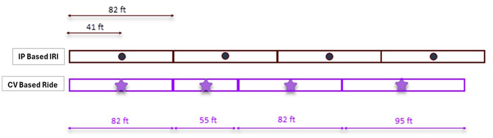
Alignment of inertial profile (IP) international roughness index (IRI) segments and connected vehicle (CV) ride segments for comparison.

By standardizing segment lengths and aligning midpoints, a consistent framework was established for comparing the road roughness results from both measurement methods.

A small number of IP IRI segments could not be joined to corresponding CV ride segments. This was primarily because of differences in segment lengths and slight misalignments of the start and end points of the profiles. Since the IP IRI and CV ride data were collected independently, their total profile lengths did not always align perfectly, leading to some mismatch at the start and end limits of the routes. Additionally, the overall lengths of the IRI and ride profiles varied slightly across the corridors. These discrepancies resulted in unmatched segments, particularly near the ends of the roadway sections, where one dataset might extend farther than the other. As a result, those unmatched segments were excluded from the comparison analysis to maintain consistency and accuracy in the evaluation. Table 1 presents the number of CV ride segments joined to IP IRI segments. Close to 98% of the CV ride segments were spatially aligned with the IP IRI segments.

Table 1.

No. of CV Ride Segments Joined to IP IRI Segments

Profile description	No. of IRI segments	No. of CV ride segments joined to IP IRI segments	CV ride segments correctly mapped to IP IRI segments, %
FM2818 northbound inner lane	304	299	98
FM2818 southbound outer lane	305	296	97
SH21 eastbound outer lane	214	206	96
SH21 westbound inner lane	215	209	97
SH6 northbound inner lane	739	728	99
SH6 southbound outer lane	740	732	99
Total number of segments	2517	2470	98

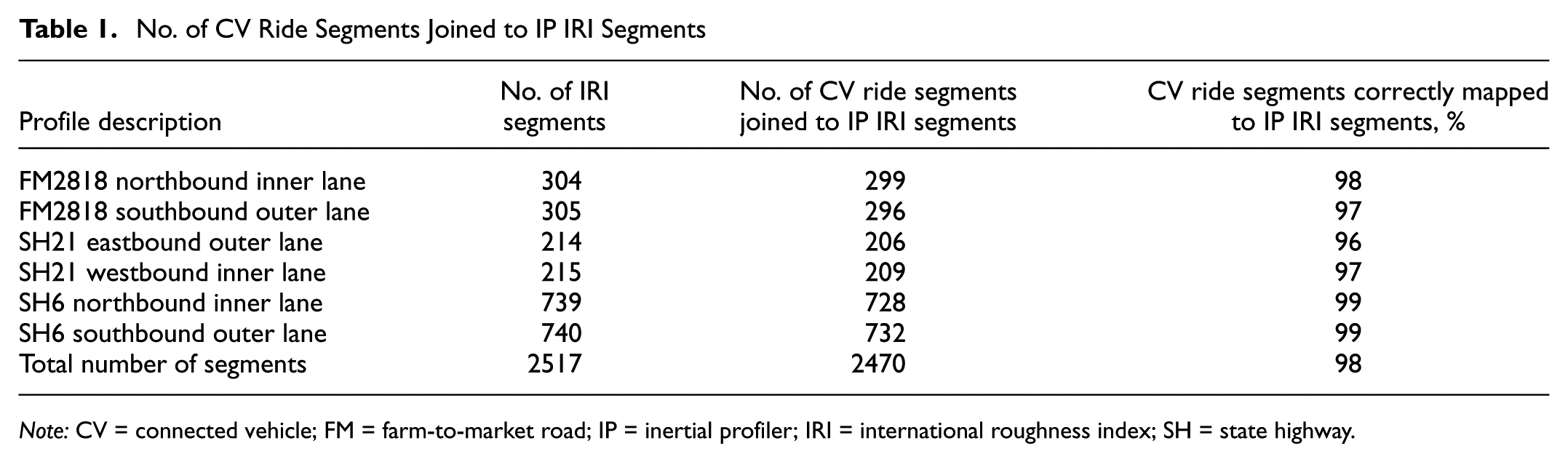
Note: CV = connected vehicle; FM = farm-to-market road; IP = inertial profiler; IRI = international roughness index; SH = state highway.

Number of Observations from CV Crowdsourced Platform

The CV system generates daily roughness profiles by collecting data from a fleet of connected vehicles equipped with onboard sensors. These vehicles travel across the road network as part of their regular operations. The raw data from these trips include measurements related to vehicle motion and road surface interaction. Before any analysis is performed, these data are processed through a standardized filtering system. This filtering process is designed to ensure that only reliable and consistent data are used in generating roughness estimates. Once filtered, the data are aggregated on a weekly basis. To account for daily variations in traffic patterns, vehicle types, and environmental conditions, the data provider aggregates the raw inputs into a weekly average. This preprocessed metric, referred to by the vendor as a ‘long-term roughness’ estimate, is designed to smooth out short-term fluctuations and yield a more consistent measure of pavement condition over time. Furthermore, the provider’s proprietary filtering process inherently applies a speed threshold to ensure accuracy. Consequently, data collected at very low speeds, typically below 15 mph, were excluded from the delivered dataset.

Additionally, the number of usable observations varies from segment to segment, depending on traffic volumes, vehicle routes, and data coverage. However, the CV system used in this study does not report the exact number of observations associated with each individual segment. Instead, average observation counts are used to provide a general sense of data availability. For example, in the case of SH 21 (Figure 2), the long-term roughness estimate is based on an average of 157 weekly observations per segment. This means that data were collected consistently across several years, giving approximately three years of observation data in total.

Figure 2.

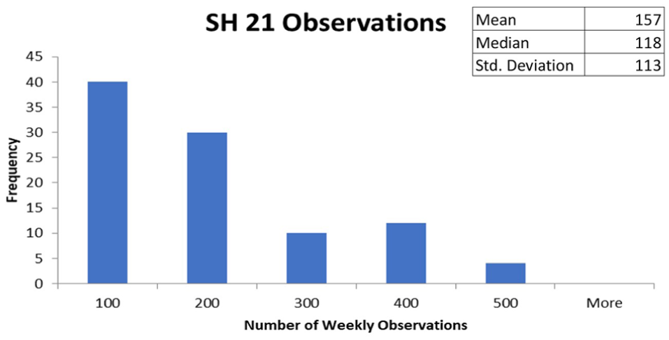
Frequency of weekly observations of state highway (SH) 21 segments.

As shown in Figure 3, the number of weekly observations used to calculate pavement roughness was higher for FM 2818, compared with SH 21. On average, each segment along FM 2818 received approximately 350 weekly observations, more than twice the number recorded for SH 21. This higher volume of data contributes to greater statistical confidence in the roughness estimates for FM 2818 and suggests a higher flow of connected vehicles along that corridor.

Figure 3.

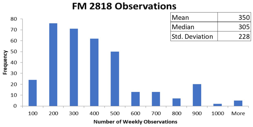
Frequency of weekly observations of farm-to-market road (FM) 2818 segments.

As shown in Figure 4, SH 6 had the highest number of weekly observations of the three roadways studied. SH 6 is an access-controlled highway and carries more daily traffic than FM 2818 and SH 21. Because of this higher traffic volume, more connected vehicle data were collected on this route. On average, each segment of SH 6 received about 1632 weekly observations. This large amount of data was used to calculate the long-term roughness. The high number of observations helps improve the accuracy and reliability of the roughness results for SH 6. It also makes SH 6 the best-covered roadway in this analysis.

Figure 4.

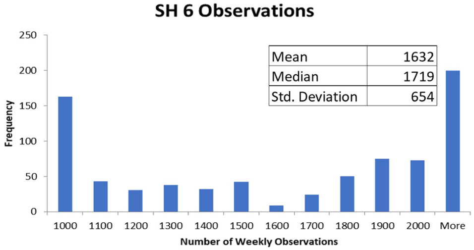
Frequency of weekly observations of state highway (SH) 6 segments.

Highway-type roads generally had higher weekly observations for CV measurements compared with arterial roads, such as SH 21, owing to higher annual average daily traffic (AADT) and greater penetration of connected vehicles in the fleet. Little information on how many total observations per segment was collected or filtered for the aggregated weekly observation, owing to the proprietary system of the CV data provider.

Analysis

To ensure consistency in the comparative analysis, both IRI and ride profiles were trimmed and spatially aligned to match at their respective start and end points. This preprocessing step was essential to eliminate discrepancies caused by differences in total profile lengths or recording boundaries.

The CV ride profiles were then compared against the IP IRI lane-specific profiles, which included data from both the inner and outer lanes. In addition to analyzing each lane individually, an average IRI profile was generated by averaging the inner and outer lane measurements. This averaged profile was also compared with the directional ride values reported by the connected vehicles data provider.

The analysis was aimed to determine which IRI profile most closely aligns with the CV ride data by evaluating the CV roughness data against several representations of IP IRI measurements of inner lane, outer lane, and averaged lane roughness. This comparison provides insight into the representativeness of the connected vehicle directional roughness data and their potential to approximate lane-specific IP IRI data.

Road Condition Classification

For the Moving Ahead for Progress in the 21st Century Act (MAP-21), the Federal Highway Administration classifies pavement conditions based on IRI in three categories ( 13 ):

good: IRI less than 95 in./mi

fair: IRI between 95 and 170 in./mi

poor: IRI greater than 170 in./mi.

While this classification scheme is useful for national-level reporting and performance monitoring, it was determined to be too coarse for the specific analytical needs of this study. The broad thresholds did not adequately capture the variation in pavement performance observed across the study corridors, particularly when assessing lane-level and segment-specific roughness. To address this limitation, the original categories were refined into a four-tiered system. By introducing the ‘very good’ (<60 in./mi) category, we were able to conduct a more granular sensitivity analysis to see if the CV sensors could distinguish between ‘smooth’ and ‘very smooth’ pavements. We do not suggest replacing MAP-21, for official compliance. This reclassification allows for a granular assessment of pavement conditions and supports more precise comparisons between measurement methodologies:

very good: IRI less than 60 in./mi

good: IRI between 60 and 95 in./mi

fair: IRI between 95 and 170 in./mi

poor: IRI exceeds 170 in./mi.

Using the revised classification system, all segments from the collected profiles were categorized according to their corresponding IRI values. A total of six profiles were analyzed, comprising 2470 individual segments (Table 2). Among these, 949 segments were classified as being in very good condition, 948 segments in good condition, 466 segments in fair condition, and 107 segments in poor condition. Notably, SH 21 contained the highest number of segments classified as poor, indicating a greater degree of surface deterioration along this route. In contrast, SH 6 and FM 2818, both highway-type corridors, had very few segments rated as poor, suggesting generally better pavement performance. Given the relatively higher concentration of poor-condition segments in the SH 21 profile, this roadway was selected for further detailed analysis. Focusing on SH 21 enables a more targeted evaluation of roughness detection accuracy under more challenging surface conditions, where the variability in IRI values is more pronounced.

Table 2.

Number of Segments in Each IRI Classification of All Six Profiles

Profiles	Very good	Good	Fair	Poor	Total segments
FM2818 northbound	69	151	71	8	299
FM2818 southbound	68	162	59	7	296
SH21 eastbound	11	31	109	55	206
SH21 westbound	27	66	92	24	209
SH6 northbound	422	250	48	8	728
SH6 southbound	352	288	87	5	732
Total segments	949	948	466	107	2470

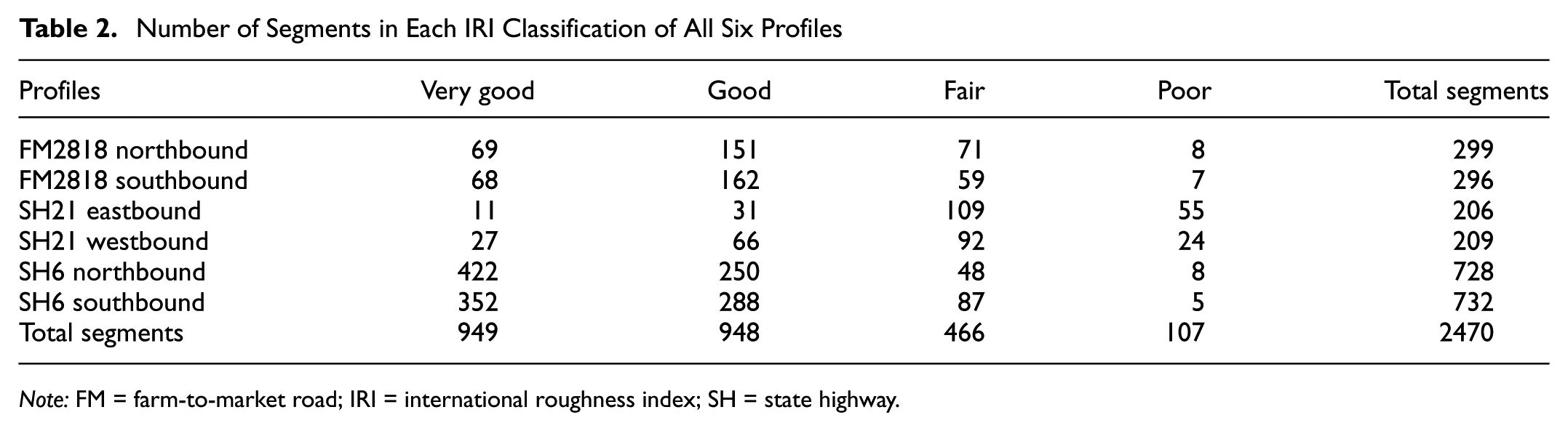
Note: FM = farm-to-market road; IRI = international roughness index; SH = state highway.

Outer Lane Profiles

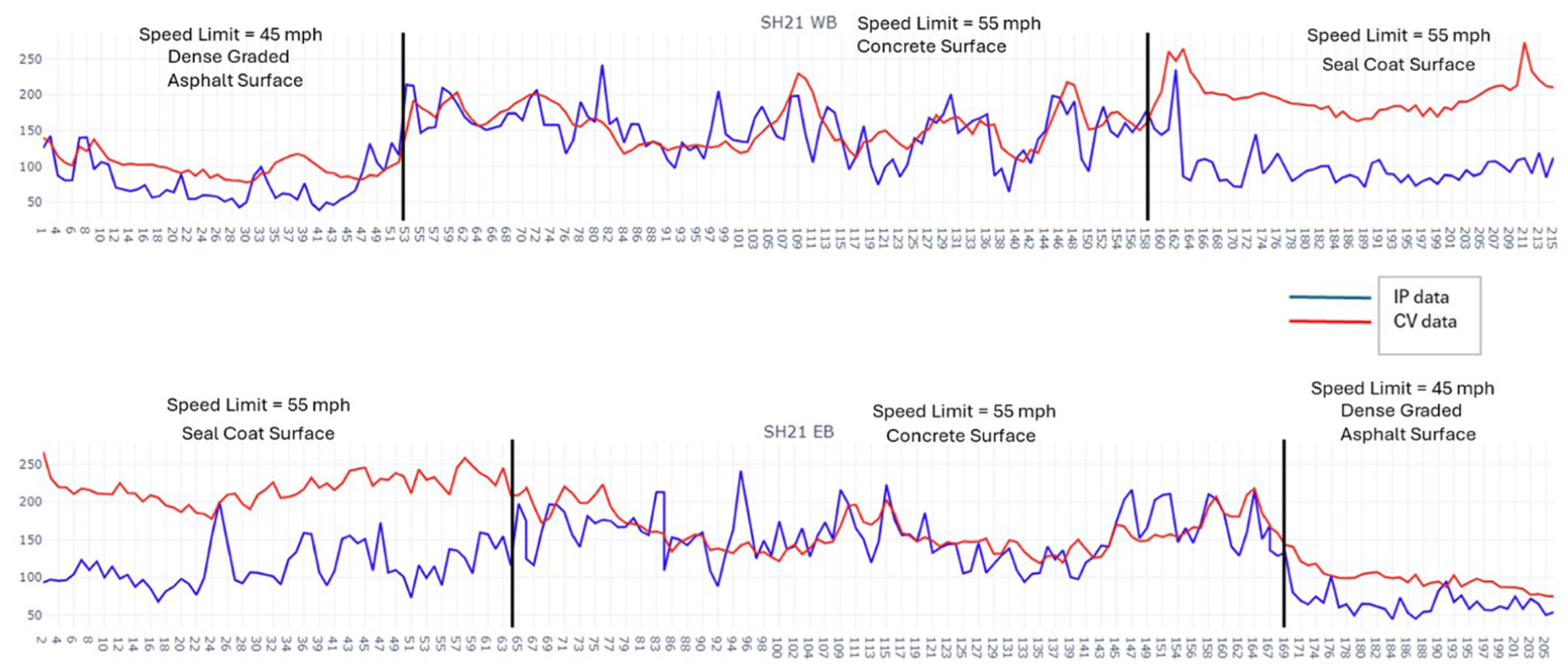
In this section, the IP IRI data from the outer lanes of SH 21 were compared with the corresponding CV ride values, with the analysis conducted separately for westbound and eastbound directions (Figure 5). The alignment focused specifically on outer lane profiles for each direction. In the westbound outer lane, the data indicated the presence of two distinct speed limit zones and three different pavement surface types. A similar observation was made in the eastbound direction, where two speed limits and three surface types were also identified.

Figure 5.

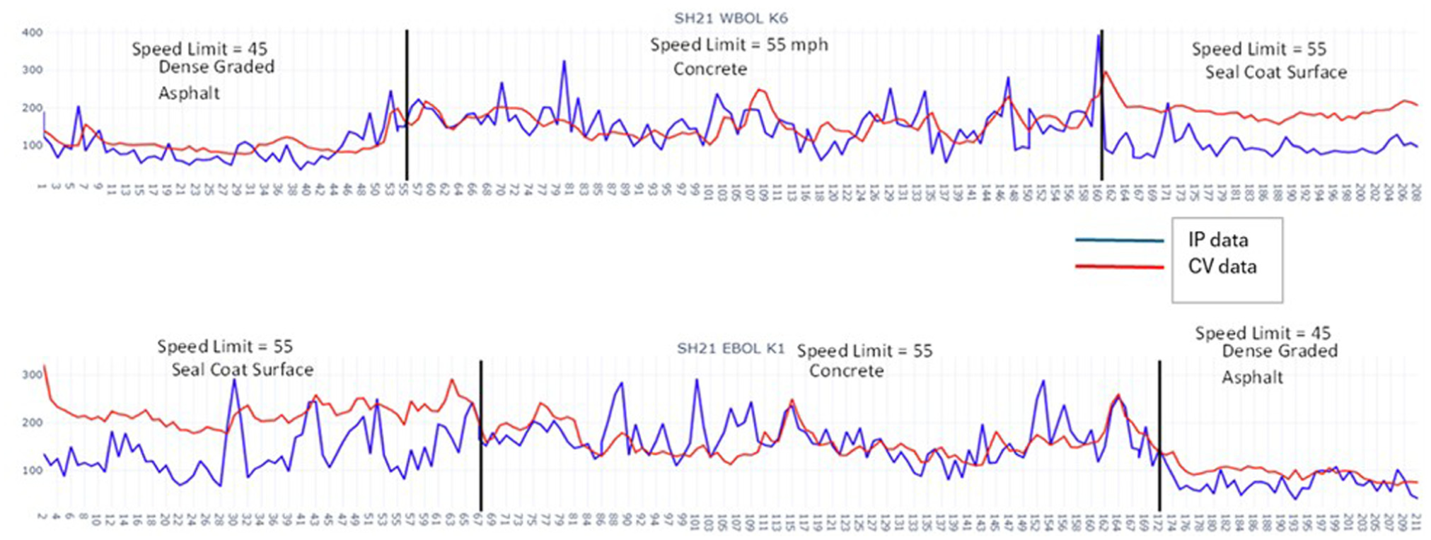
Connected vehicle (CV) and inertial profiler (IP) profiles of state highway (SH) 21, westbound and eastbound outer lane.

When comparing the IP IRI profiles with the CV ride values, the results showed general agreement across asphalt and concrete pavement sections. However, significant discrepancies were observed in areas where seal coat surfaces were applied. In these sections, the CV rides indicated roughness levels approximately 80–100 in./mi higher than those reported by the inertial profiler. This difference highlights a potential limitation in the calibrated profiler’s sensitivity to certain surface textures, particularly those associated with chip seals.

Another notable observation was that both profiles exhibited a sharp increase in roughness at the transition points between different surface materials. These transitions were marked by distinct vertical lines on the profile plots. This finding is consistent with observations made by Pike and Wilson ( 14 ), who studied the effect of audible lane departure warning treatments on seal-coated pavements. Their research demonstrated that vehicles traveling over chip seals at higher speeds experienced increased levels of noise and vibration. Pike and Wilson concluded that chip seals inherently generate more ambient noise than other surface types and more aggressive treatments may be required to mitigate these effects. The divergence between IP IRI and CV ride measurements in seal coat sections may be attributed to the different nature of data capture. While the calibrated inertial profiler is designed to filter out vehicle-induced vibrations and noise, CV captures raw sensor inputs that may better reflect the subjective experience of ride quality from a user’s perspective. As such, the CV data may offer valuable insights into how drivers perceive roughness, especially in sections where surface texture plays a dominant role in ride discomfort.

Inner Lanes

This section is focused on the analysis of the inner lanes and evaluates how CV-derived roughness values compare against the IP-derived IRI data for these lanes. Visually, the IP IRI values for the inner lanes appear consistently lower than those recorded for the outer lanes (Figure 6). This observation aligns with typical pavement performance patterns, as inner lanes are generally subjected to lower traffic volumes and less frequent heavy vehicle loading, resulting in smoother surface conditions.

Figure 6.

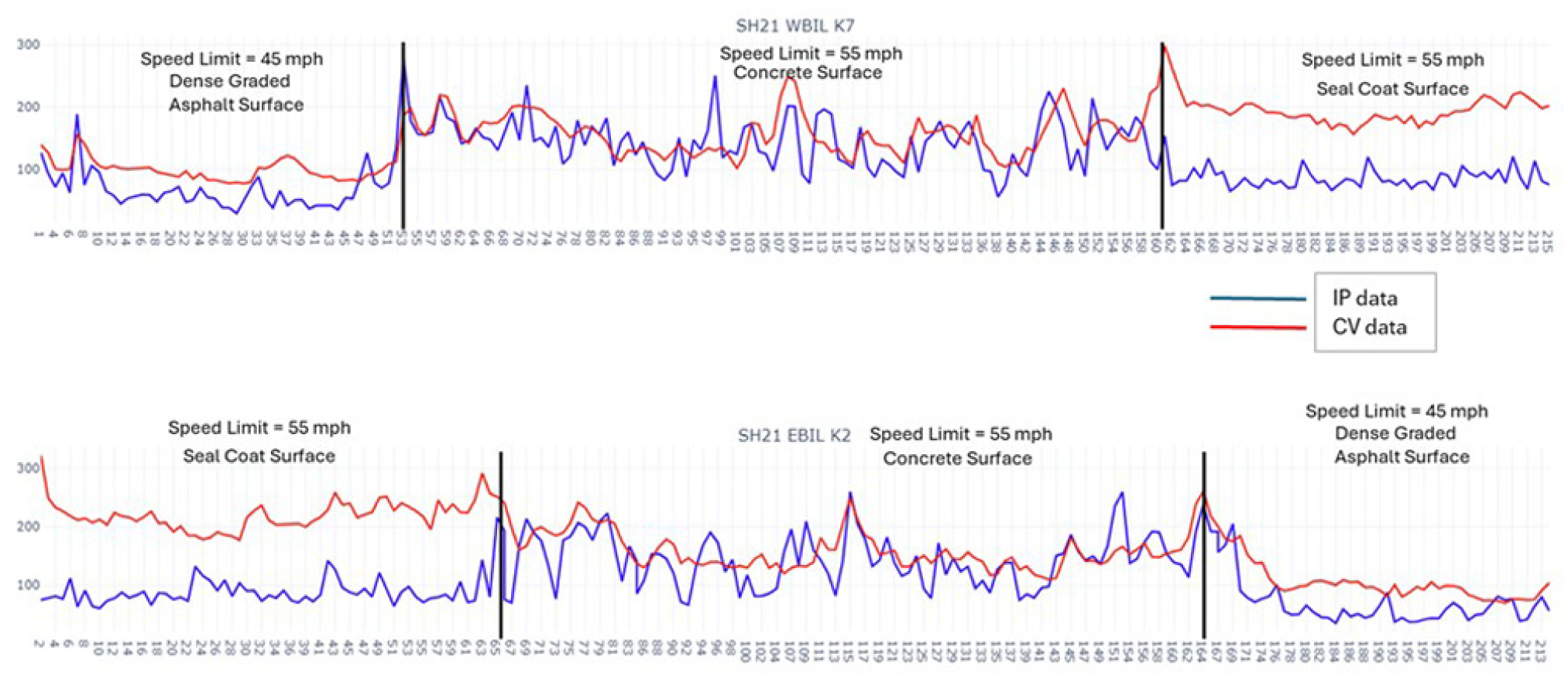
Connected vehicle (CV) ride and inertial profiler (IP) profiles of state highway (SH) 21, westbound and eastbound inner lane.

When comparing the CV ride profiles with IP IRI inner lane data, a noteworthy observation emerges. The CV ride profile appears to follow the IP IRI peaks more closely on concrete surface sections, capturing many of the same localized variations in the ride values. This level of agreement was not as evident in comparison with outer lane profiles, where discrepancies, particularly over seal coat sections, were more pronounced. Since passenger cars are driven more frequently in inner lanes, the CV system probably captures more data for these lanes than for outer lanes. However, we could not correlate observation counts with accuracy because the CV data were limited to directional attributes and did not include lane-specific positioning.

Averaged Profile of Both Inner and Outer Lanes

To address the spatial resolution discrepancy between the lane-specific IP data and the directional CV data, an averaged IP profile was computed by calculating the simple average of the inner and outer lane IRI values for each segment. We assumed that this profile (Figure 7) could provide a closer equivalent to the directional nature of the CV dataset, but no distinguishable similarity was observed with this comparison.

Figure 7.

Connected vehicle (CV) ride, and averaged inner and outer lane inertial profiler (IP) international roughness index profiles of state highway (SH) 21, westbound and eastbound.

Ranking Worst Segments

The goal of this part of the analysis was to check whether both IRI and CV ride profiles identified the same road segments as the worst for roughness. To do this, all segments were ranked based on their IP IRI and CV ride values. A higher IRI means more roughness, so the segment with the highest IRI was given Rank 1, marking it as the worst segment in that profile.

This ranking process was followed separately for each dataset. Segments were first sorted from highest to lowest IRI values and then given a rank. The same process was repeated using the CV ride values. Since some profiles had more than 700 segments and others had fewer than 200, it was very unlikely that the exact same segment would be ranked the worst in both datasets.

Instead of comparing the exact rank of each segment, segments were grouped into categories based on how high they ranked. For example, segments in the top 5%, 10%, or 25% roughness values were grouped together. These groups were then compared across the IP IRI and CV ride data to see if the same segments consistently appeared among the roughest parts of the roadway. This approach gave a more realistic way to check if both methods were in agreement on the worst segments (i.e., highest roughness within the corridor).

Grouping Analysis

As shown in Table 3, all segments were divided into five groups of 500 segments each to compare roughness rankings between IP IRI and CV ride datasets. These groups were created based on decreasing roughness levels, with Group 1 (G1) representing the segments with the highest IRI and ride values (i.e., the roughest surfaces) and Group 5 (G5) representing those with the lowest roughness values (i.e., the smoothest surfaces).

Table 3.

Grouping Analysis of All Segments

		CV-based ride data					No. of segments
Group description		G1: very high IRI, %	G2: high IRI, %	G3: medium IRI, %	G4: low IRI, %	G5: very low IRI, %	No. of segments
IP-based IRI data
	G1: very high IRI	41	34	17	6	2	500
	G2: high IRI	29	25	26	10	10	500
	G3: medium IRI	20	21	24	20	15	500
	G4: low IRI	8	15	19	33	25	500
	G5: very low IRI	3	6	13	34	44	470

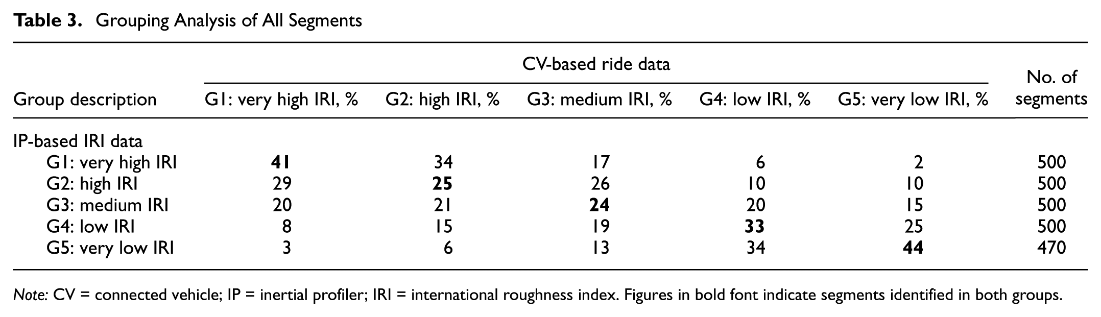
Note: CV = connected vehicle; IP = inertial profiler; IRI = international roughness index. Figures in bold font indicate segments identified in both groups.

The comparison was focused on how many of the 500 roughest segments identified by the CV (G1) were also present in the IP IRI Group G1. The results showed that only 41% of the segments identified by the CV as being in G1 matched with the IP IRI G1 segments. These percentages have been typeset in bold font (located diagonally) in Table 3 to emphasize the level of agreement between the two datasets. The remaining CV-identified G1 segments were distributed across the other IRI groups: 34% were found in G2, 17% in G3, 6% in G4, and the remaining 2% in G5.

While the 41% match in G1 indicates moderate agreement, the analysis does not account for how close the mismatched segments were to the group boundary. For example, some segments identified by CV-based ride data in G2 might have narrowly missed being included in IP-based IRI data G1. This raises an important question: Are these mismatches caused by slight differences in ranking thresholds, or do they represent significant disagreement between the two data sources? A deeper analysis of segment proximity to group boundaries (Figure 8) was conducted to understand the nature of these partial mismatches more accurately.

Figure 8.

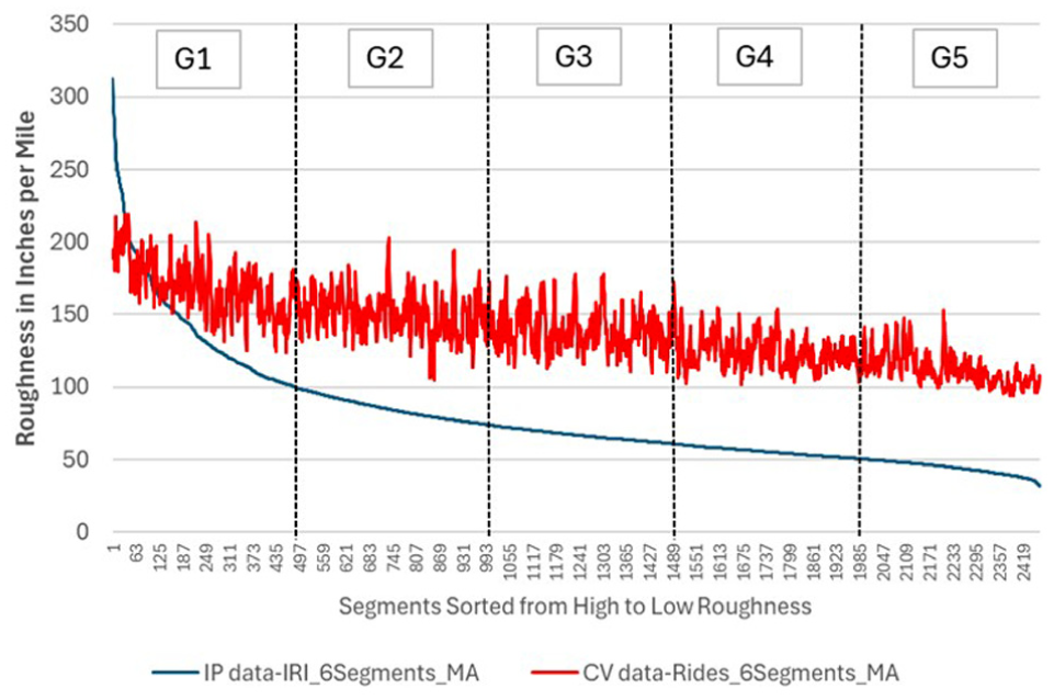
Segments sorted in decreasing order of inertial profiler (IP)-based international roughness index (IRI) and connected vehicle (CV)-based ride.

To explore this further, Figure 8 presents the segment profiles for both IP-based IRI and CV-based ride, with segments sorted in descending order of roughness. Both are moving average (MA) trends that show how each method measures roughness, from the roughest segments to the smoothest segments. A six-segment moving average was calculated to smoothen out the roughness to 0.1-mi intervals. The IP-based IRI trendline exhibits a sharp initial decline, indicating that only a small number of segments exhibit extremely high roughness, followed by a rapid transition to more moderate roughness values. In contrast, the CV-based ride trendline shows a more gradual decline, with a majority of segments in moderate roughness. Group G1 comprised all the poor-rated segments and the majority of fair-rated segments. This visual distinction suggests that while the IP-based IRI identifies a smaller subset of segments as being in critical condition, the CV-based ride distributes roughness more broadly across a larger number of segments. The IP-based method was better at identifying the worst segments of the bad segments than was the CV-based method.

Of all three roads, SH 21 contained the highest number of poor-condition segments (see Table 2); therefore, it was selected for detailed analysis. Figure 9 illustrates the 20 worst-ranked segments based on roughness, as identified independently based on IP-based IRI and CV-based ride. Segments highlighted in red represent those identified based on IRI, while segments in blue represent those identified based on CV ride. The segment colors overlap where both sources identify the same segment among their respective top 20, indicating agreement between the two data sources.

Figure 9.

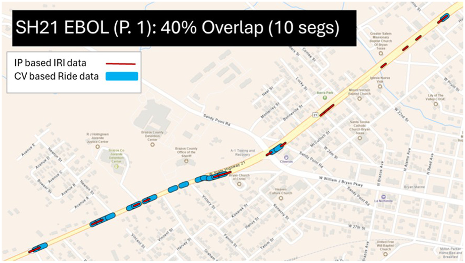
State highway (SH) 21 eastbound outer lane profile.

Figure 9 shows that while there is some overlap, several red and blue segments do not coincide, suggesting differences in how the two systems detect and rank roughness. Specifically, for the SH 21 eastbound outer lane profile, only 40% of the worst 25 segments identified by the CV system match those identified by the IRI system.

An additional observation is that several of the segments marked as very rough by the CV-based ride tend to appear at roadway turns or near signalized intersections. These areas might be typically associated with vehicle deceleration, where drivers apply braking force. Such maneuvers might influence the vehicle’s acceleration profile, which is a key input in the CV system’s estimation of ride quality. As a result, the braking-induced vibrations might have been captured by vehicle acceleration sensors and interpreted as increased roughness. This could explain why the CV system identifies certain segments as rough that are not similarly ranked by the calibrated inertial profiler, which is designed to filter out transient vehicle dynamics unrelated to pavement conditions.

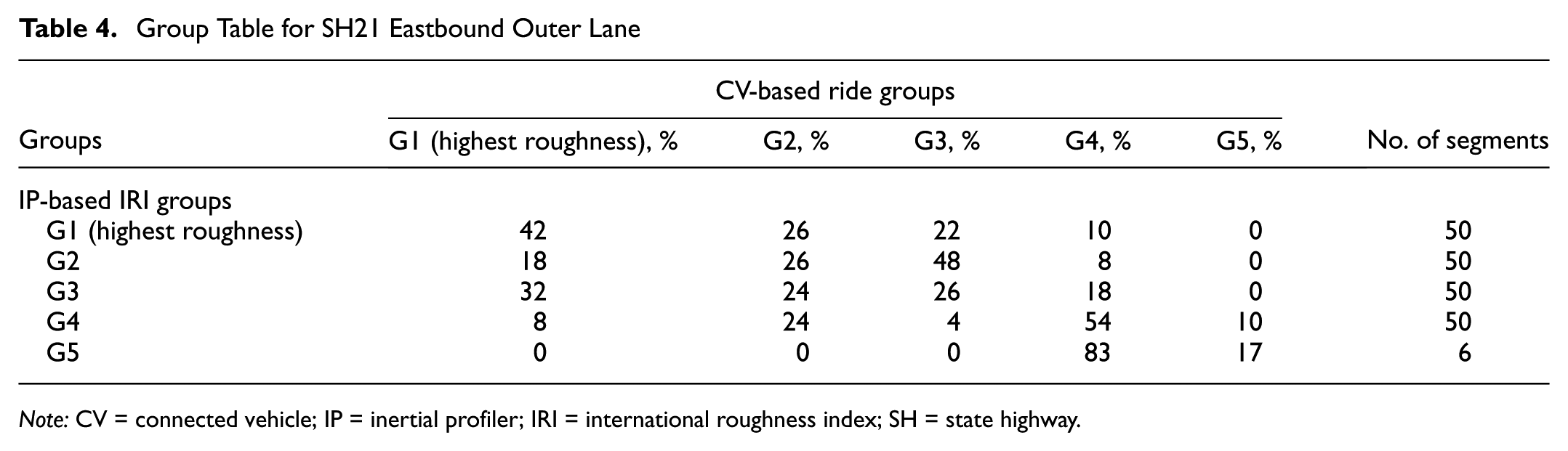
The grouping analysis was repeated for a single profile, SH 21 eastbound outer lane, using smaller group sizes to allow a closer comparison (Table 4). Segments were ranked by roughness, and the top 200 segments were divided into four groups of 50 segments each. The top 50 segments identified by the IRI system were called Group 1 (G1). These were compared with CV system’s rankings. Out of the top 50 roughest segments, measured by IP-based IRI, 42% were also ranked in the top 50 roughest segments, measured by CV-based ride. Another 26% were found in the CV’s Group 2 (ranks 51–100), 22% in Group 3 (ranks 101–150), and 10% in Group 4 (ranks 151–200).

Table 4.

Group Table for SH21 Eastbound Outer Lane

Groups	CV-based ride groups					No. of segments
Groups	G1 (highest roughness), %	G2, %	G3, %	G4, %	G5, %	No. of segments
IP-based IRI groups
G1 (highest roughness)	42	26	22	10	0	50
G2	18	26	48	8	0	50
G3	32	24	26	18	0	50
G4	8	24	4	54	10	50
G5	0	0	0	83	17	6

Note: CV = connected vehicle; IP = inertial profiler; IRI = international roughness index; SH = state highway.

This result shows a similar pattern to the earlier analysis: some segments are matched closely, but others are spread across nearby rank groups. This may result from differences in how each method measures or interprets roughness at the segment level.

As discussed earlier, grouping analysis was performed using segments from all profiles combined and from individual profiles. In each case, different group sizes were tested, depending on the total number of segments available. As seen in Figure 8, the CV system was able to identify rough segments across the dataset but did not consistently pinpoint the very worst segments, compared with IP-based IRI data.

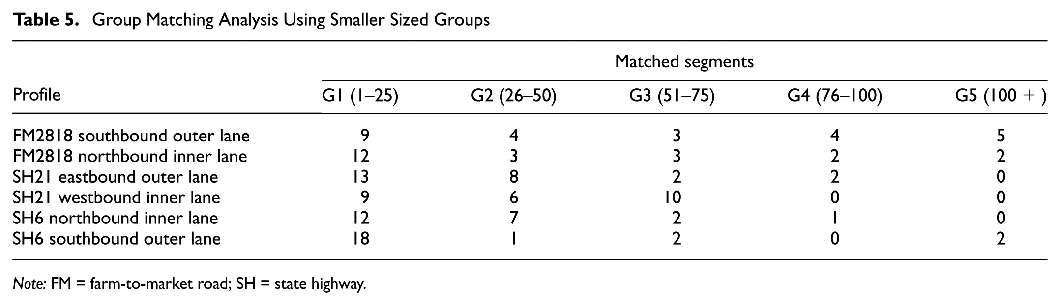
To investigate this further, a smaller group size was tested to see if the CV system could match the IP-based IRI worst 25 segments more closely. Table 5 shows the results of this analysis. Of the top 25 worst segments (Group 1), concerning IRI, 18 segments were also found in the CV’s top 25 on SH 6. This was the highest level of agreement observed across all profiles. This high match rate can be attributed to the roadway classification as a fully access-controlled highway, designed for uninterrupted traffic flow. Unlike the arterial routes, this corridor minimizes vehicle maneuvers, such as braking and turning, which were previously identified as primary sources of noise in the CV roughness estimates. Additionally, SH 6 is probably driven by the substantial volume of crowdsourced data on this corridor, which averaged 1632 weekly observations per segment (Figure 4), compared with significantly lower counts on other routes. This high frequency of observations might smooth out transient errors, resulting in greater statistical confidence and a better match in groups G1 and G2.

Table 5.

Group Matching Analysis Using Smaller Sized Groups

Profile	Matched segments
Profile	G1 (1–25)	G2 (26–50)	G3 (51–75)	G4 (76–100)	G5 (100+)
FM2818 southbound outer lane	9	4	3	4	5
FM2818 northbound inner lane	12	3	3	2	2
SH21 eastbound outer lane	13	8	2	2	0
SH21 westbound inner lane	9	6	10	0	0
SH6 northbound inner lane	12	7	2	1	0
SH6 southbound outer lane	18	1	2	0	2

Note: FM = farm-to-market road; SH = state highway.

In comparison, the other profiles showed 13 or fewer matches within their top 25 segments, meaning that, in most cases, fewer than 50% of IRI’s worst segments were identified by the CV system. Although crowdsourced ride data from CV can identify general areas of poor pavement, the results do not fully align with calibrated IRI measurements when pinpointing the absolute worst segments. Therefore, while CV systems are useful for broader network-level assessments, they might be less precise for detecting the most critical roughness zones at the segment level.

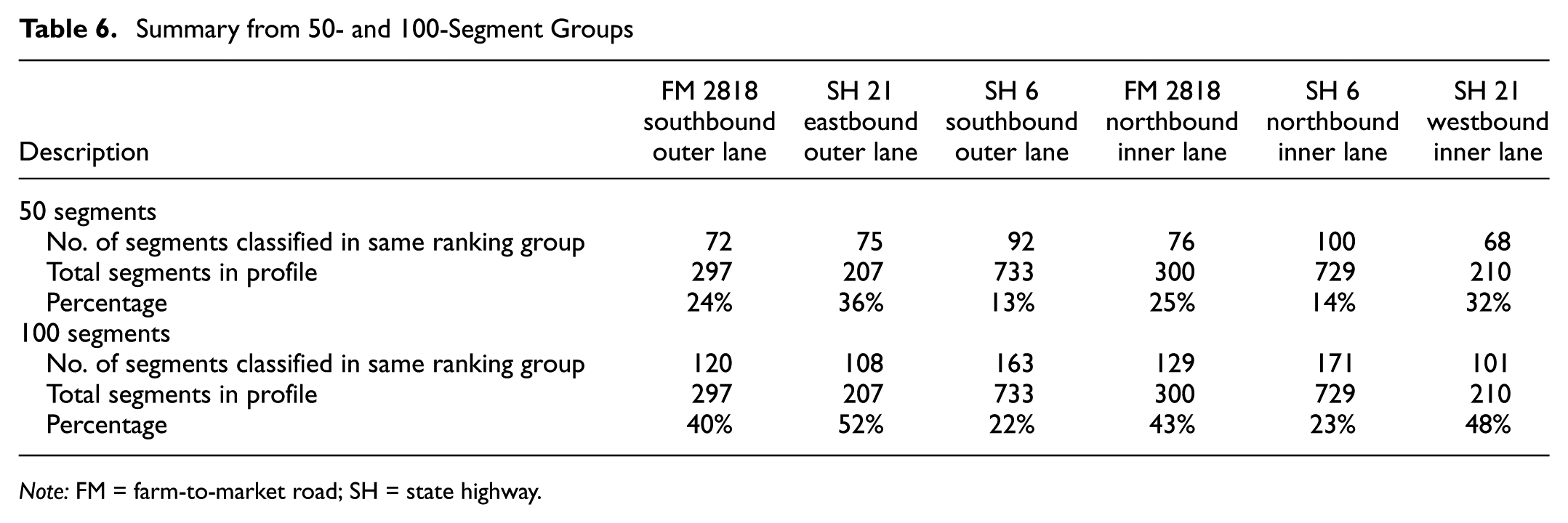
This analysis was also repeated using larger group sizes, specifically groups of 50 and 100 segments, to see whether the CV system could capture more of the same rough segments identified based on IRI when broader groupings were used. The goal was to test if increasing the group size would improve the agreement between the two datasets. Table 6 summarizes the number of segments that were classified in the same ranking group, or roughness level, by both measurement systems. The results are consistent with earlier observations. For the SH 21 eastbound profile, 36% of the segments were classified in the same group when using 50-segment groupings. When the group size was increased to 100 segments, the match rate increased to 52%.

Table 6.

Summary from 50- and 100-Segment Groups

Description	FM 2818 southbound outer lane	SH 21 eastbound outer lane	SH 6 southbound outer lane	FM 2818 northbound inner lane	SH 6 northbound inner lane	SH 21 westbound inner lane
50 segments
No. of segments classified in same ranking group	72	75	92	76	100	68
Total segments in profile	297	207	733	300	729	210
Percentage	24%	36%	13%	25%	14%	32%
100 segments
No. of segments classified in same ranking group	120	108	163	129	171	101
Total segments in profile	297	207	733	300	729	210
Percentage	40%	52%	22%	43%	23%	48%

Note: FM = farm-to-market road; SH = state highway.

While this increase was expected, as larger groups allow for more overlap, the improvement was modest. In all other profiles, the percentage of matched segments remained below 50%, even with the larger group size. This indicates that although the CV system can generally identify rough sections of the roadway, it does not fully align with the IRI profiler data in classifying segments at finer resolution, even when broader groupings are applied.

Conclusion

This study showed that roughness values crowdsourced from CVs do not fully match IRI values measured using a certified inertial profiler. The CV system was able to show general pavement roughness trends, but it did not always agree with IP-based IRI when identifying the roughest road segments. This difference probably arises because of how the two systems measure and process data.

The CV system was effective at separating smooth roads from rough ones. However, it had difficulties identifying the difference between roads that were poor and those that were very poor, concerning roughness. The match between CV-based ride and IP-based IRI results also depended on the type of road surface. On asphalt and concrete surfaces, the results were closer, but on chip seal or seal coat surfaces, there were bigger differences. Chip seals create more vibration, which the CV sensors detect and can possibly consider as incorrect roughness. The profiler is designed to ignore these effects. This means that CV systems might reflect what a driver feels more than the actual roughness of the road.

The study addresses the fundamental difference in spatial resolution, where traditional IP measurements are lane-specific (inner versus outer) while CV data were aggregated at a directional level. To evaluate the accuracy of this directional proxy, the analysis compared CV ride values against three distinct IP baselines: the inner lane, the outer lane, and an averaged profile of both lanes. The study identified that directional CV data aligned more closely with inner lane profiles rather than those of the outer lanes. This trend could arise because of the general trend that passenger vehicles favor inner lanes over outer lanes. However, the lack of lane-specific positioning in the CV data prevented a formal verification of this correlation.

Vehicle speed also affected the CV system’s results. To ensure data consistency, the provider’s proprietary filtering system inherently excluded data collected below 15 mph. While this removes some noise from braking and turning, the threshold is lower than traditional inertial profiling standards. As a result, the CV system often showed high roughness near intersections or turns. These values might reflect vehicle behavior, not the pavement condition, which led to disagreement with IP-based IRI data in those areas.

One of the biggest advantages of CV systems is the high frequency of data collection. It uses connected vehicles to gather daily roughness readings. These are filtered and averaged weekly to show pavement trends. This is much more frequent than traditional IRI surveys, which usually occur once a year. For example, on SH 6, each segment had about 1600 weekly CV observations.

On SH 21 eastbound outer lane, only 42% of the roughest 50 segments identified based on IRI were also identified by the CV system. In smaller groups, such as the top 25, the match rate dropped even more. Larger group sizes, such as the top 100, improved the match slightly. This shows that the CV system is more effective in identifying overall trends in pavement roughness than in finding the roughest parts of the road.

Recommendations and Future Work

Based on the results of this study, crowdsourced CV data demonstrate significant potential as a supplementary tool for network-level ride quality assessments. Although the current system cannot yet replace certified inertial profiler measurements for exact reporting, it offers a scalable and cost-effective alternative for local agencies constrained by budget. These agencies can explore implementing a continuous network screening approach to effectively distinguish between smooth and rough pavements. This allows for a hybrid monitoring strategy where low-cost CV data scans the entire network to identify trends, enabling agencies to prioritize visual inspections and deploy expensive certified equipment only to specific locations that require detailed engineering analysis.

Future work should be planned to further explore the unique capabilities of CV systems to function as an early warning mechanism. Unlike annual inspections, weekly updates from CV data can capture rapid road deterioration caused by weather or traffic events long before scheduled maintenance. Additionally, the potential of CV data to capture the user experience needs to be investigated further, as the system detects vibrations from rough textures or braking that traditional equipment is designed to ignore. To fully realize this potential, future research must address implementation hurdles to facilitate the use of CV ride data within transportation agencies. This includes exploring data procurement methods, defining cost structures, and establishing robust data governance and quality control frameworks to ensure reliability. Technical refinements are also needed to improve the spatial resolution of CV data from directional aggregates to lane-specific metrics to better align with maintenance planning.

Footnotes

Acknowledgements

The authors gratefully acknowledge the collaborative and financial support of the Strategic Initiatives and Innovation Division of the Texas Department of Transportation. In particular, Benjamin McCulloch has been highly supportive of this research and evaluation effort.

Authors’ Note

The authors utilized Google Gemini 3 Pro exclusively for grammatical refinement and stylistic editing within the literature review section. This tool was not used for literature search, content generation, data collection, or data analysis. In accordance with TRB and COPE guidelines, the authors have verified the accuracy, validity, and appropriateness of the edited text and assume full responsibility for the content of the manuscript.

Author Contributions

The authors confirm contribution to the paper as follows: study conception and design: Vivek Kumar Gupta, Charles Gurganus, Shawn Turner; data collection: Charles Gurganus; analysis and interpretation of results: Vivek Kumar Gupta, Joel Ben Thomas, Charles Gurganus, Michael Martin, Shawn Turner, Nasir Gharaibeh; draft manuscript preparation: Vivek Kumar Gupta, Charles Gurganus, Nasir Gharaibeh. All authors reviewed the results and approved the final version of the manuscript.

Declaration of Conflicting Interests

The authors declared no potential conflicts of interest with respect to the research, authorship, and/or publication of this article.

Funding

The authors disclosed receipt of the following financial support for the research, authorship, and/or publication of this article: financial support by the Strategic Initiatives and Innovation Division of the Texas Department of Transportation.

ORCID iDs

Vivek Kumar Gupta

Joel Ben Thomas

Charles Gurganus

Michael Martin

Shawn Turner

Nasir Gharaibeh

References

Aleadelat

Ksaibati

Estimation of Pavement Serviceability Index Through Android-Based Smartphone Application for Local Roads. Transportation Research Record, 2017, 2639: 129–135. https://doi.org/10.3141/2639-16

Bridgelall

A Connected Vehicle Approach for Pavement Roughness Evaluation. Journal of Infrastructure Systems, Vol. 20, No. 1, 2014, p. 04013001.

Ram

P. V.

Zimmerma

K. A.

Borthakur

A. J.

Mugabe

K. B.

Raghunathan

Demonstrating the Application of Life Cycle Planning (LCP) on a Pavement Network: Results from the Arizona DOT Pavement Pilot Project. Report No. FHWA-HIF-21-044, Federal Highway Administration, 2021. www.fhwa.dot.gov/asset/pubs/hif21044.pdf

Loprencipe

de Almeida Filho

F. G. V.

de Oliveira

R. H.

Bruno

Validation of a Low-Cost Pavement Monitoring Inertial-Based System for Urban Road Networks. Sensors, Vol. 21, No. 9, 2021, p. 3127. https://doi.org/10.3390/s21093127

Arya

Maeda

Ghosh

S. K.

Toshniwal

Mraz

Kashiyama

Sekimoto

Deep Learning-Based Road Damage Detection and Classification for Multiple Countries. Automation in Construction, Vol. 132, 2021, p. 103935. https://doi.org/10.1016/j.autcon.2021.103935.

Bashar

M. Z.

Torres-Machi

Deep Learning for Estimating Pavement Roughness Using Synthetic Aperture Radar Data. Automation in Construction, Vol. 142, 2022, p. 104504. https://doi.org/10.1016/j.autcon.2022.104504.

Abohamer

Elseifi

Dhakal

Zhang

Fillastre

C. N.

Development of a Deep Convolutional Neural Network for the Prediction of Pavement Roughness from 3D Images. Journal of Transportation Engineering, Part B: Pavements, Vol. 147, No. 4, 2021, p. 04021048. https://doi.org/10.1061/JPEODX.0000310.

Gao

Fan

Wei

Liu

Differences Evaluation of Pavement Roughness Distribution Based on Light Detection and Ranging Data. Applied Sciences, Vol. 13, No. 14, 2023, p. 8080. https://doi.org/10.3390/app13148080.

Mirtabar

Golroo

Mahmoudzadeh

Barazandeh

Development of a Crowdsourcing-Based System for Computing the International Roughness Index. International Journal of Pavement Engineering, Vol. 23, No. 2, 2022, pp. 489–498. https://doi.org/10.1080/10298436.2020.1755434.

10.

Liu

Large-Scale Pavement Roughness Measurements with Vehicle Crowdsourced Data Using Semi-Supervised Learning. Transportation Research Part C: Emerging Technologies, 2021, 125: 103048. https://doi.org/10.1016/j.trc.2021.103048.

11.

Mathew

J. K.

Desai

Sakhare

R. S.

Hunter

Bullock

D. M.

Spatiotemporal Analysis of Pavement Roughness Using Connected Vehicle Data for Asset Management. Journal of Transportation Technologies, Vol. 15, No. 1, 2024, pp. 1–16. https://doi.org/10.4236/jtts.2025.151001.

12.

Mahlberg

J. A.

Zachrisson

Leslie

D. K.

Bullock

D. M.

Pavement Quality Evaluation Using Connected Vehicle Data. Sensors (Basel, Switzerland), Vol. 22, No. 23, 2022, p. 9109. https://doi.org/10.3390/s22239109.

13.

Simpson

A. L.

Rada

G. R.

Visintine

Groeger

Guerre

Improving FHWA’s Ability to Assess Highway Infrastructure Health: Development of Next Generation Pavement Performance Measures. Report No. FHWA-HIF-13-042. U.S. Department of Transportation Federal Highway Administration Office of Asset Management, Washington, D.C., 2013.

14.

Pike

A. M.

Wilson

B. T.

Evaluation of Audible Lane Departure Warning Treatments on Seal Coats. Transportation Research Record, 2019, 2673: 826–839. https://doi.org/10.1177/0361198119850458.