Mandatory Construction Temperature as a Specification for Integral Abutment Bridges

Abstract

Integral abutment bridges (IABs) experience significant cyclic thermal movements induced by fluctuating temperatures. The pattern and maximum value of these movements depend on bridge properties, specific locality of bridge, and the initial temperature when the bridge starts behaving integrally, called the installation temperature or construction temperature (CT). Current practices mostly focus on design temperatures and lack standardized requirements for initial CT. Potential discrepancies may arise because specifications for design temperatures have a tacit assumption that CT is grossly near the middle of the extreme bridge temperatures. However, actual CT can significantly deviate from this tacit assumption during the construction phase because it is mostly not mandated. Consequently, bridge movements may become significantly asymmetrical and unwanted. This study addresses this gap by proposing a practical and easily applicable methodology for setting and mandating CT as a specification to be jointly implemented during in both design and construction of IABs. The output of the proposed method is a tight range for CT, applicable to most days without significant adverse effects in construction scheduling. Attaching the CT as a criterion into design protocols may result in enhanced predictions of thermal displacements and internal forces within IABs. Ultimately, theoretical assumptions can be connected to their practical implementation. As a result, valuable insights and actionable recommendations may be achieved to enhance the reliability, longevity, and efficiency of IABs through overall performance improvements. The methodology presented can also be used for other structures where thermal displacements are of concern.

Keywords

integral abutment bridges initial construction temperature thermal loadings

Introduction

Abutments and superstructures of integral abutment bridges (IABs) act as a single structural unit because expansion joints or sliding bearings are eliminated. A change in temperature causes a bridge superstructure to expand or contract, resulting in thermal-induced movement. This movement applies lateral loading and unloading forces to the bridge substructure comprising abutment, pile, and backfill. Cyclic thermal movements also cause changes in earth pressures behind abutments, which may vary from minimum active to maximum passive, depending on the abutment displacement pattern. Thus, cyclic thermal displacements have significant effects on the performance of IABs, as shown in previous experiments by Kim and Laman, and Peric et al., numerical studies by Kim and Laman, and reported damage of in in-service bridges during field observations by Murphy and Yarnold, and Lee et al. ( 1 – 5 ). Therefore, it is evident that the magnitude of thermal displacement controls the extent of thermal performance of IABs. Understanding the significance of initial construction temperature (CT) in IABs is pivotal, as it directly influences the magnitude of thermal displacements, which, in turn, determines thermal loads.

As known well by bridge engineers, the magnitude of thermal displacement is influenced by the coefficient of thermal expansion, length of bridge superstructure, and temperature fluctuations realized. The fluctuations in temperature are primarily governed by the initial CT for the specific location where bridge is erected. This initial CT governs temperature fluctuations of an IAB, and, therefore, its movement pattern. However, current practices do not strictly mandate a value or a range for initial CT, and a tacit assumption for CT is common. In the U.S., AASHTO advises a temperature range to define the change in temperature for determining thermal displacement, regardless of the actual value of CT ( 6 ). In Canada, when specific site data is unavailable, an effective CT of 15°C (60°F) is assumed for both steel and concrete bridges by the Canadian Standards Association (CSA) ( 7 ). According to the Eurocode enacted by the European Committee for Standardization (Comité Européen de Normalisation [CEN]), CT is defined as the initial temperature of the bridge ( 8 ). In cases where the initial temperature is unpredictable, the average temperature during construction period is considered instead. The initial temperature value may be specified for an individual project or in standard codes and specifications. In the absence of available information, the initial temperature may be assumed to be 10°C. When uncertainty exists about the bridge’s sensitivity to initial temperature, it is advisable to consider both a lower and upper limit for expected initial temperature.

Design specifications in the U.S., Canada, and Europe generally lack specific lower or upper bounds for mandating the CT of bridges. This causes discrepancies, as specified design temperatures may deviate from the tacit assumption made for CT because CT can be any value during the course of the construction phase if it is not restricted. As the actual CT deviates from the design assumption, bridge movements may become significantly asymmetrical and unwanted during either one of the expansion or contraction cycles. As a result, assumptions made for CT during the design state and the actual CT experienced during the construction in field may mismatch. The main goal of the thermal design task should be to obtain bridge movements which are as symmetrical as possible during the seasonal cycles, which cannot be achieved without incorporating the actual CT.

The literature validating bridge design specifications for temperature ranges is limited. In one study, field testing was undertaken on two bridges in Iowa, aiming to monitor air and bridge temperatures along with other parameters ( 9 ). The findings revealed that the temperature range specified by AASHTO Standard Specifications 1983 ( 10 ), was notably smaller than the measured temperature ranges for both bridges ( 10 ). The researchers also reported displacement measurements of the Maple River Bridge as 22.5 mm (0.9 in.) expansion versus 40 mm (1.6 in.) contraction for a total displacement range of 62.5 mm (2.5 in.) ( 9 ). If CT as proposed in this study had been mandated for this bridge during both design and construction, the fluctuations would have been symmetrical and would have approached ±31 mm (±1.25 in.) for the same total displacement range. Additionally, investigators at the University of Minnesota examined the behavior of a pre-stressed concrete IAB along with weather conditions in Rochester, Minnesota, from 1996 to 2004 ( 11 ). Their observations indicated that the measured temperature range of 55°C (131°F) exceeded the 26.7°C (80°F) range specified by AASHTO Load and Resistance Factor Design (LRFD) Specifications 2002 ( 12 ). Researchers who carried out field monitoring on four IABs in central Pennsylvania for 7 years concluded that the design temperature ranges recommended by AASHTO LRFD Specifications 2010 for concrete bridges were conservative compared with the measurements obtained in their study ( 1 , 13 ).

Validation of temperature variations on bridge displacements may be achieved indirectly through remote bridge displacement measurements via satellite data ( 14 , 15 ). One study presented a structural deformation monitoring methodology based on differential synthetic aperture radar (SAR) interferometry ( 14 ). They employed persistent scatterer interferometry from freely available Sentinel-1 satellite data and provided a methodology for displacement measurements as time series. In another study, a satellite-based multi-temporal interferometry SAR technique was combined with structural and environmental data, and a methodology for temporal variation of bridge displacements was presented ( 15 ). There are other remote measurement studies potentially applicable to diurnal and seasonal bride displacement measurement, from which bridge temperature variations in the expansion and contraction cycles may be inferred ( 14 , 15 ). However, remote approaches still remain to be improved further, especially in precision and elevated reliability.

Roeder developed a method for determining bridge design temperatures and thermal movements, using 1,273 temperature measurements with an average time history of 70 years from various U.S. locations ( 16 ). These data led to the creation of bridge temperature design maps for steel and concrete girder bridges across the continental U.S. and, later, AASHTO LRFD Specifications adopted this method, in 2005. AASHTO LRFD Procedure B, based on Roeder’s research, provides contour maps with extreme bridge design temperatures recorded over 60 years. The work is significant and an important leap in setting the expected temperature fluctuations a bridge can experience, but it does not mandate an installation or CT ( 16 ). Therefore, temperature fluctuations considered during bridge design may still be exceeded depending on the actual installation temperature during construction.

The literature on the effect of CT on thermal response of IABs is scarce. One study reported that varying CT had no lasting impact on a bridge’s behavior over the long term ( 17 ). On the contrary, another study recommended that, whenever possible, intelligent specification of CT should be considered without adversely affecting construction scheduling ( 18 ). A parametric investigation utilized finite-element models of steel girder IABs ( 19 ). Thermal analyses were conducted with symmetric temperature variations of ±41.7°C, assuming a CT of 7.2°C, which represented the mean temperature fluctuations between the minimum (−34.4°C) and the maximum design temperatures (48.9°C). Additionally, the study also explored asymmetric temperature ranges of +50°C and −66.7°C, assuming CT ranging from −1.1°C to 32.2°C. Their results indicated that pile yielding in weak-axis orientation would be less likely for symmetric temperature fluctuation. However, this advantage of weak axis orientation vanishes for non-symmetric temperature variations because the displacement magnitude in either the expansion or the contraction cycle becomes higher than those of symmetric temperature variation, causing increased stresses in piles, despite the total thermal displacement magnitude staying the same for symmetric and asymmetric temperature ranges in the same season. Counter findings to Lock are reported in a study that involved parametric analyses of 243 two-dimensional cases ( 3 , 17 ). In the study, an investigation also aimed to understanding the long-term thermal response of IABs, comparing three distinct cases over a 75-year period ( 3 ). Their findings indicate that the initial temperature at the time of construction completion significantly affects both the initial response and the long-term behavior of IABs. They reported that the initial abutment displacement difference resulting from the difference in CT among the cases is maintained over the bridge life. The research further implies that the higher the CT above the middle of the total temperature range, the larger the abutment displacement when contracting experienced by the bridge during bridge life, because this higher CT means a larger temperature decrease as the temperature range becomes asymmetrical.

The literature review indicates that design assumptions may be exceeded for maximum thermal changes for IABs depending on the values of actual CT. There is also an important gap in setting or mandating CTs during implementation of design into construction. This paper aims to fill this gap by connecting the design assumptions to field implementation, and proposes a methodology for establishing realistic and applicable values for CT in IABs without having significant adverse affects on construction scheduling. In other words, this study calls for implementation of mandatory CT specifications set during the design stage for bridge contractors to satisfy during the construction stage. A methodology for setting the CT criteria is presented after a briefing and a discussion of temperature variations in IABs. Although the methodology is presented for IABs, it can also be used for other structures where thermal displacements are of concern.

Consideration of Temperature in Integral Bridges

Bridge movements caused by thermal variation in IABs are often defined by Boley and Weiner, as in Equation 1 ( 20 ):

Δ = α L_{b} Δ T

(1)

where

Δ = the bridge displacement (±, expansion or contraction) (m),

α = the coefficient of thermal expansion (m/m/°C),

L _b = the length of bridge segment from the neutral point (usually the center of the bridge) to the abutment (m), and

ΔT = the change (±, rise or fall) in temperature of the superstructure.

Bridge temperatures and subsequent thermal displacements in a specific location undergo continuous fluctuations because of the intricate and cyclic nature of climatic events and meteorological conditions. Researchers England et al. and Arsoy have summarized primary factors influencing structural temperatures, which encompass diurnal temperature variations, solar fluctuations, wind speed, precipitation, and thermal properties, as well as geometry of structures ( 18 , 21 ). Diurnal temperature variation plays an important role in determining the temperature of a bridge. Meteorological institutions worldwide employ a standardized method without the effects of wind and other weather conditions to measure shade air temperature (SAT), which is the most significant factor affecting bridge temperatures, as detailed by Emerson and further discussed and summarized by England et al. and Arsoy ( 18 , 21 – 23 ). Solar radiation levels vary between sunny and cloudy days, and they are measured globally at solar stations. Generally, higher solar radiation corresponds to elevated structure temperatures, while lower solar radiation leads to reduced structure temperatures. Wind speed influences the temperature at a given locality, and it plays a crucial role in dissipating heat. Generally, higher wind speed results in lower structure temperatures. Precipitation holds importance because of its impact on the heat transfer between structure and precipitating moisture. Evaporation during precipitation reduces heat stored in the superstructure, contributing to lower temperatures. In general, precipitation tends to decrease structure temperatures. Additionally, thermal properties of a bridge superstructure significantly affect heat transfer within it. Steel structures, characterized by thin plate elements, conduct heat more rapidly than concrete structures, which typically feature heavier construction. This difference in thermal properties affects how heat is transferred within a superstructure as well as development of thermal expansion/contraction and the resulting displacement.

Structure temperatures vary spatially from one point to another and temporally during the day and throughout the year because of continuously changing meteorological conditions and, as reported by Moorty and Roeder, complex temperature distributions within the superstructure of a bridge take place ( 24 ). The temperature in the upper part of a bridge superstructure is mostly controlled by the solar radiation, while the temperature in the lower part of the superstructure is affected by the shade temperature and the heat from the ground beneath the bridge ( 23 ). Weather conditions during the previous few days govern the temperature in the middle region of the bridge superstructure at any time. As a result, temperature distribution within a structure is generally non-uniform. Consequently, predicting longitudinal displacements of bridge girders solely from surrounding air temperatures is challenging.

Shade Air Temperature (SAT)

Predicting the variation of temperature of a bridge involves estimating future events based on historical data, and SAT is the most significant factor affecting bridge temperatures. SAT is measured by meteorological stations consistently in a standard manner and compiled into databases. Expected maximum and minimum SATs for a specific location are obtained through statistical analysis of past data, typically spanning a considerable period such as 40 years. Assessing record highs and lows, mean high-low temperatures, average high-low values, and mean average temperatures is crucial.

As per the Eurocode by CEN, it is recommended to obtain characteristic values representing the maximum (T_maxp) and the minimum (T_minp) SATs for a specific site from national isotherm maps ( 8 ). These values represent equivalent SATs at mean sea level in open country environments, instead of actual elevations, with an annual probability (P) of being exceeded set at 0.02. In scenarios where P differs from 0.02, adjustments are necessary, considering factors such as elevation above sea level and local conditions, such as frost pockets. In such scenarios, determining new values for maximum or minimum SATs (T_max or T_min) depends on the ratio of T_maxp/T_max or T_minp/T_min, as outlined within the specifications ( 8 ). In these ratios, T_maxp and T_minp correspond to the values provided in Eurocode at the mean sea level, and T_max and T_min correspond to adjusted values. In the lack of information, Eurocode recommends reductions of about 0.5°C for T_min from T_minp and 1°C for T_max from T_maxp for each 100 m of elevation increase from sea level.

Effective Bridge Temperature (EBT)

Considerable theoretical and practical research, as conducted by Emerson, aimed to determine a representative bridge temperature for making design calculations ( 22 , 23 ). A parameter known as the “effective bridge temperature” (EBT) has been defined for this purpose. EBT is defined as the mean temperature across a bridge deck, and is primarily responsible for expansion and contraction of a bridge. During bridge design, EBT is a future event and must be estimated by bridge designers. EBT values fluctuate throughout the year, showing maximum and minimum daily changes as well as seasonal variations, as documented by England et al., Arsoy, and others ( 18 , 21 ). The recommendations for EBT primarily follow a deterministic approach, although some methodologies incorporate a probabilistic perspective. In the deterministic approach, maximum and minimum anticipated values of EBT for concrete bridges, along with expected maximum temperature rise and drop for steel bridges, are determined based on historical data, accumulated experience, and engineering expertise. The probabilistic approach, which incorporates statistical probabilities and uncertainty analysis, is not widely adopted in practice ( 18 ). A graphical summary of EBTs showing seasonal and daily variations for steel and concrete bridges is presented in Figure 1.

Figure 1.

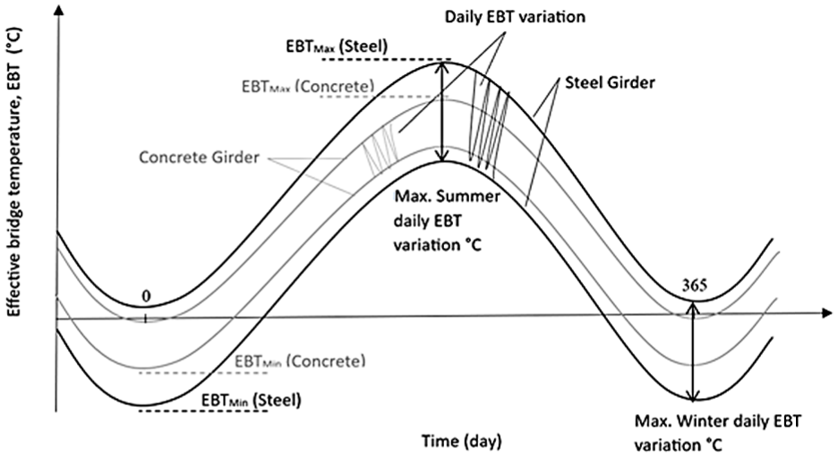
Graphical summary of effective bridge temperatures (EBTs) showing seasonal and daily variations.

Construction Temperature (CT)

Arsoy preferred the term “construction temperature” while Roeder used the term “installation temperature,” but both terms are the same, and they can be used interchangeably ( 16 , 18 ). CT may be defined for integral bridges as the EBT when the integral connection between the bridge deck and the abutment is made. The time of integral connection can be defined as the time when the connection is strong enough to handle thermal loadings and displacements, or when the interaction between the bridge and the soil begins. For jointed bridges, the CT is the EBT of the bridge immediately after the girders have been set on the bridge bearings.

Bridge Design Temperatures

Bridge design specifications state that provisions must account for stresses or movements arising from temperature variations or, more specifically, variations in EBTs. Fluctuations in temperature must be determined for each specific locality where a structure is erected and computed based on an assumed temperature at construction time by the following equations:

Δ T (+) = {EBT}_{\max} - CT

(2)

Δ T (-) = {EBT}_{\min} - CT

(3)

where

ΔT = design temperature,

CT = construction temperature,

EBT_max = the maximum extreme EBT expected during the lifespan of the bridge, and

EBT_min = the minimum extreme EBT expected during the lifespan of the bridge.

EBT_max and EBT_min differences are usually referred to as “design temperatures.” They are required to be known for estimating both expansion and contraction movements occurring within bridge girders.

Consideration of uniform temperature variations is common in different bridge design specifications which usually limit allowable design temperature variation (±ΔT) for a structure. These specifications sometimes provide a range from EBT_max to EBT_min. In such cases, the change in temperature is determined as the average value between the minimum and maximum design temperatures; that is, (EBT_max + EBT_min)/2. This procedure uses the change in design temperature (±ΔT) to determine the thermal displacement, regardless of the actual value of CT. In the U.S., AASHTO LRFD advises a temperature range for design (i.e., a maximum rise and fall) based on climate conditions and materials used in the superstructure ( 6 ). For example, many states in the northern region of the U.S. have minimum and maximum design temperatures of −34°C (−30°F) and 49°C (120°F) for a thermal range of 83°C (150°F) as per AASHTO LRFD design temperatures ( 13 ). The following tables present the evolution of design temperatures specified by AASHTO Standard Specifications 1996 and AASHTO LRFD for different years for steel bridges (Table 1) and concrete bridges (Table 2) ( 13 , 25 ).

Table 1.

Evolution of Design Temperatures (ΔT) for Steel Bridges in the U.S.

Bridge design specifications	Temperature (T) ranges for steel bridges
AASHTO Standard Specifications (1996) ( 25 )	Moderate climate: T_min−18°C (0°F) to T_max 49°C (120°F) Cold climate: T_min−34°C (−30°F) to T_max 49°C (120°F)
Massachusetts Highway Department Bridge Manual (1999) ( 26 )	ΔT_max+40°C (+72°F) ΔT_min−55°C (−99°F)
Many states in the northern region of the U.S., AASHTO LRFD (2010) ( 13 )	T _min−34°C (−30°F) to T_max 49°C (120°F)
AASHTO LRFD, Procedure B (2012) ( 27 )	Temperature range 69°C (125°F): ±ΔT = ±34°C (±62.5°F)
AASHTO LRFD (2015) ( 28 )	Temperature range 66°C (120°F): ±ΔT = ±33°C (±60°F)
AASHTO LRFD (2024) ( 6 )	Moderate climate: T_min−18°C (0°F) to T_max 49°C (120°F) Cold climate: T_min−34°C (−30°F) to T_max 49°C (120°F)

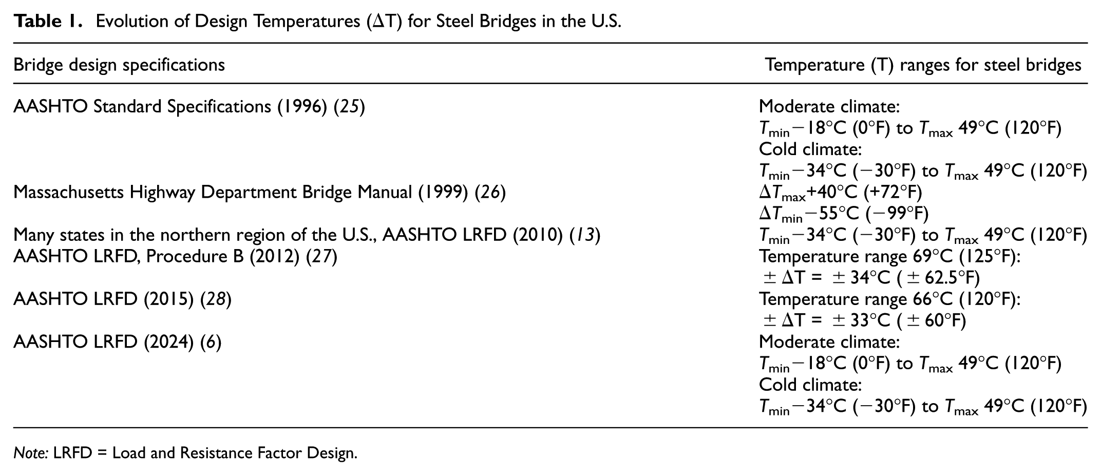
Note: LRFD = Load and Resistance Factor Design.

Table 2.

Evolution of Design Temperatures (ΔT) for Concrete Bridges in the U.S.

Bridge design specifications	Temperature (T) ranges for concrete bridges
AASHTO Standard Specifications (1996) ( 25 )	Moderate climate: ΔT_max = +17°C (+30°F) ΔT_min = −22°C (−40°F) Cold climate: ΔT_max = + 19°C (+35°F) ΔT_min = −25°C (−45°F)
AASHTO LRFD (2004) ( 29 )	Moderate climate: T_min−12°C (10°F) to T_max 27°C (80°F) Cold climate: T_min−18°C (0°F) to T_max 27°C (80°F)
AASHTO LRFD (2010), California ( 13 )	T _min−1°C (30°F) to T_max 46°C (115°F)
AASHTO LRFD (2010), Pennsylvania ( 13 )	T _min−12°C (10°F) to T_max 27°C (80°F)
AASHTO LRFD (2024), Procedure A ( 6 )	Moderate climate: T_min−12°C (10°F) to T_max 27°C (80°F) Cold climate: T_min−18°C (0°F) to T_max 27°C (80°F)

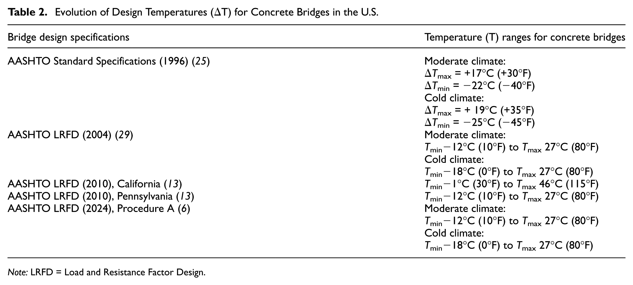
Note: LRFD = Load and Resistance Factor Design.

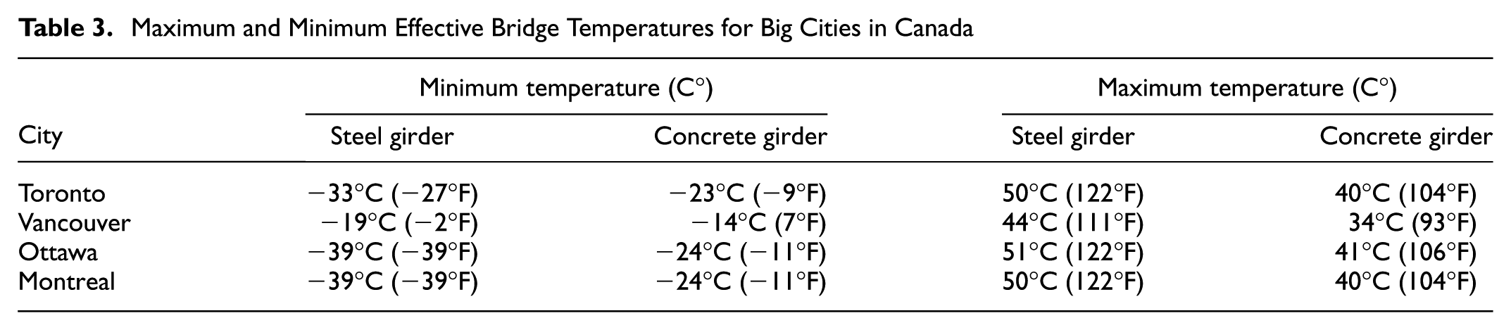
The Canadian Highway Bridge Design Code (CHBDC) by CSA (2019) specifies different temperature variations from those in the U.S. to be considered for different types of bridge ( 7 ). The minimum average temperatures used for steel and concrete bridges are regarded as 15°C (27°F) and 5°C (9°F), respectively, below the minimum daily mean temperature. Conversely, the maximum average temperatures for steel and concrete are considered as 25°C (45°F) and 10°C (18°F) above the maximum daily mean temperature, respectively. In cases where specific site data is unavailable, an effective CT of 15°C (60°F) is provided for both steel and concrete bridges. The maximum and minimum daily mean temperatures are extracted from the provided maps in CHBDC. Table 3 illustrates the maximum and minimum temperature design for four major cities in Canada, adapted from Nikravan ( 30 ).

Table 3.

Maximum and Minimum Effective Bridge Temperatures for Big Cities in Canada

City	Minimum temperature (C°)		Maximum temperature (C°)
City	Steel girder	Concrete girder	Steel girder	Concrete girder
Toronto	−33°C (−27°F)	−23°C (−9°F)	50°C (122°F)	40°C (104°F)
Vancouver	−19°C (−2°F)	−14°C (7°F)	44°C (111°F)	34°C (93°F)
Ottawa	−39°C (−39°F)	−24°C (−11°F)	51°C (122°F)	41°C (106°F)
Montreal	−39°C (−39°F)	−24°C (−11°F)	50°C (122°F)	40°C (104°F)

According to Eurocode CEN guidelines, temperature variation in bridges include defining uniform temperature components for both expansion (ΔT_N,exp) and contraction (ΔT_N,con) ( 8 ). These components can be determined as follows: $Δ T_{N, \exp} = EB T_{e . \max} - T_{0}$ , $Δ T_{N, con} = T_{0} - {EBT}_{e . \min}$ . The overall range of the uniform bridge temperature component can be determined as follows:

Δ T_{N} = {EBT}_{e . \max} - EB T_{e . \min}

(4)

where

EBT_e.max = the maximum uniform bridge temperature component, and

EBT_e.min = the minimum uniform bridge temperature components, (also defined as the EBT: these values are derived from the minimum and maximum SATs).

Meanwhile,T₀ refers to the initial temperature of the bridge, also defined as the CT. It ideally reflects the temperature of a structural element during its specific restraint stage, commonly referred to as the “completion phase.” In cases where the initial temperature is unpredictable, the average temperature during the construction period is considered instead. The initial temperature value may be specified for an individual project or in standard codes and specifications. In the absence of available information, the initial temperature may be assumed as 10°C. In situations where uncertainty exists about the bridge’s sensitivity to the initial temperature, it is advisable to consider both a lower and upper limit for expected initial temperature.

Proposed Approach for Construction Temperature (CT) Specification

Maximum thermal changes in IABs would exceed specified design temperatures depending on actual variability of CT, as further discussed in the following subsection. As a solution, this study proposes that there is a rationale for considering CT as a controllable design parameter. Recommending a specific range for CT [CT_min, CT_max] during design phase and implementing it during construction phase may offer a solution and significantly reduce uncertainty related to adverse effects of actual CT. Consideration of CT as a design parameter within a defined and implemented range introduces a new perspective on resolving challenges associated with IABs.

Discussion on Current Construction Temperature (CT) Considerations

CT is a future event and an unknown factor during the design process, needing assumptions. However, some bridge design specifications do not offer clear guidance for assuming CT. Instead, they suggest using a temperature range (i.e., design temperatures) to compute the expected maximum thermal displacement of bridge superstructure, regardless of the actual value of CT. Consequently, CT assumed by design specifications may be indirectly inferred from those design temperatures (ΔT), and it can be mathematically represented as follows:

CT = ({EBT}_{\max} + {EBT}_{\min}) / 2 \pm Δ T .

(5)

where

EBT_max = the maximum expected temperature within the specified range,

EBT_min = the minimum expected temperature within the specified range, and

ΔT (±) = the expected variation in temperature (design temperatures) from the initial CT in contrast to other specifications which provide recommendations for CT.

In general, bridge design specifications typically do not establish specific limitations for a lower or upper bound for CT for bridges.

This subsection discusses how the consideration of CT varies across different bridge design specifications in the U.S., Canada, and Europe. In accordance with AASHTO LRFD, steel bridges designed for moderate climates are intended for extreme average bridge temperatures ranging from −18°C (0°F) to +49°C (120°F) ( 6 ). Calculating the temperature variation as the mean value (EBT_av) between the minimum and maximum EBTs [EBT_av = (EBT_max + EBT_min)/2] results in a range of ±33.5°C (±60°F). Given that the total temperature ranges between the extreme EBTs are 67°C (120°F), the implied CT derived from AASHTO’s specifications would be [CT = EBT_av ± ΔT] at 15.5°C (60°F). For concrete bridges in moderate climates, the specifications suggest a rise in temperature ΔT (+) of +16.7°C (+30°F) and a fall in temperature of ΔT (–) of −22.2°C (−40°F). The total temperature range considering these variations (ΔT (+) + ΔT (–)) amounts to 38.9°C (70°F). However, assuming the CT for the concrete bridge to be the same as that for steel bridges, which is 15.5°C (60°F), would align with the AASHTO implication. The visual representation in Figure 2 illustrates the seasonal and daily variations in EBTs for both steel and concrete decks within one yearly thermal cycle.

Figure 2.

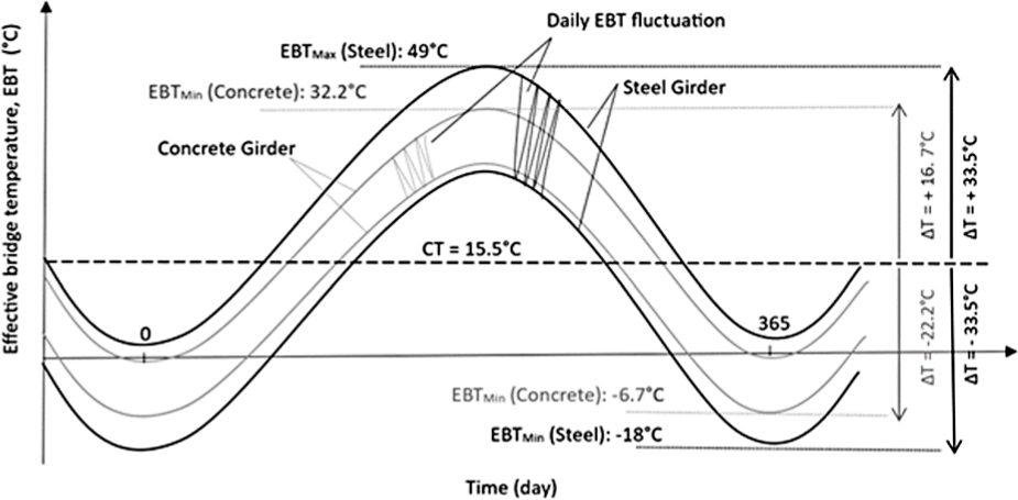
Variations in effective bridge temperatures (EBTs) for both steel and concrete decks within one thermal cycle of a year considering an implied construction temperature (CT) of 60°F (15.5°C) as derived from AASHTO’s specifications.

The potential deviation between implied CTs derived from AASHTO’s specifications and actual variability in CT might result in temperature changes (±ΔT) that exceed design temperature variations specified by AASHTO. In the context of this discussion, considering a pragmatic range of CT variance spanning from −1.1°C (30°F) to 32.2°C (90°F), the maximum thermal differentials observed were ±50°C (±90°F) for steel, and +45°C (+80°F) and −50°C (−90°F) for concrete, as graphically represented in Figure 3. It is noteworthy that these variations exceed the prescribed design temperatures outlined by AASHTO specifications.

Figure 3.

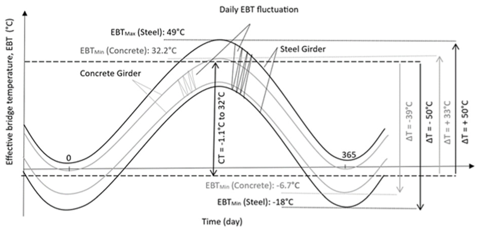
Possible real extreme variations in effective bridge temperatures (EBTs) for both steel and concrete decks within one thermal cycle of a year considering range of construction temperatures (CTs) spanning from −1.1°C (30°F) to 32.2°C (90°F).

In general, different states in the U.S. adopt varying criteria and procedures concerning the consideration of CTs. Iowa Department of Transportation recommends taking into account temperature variations during construction by applying setting factors of 1.50 for precast pre-stressed concrete bridges and 1.33 for continuous welded plate girder bridges. These factors aim to increase the calculated thermal movement for CTs ranging from −4°C to 24°C (25°F to 75°F) ( 31 ).

According to CHBDC, the observation that was previously considered in AASHTO specifications remains applicable, as CHBDC adopts a specific CT value of 15°C in the absence of site-specific data for both steel and concrete bridges. Considering the realistic variability in CT, as demonstrated in Figure 3, the resulting maximum thermal changes observed in both steel and concrete bridges would still possibly exceed the specified design temperatures.

According to Eurocode, recommendations are provided to directly assume CT, which is defined as the temperature of the element at the relevant stage of its restraint (completion). In cases where CT is unpredictable, the average temperature during the construction period is considered instead. This initial temperature value may be specified in the National annex or within a particular project. In the absence of available information, CT may be assumed as 10°C. In situations where uncertainty exists about the bridge’s sensitivity to CT, it is advisable to consider both a lower and upper bound representing the expected interval for CT. Eurocode takes into account the realistic variability in CT and its potential impact on a bridge’s performance in scenarios where uncertainty exists about the bridge’s sensitivity to CT.

Proposed Mathematical Model

Determination of an exact temperature range for construction is complicated because of variable environmental conditions and project-specific factors. This study examines the feasibility of defining a CT range using the mathematical model of Arsoy for defining diurnal and seasonal fluctuating of temperatures ( 18 ). This model accounts for temperature difference patterns encompassing both seasonal and daily cycles of EBTs at any location where meteorological data are available. Managing CTs within these defined ranges enables accurate predictions of induced thermal displacement variations over time and associated internal forces in bridge elements affected by thermal loads.

As discussed earlier, the primary factors that influence EBT include diurnal temperature variations, solar variation, wind speed, precipitation, and thermal properties and geometry of structures. The actual value of EBT is a result of heat transfer from/to the surrounding environment of a bridge. As known well in physics, while heat is the thermal kinetic energy transferred from one point to another, temperature is the average thermal kinetic energy within a material. This means that the temperature is a rough indication of stored energy within a material and that heat transfer is caused by a difference in temperature between adjacent points. So, when SAT increases, heat is transferred to the bridge, causing an increase in EBT. The reverse is also true when SAT decreases—heat is transferred from the bridge to the surroundings, causing a decrease in EBT. Solar radiation is a form of electromagnetic energy transfer through infrared radiation emanating from the sun. As a result, solar radiation transfers additional heat during non-cloudy day times to a bridge, and tend to create an increase in EBT, in addition to that which arises from SAT. Clouds, any shade, and non-daylight times cause the effect of solar radiation immediately to go away, as if an infrared heater were switched off. Wind, precipitation, and evaporation may remove heat from the bridge to the surroundings.

From a theoretical point of view, all factors discussed above must be satisfied for real-time analysis. However, a bridge is designed to serve for a long time; as a result, one would need to focus on seasonal trends. As also discussed earlier, there is also a time lag between SAT and other heat transfer factors to affect EBT through heat transfer. Thermal properties and the geometric properties of the bridges also play a role. Additionally, SAT, EBT, and CT are all future variables, and they may vary significantly from one season to another. The purpose is not to model the exact values, but the main trends based on statistical evaluations of historical temperature data.

Considering the complexity and purpose of this study, the proposed model assumes that CT mimics the variation of SAT and, therefore, the model is built on SAT. As a result, the proposed model relies on expected maximum and minimum SATs, as well as average daily temperature variations derived through statistical analyses of historical data over a specific timeframe, such as 40 years. It also includes the difference between the limit values of the EBTs, aligned with the expected maximum and minimum SATs or less, depending on the bridge type. Moreover, the model takes into consideration the seasonal cycles of EBTs, along with daily fluctuations, resembling a sine function in their time-dependent variations.

During construction, CT can be any value from as high as EBT_max and to as low as EBT_min; therefore, it can be defined that CT for the seasonal variation can be represented as follows:

CT (t) = {CT}_{\min} + {CT}_{amp} [1 + (\sin (\frac{2 π}{365} (t + t_{0})))]

(6)

{CT}_{amp} = \frac{{CT}_{\max} - {CT}_{\min}}{2}

(7)

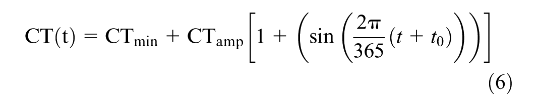
where

t = time in days starting at beginning of the calendar year (00:00 on January 1^st), and

t ₀ = time shift in days to define the initial value of CT (t = 0) at January 1^st for the particular bridge location (considered because a sine function yields the lowest value at ¾ of its period; e.g., consider a location where the lowest temperature is expected at the beginning of February, there will be a time shift of t₀ = ¾ x 365 − 30 = 244 days).

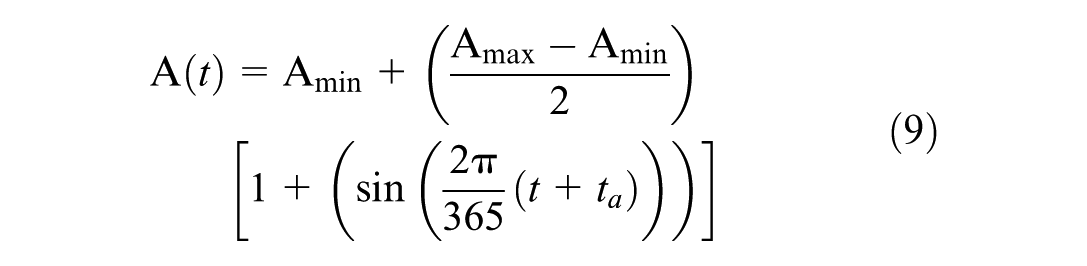
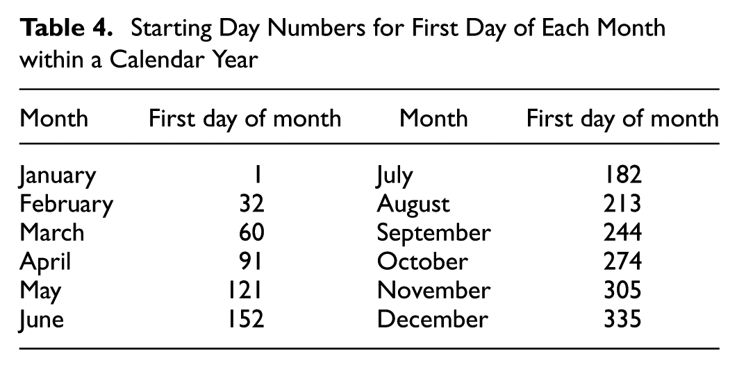
Table 4 can be used to standardize the starting day of each month in a calendar year. If the daily variation is included, the above equation becomes:

\begin{matrix} CT (t) = ({CT}_{\min} + A (t)) \\ + ({CT}_{amp} - A (t)) [1 + (\sin (\frac{2 π}{365} (t + t_{0})))] \\ + A (t) \sin (2 π (t + t_{d})) \end{matrix}

(8)

where

A(t) = the time-dependent daily temperature fluctuation (defined below in Equation 9),

A_max = the maximum value of A(t) fluctuation (equal to half the maximum daily difference in EBT for a given year),

A_min = the minimum value of A(t) fluctuation (equal to half the daily difference in EBT for a given year),

(in other words, A(t) varies linearly between A_max and A_min as well as A_min to A_max during a whole year and models the variation of diurnal temperature range throughout the whole year),

t _d = hourly phase shift in unit of days between 0 and 1 (set for initiating time of a day) (to define the initial value of A(t = 0) at particular location; i.e., t_d = 6/24 = 0.25 if A_min is observed at 06:00 for a given day), and

t _a = phase shift (days) to tune the daily variation parameter A to match A_max and A_min values at their corresponding calendar days in the sine function.

Consider a location where the highest daily temperature fluctuation is expected at the beginning of March and the lowest temperature is expected at the beginning of February, there will be a time shift of t₀ = ¼ x 365 − 30 = 61 days because the maximum value of a sine function takes place at ¼ of its period and there is a nominal 30-day difference between March and February. A numerical example (presented later) provides further explanations about t₀, t_d, and t_a.

\begin{matrix} A (t) = A_{\min} + (\frac{A_{\max} - A_{\min}}{2}) \\ [1 + (\sin (\frac{2 π}{365} (t + t_{a})))] \end{matrix}

(9)

In applying this model, CT values can be estimated from historical SATs by observing that it is more reasonable to consider the most likely low and high EBTs rather than using the extreme values (i.e., EBT_max and EBT_min). Necessary parameters in the above equations can be easily obtained from meteorological data of record highs and lows and from mean highs-lows. If CT is to be selected as a single value equal to the average of EBT_max and EBT_min, it would be ideal for achieving symmetrical bridge movements during expansion and contraction cycles, but construction scheduling becomes severely restrictive. On the contrary, if CT is set as a range of [EBT_max, EBT_min], construction scheduling becomes almost unrestricted, but bridge movements may become significantly asymmetrical and unwanted. To define the low and high of CTs without adversely affecting the construction scheduling, it is proposed to base it to a value between the recorded peaks and the average means.

Table 4.

Starting Day Numbers for First Day of Each Month within a Calendar Year

Month	First day of month	Month	First day of month
January	1	July	182
February	32	August	213
March	60	September	244
April	91	October	274
May	121	November	305
June	152	December	335

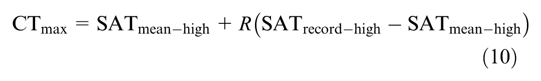
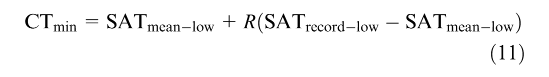
The adverse effect of a selected range for CT on construction scheduling can be defined by assuming temperature variations for highs and lows are independent variables and each is normally distributed. An additional assumption is that record high and record low values are three standard deviations (3σ) away from their mean high and mean low values, respectively. These assumptions allow quantifying the standard deviation, σ, as one third of the difference between the mean and record values for highs and lows separately, and probability calculations become simple using the normal distribution table. A parameter R between 0 and 1 can be introduced to set the upper and lower limit of daily CT values by considering the same fraction of higher ranges (SAT_record-high–SAT_mean-high) and lower ranges (SAT_record-low–SAT_mean-low). As a result, probability calculations become simpler because the multiplier of σ can be quantified as 3R. If R is taken as 0, the daily range of CT fluctuates from mean-low to mean-high and the multiplier of σ becomes equal to 0 × 3 = 0 (mean values) when using the normal distribution table. When R is taken as 1, the daily range of CT varies from record-low to record-high and the standard deviation multiplier becomes equal to 1 × 3 = 3 (3σ away from mean values) when using the normal distribution table.

Daily variable values of potential candidates for the CT range of [CT_min, CT_max] can be stated using SAT_record-high and SAT_mean-high for CT_max, using SAT_record-low and SAT_mean-low for CT_min, and the parameter R between 0 and 1, as follows:

{CT}_{\max} = {SAT}_{mean - high} + R ({SAT}_{record - high} - {SAT}_{mean - high})

(10)

{CT}_{\min} = {SAT}_{mean - low} + R ({SAT}_{record - low} - {SAT}_{mean - low})

(11)

Daily variation parameter A_max is quantified as the half of the maximum daily difference of CT_max − CT_min, and A_min is quantified as the half of the minimum daily difference of CT_max − CT_min.

The adverse effect of any selected range of CT on construction scheduling will be equal to the combined probabilities of exceedance of CT_min and CT_max. Table 5 presents such effects for selected R values as combined probability of SAT constraining bridge construction for each given time unit, assuming temperature variations for highs and lows are independent variables and each is normally distributed, as discussed earlier. Data in Table 5 are regenerated using normal distribution tables and the combined probability rule, and it suggests that opting for a value for CT with R = ½ corresponding to 50% of the difference between the average mean and the peak value, and the same for the lows, would be the best case for restrictiveness of construction scheduling with an expected adverse probability of 0.0044 (0.44%). Calculations steps for R = ½ are provided for familiarity, as follows. When R is ½, the multiplier of σ becomes 0.5 × 3 = 1.5, corresponding to the case that CT_max and CT_min values are 1.5σ away from their mean values. Subsequently, from the normal distribution table, the probability of exceedance for 1.5σ for each of CT_max and CT_min can be obtained as 0.0668. Using the combined probability rule, the final value of the expected combined adverse probability of exceedance [CT_max, CT_min] for R = ½ becomes 0.0668 × 0.0668 = 0.0044 or 0.44%. If a tighter range is desired with slightly increased adverse effect, it can be specified with smaller R values.

Table 5.

Simplified Probabilistic Evaluation of Adverse Construction Effect of Selected [CT_min, CT_max] for Each Time Unit

R	P (not meeting CT_min)	P (not meeting CT_max)	P (combined)
0	0.5000	0.5000	0.2500
1/5	0.2743	0.2743	0.0752
1/4	0.2266	0.2266	0.0513
1/3	0.1357	0.1357	0.0184
1/2	0.0668	0.0668	0.0044
1	0.0113	0.0113	0.0001

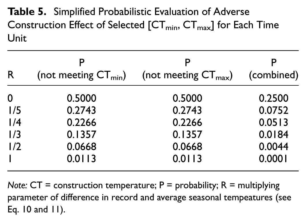
Note: CT = construction temperature; P = probability; R = multiplying parameter of difference in record and average seasonal tempeatures (see Eq. 10 and 11).

Meteorological data for SAT is usually provided monthly (i.e., time unit). Accordingly, potential candidates for CT can be defined using Equations 6–11, with CT_max selected from the hottest month and CT_min selected from the coolest month for the desired construction effect. Figure 4 provides a schematic illustration of the expected CT variation throughout a year, along with extreme EBT seasonal variation. It is recommended that the final decision for the CT range [CT_f.min, CT_f.max] should be made for the bridge designer by examining the seasonal variation and defining a range that can be achievable throughout the year, such as that shown also in Figure 4. Please note that the range [CT_f.min, CT_f.max] shown as a gray area in the figure, is for illustrative purposes to help visualize the final range adopted with respect to the expected high and low values of CT candidates throughout a season. The bridge designer should set CT_f.min lower than high CT values observed in winter times, and CT_f.max higher than low CT values observed in summer times. Additionally, [CT_f.min, CT_f.max] should define a symmetric band as narrow as possible around the seasonal middle value of (EBT_max + EBT_min)/2.

Figure 4.

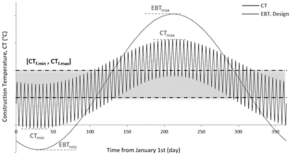
Daily schematic variations of construction temperature (CT) for selected adverse probability in within a year and selected single range.

It should be noted that a single range [CT_min, CT_max] defined for the whole year will have a higher probability of adverse effects on construction scheduling than those discussed earlier (see Table 5). If desired, calculation of the total probability of adverse effects on construction scheduling can be made by calculating the combined probability of adverse effects for each day for the final single range set for CT, and summing the probabilities of adverse effects. However, this can be tedious, and an average bridge designer would not prefer to do this, but it can be implemented if construction scheduling is very important. On the other hand, it should not be forgotten that the main goal is to obtain symmetrical bridge movements, which is achievable only with as narrow a CT range as possible. Therefore, the final range for CT should be decided for each locality by applying the proposed methodology with the engineering judgement of the designer. Additionally, construction scheduling can be managed ahead of time by planning the integral connection task for fall or spring season to reduce restrictiveness. Moreover, potential adverse effects on construction scheduling can be mitigated further by planning the relevant tasks for late nights in summer and daytime in winter.

Numerical Application

A numerical example is presented below for familiarization of the proposed approach for a hypothetical bridge to be constructed in Istanbul. The statistical evaluations of historical data spanning 72 years are available and derived from the T.C. Ministry of Environment, Urbanization, and Climate Change (General Directorate of Meteorology) of Turkey. Table 6 provides the mean high, mean low, average mean, and maximum and minimum values of SATs recorded between 1950 and 2022 for each month in Istanbul. The maximum and minimum temperatures recorded over a span of 72 years are 40.6°C in July and −9°C in February, respectively. In consideration of the extreme environmental conditions that the bridge may endure throughout its operational duration, these peak values will be adopted as design parameters.

Table 6.

Temperature Variation Patterns in Istanbul (1950–2022) (Temperatures in °C)

SA Category	Jan	Feb	Mar	Apr	May	Jun	Jul	Aug	Sep	Oct	Nov	Dec
SAT_mean-high	9.5	10.2	12.2	17.3	22.3	26.9	29.5	29.6	25.8	20.6	16.0	11.7
SAT_mean-low	4.1	4.2	5.4	9.2	13.6	18	20.4	20.7	17.6	13.7	9.8	6.4
SAT_mean-avg	6.7	6.9	8.4	12.8	17.6	22.2	24.6	24.6	21.1	16.6	12.5	8.9
SAT_record-high	22.4	23.4	28.6	33.3	36.4	38.9	40.6	40.1	39.6	33.5	27.2	25.0
SAT_record-low	−6.8	−9.0	−5.6	0.2	4.8	9.8	13.6	14.3	7.7	2.5	−2.0	−4.2

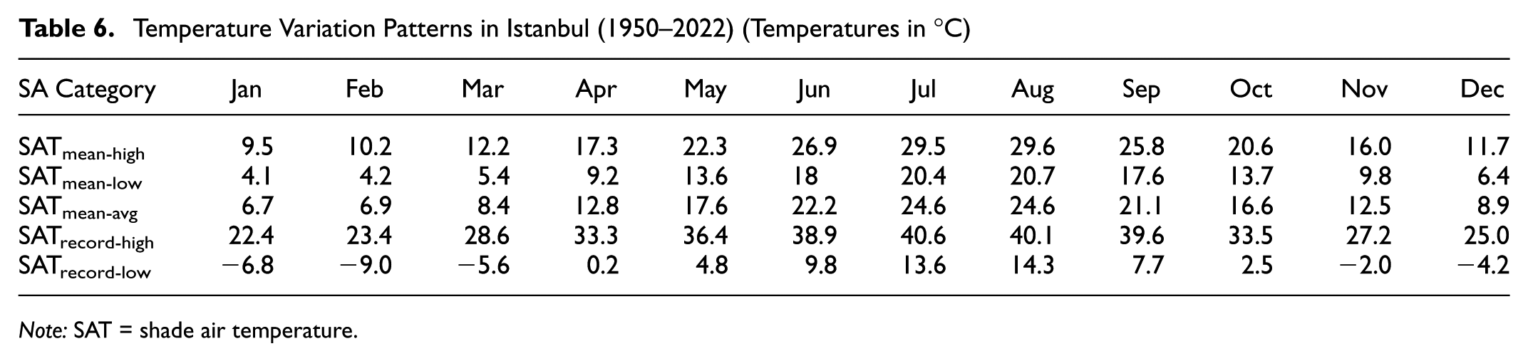
Note: SAT = shade air temperature.

Given that the meteorological data for SAT is provided on a monthly basis, the range of potential CT values [CT_min, CT_max] is determined for each month using Equations 10 and 11. The recommended value of R of ½ has been used. The potential candidates for the CT values [CT_min, CT_max] and the daily variation parameters A_max and A_min, to be utilized in the proposed model using Equations 6–9, will be selected based on the proposed methodology. CT_max is determined from the hottest month, observed in July, with a recorded value of 35.1°C, while CT_min is derived from the coolest month, observed in January, with a recorded value of −2.4°C. Consequently, the amplitude of the EBT, CT_amp, is calculated at 18.7°C. Concerning the daily variation parameters, A_max represents half of the maximum difference between CT_max (from Equation 10, 17.3 − 0.5(33.3 − 17.3) = 25.3) and CT_min (from Equation 11, 9.2 − 0.5(0.2 − 9.2) = 4.7) observed in April, which is 20.6°C (25.3 − 4.7). Therefore, A_max is equal to 10.3°C (20.6/2). A_min, on the other hand, represents half of the minimum difference between CT_max and CT_min observed in December, which is 17.3°C. Thus, A_min is equal to 8.3°C.

The sine function, as described in Equation 8, initiates from the average value of the range if no adjustment for time shift t₀ were made and the sine function would yield its minimum value at ¾ of its period corresponding to t = 274. However, in the example, t = 0 corresponds to January 1^st and the lowest temperature is seen at the beginning of February. To align the first value of the function with the temperature on January 1^st, a time shift of 244 days (274 − 30) is required. This adjustment ensures that the function aligns accurately with the temperature data on the specified date, such that t starts from first calendar day and the lowest temperature is seen 30 days after the initiation of t. Therefore, t₀ = 244 is deemed appropriate. Disregarding hourly temperature variations, t_d = 0 is assigned. If one assumed the lowest temperature for a given day were at 04:00 in the morning, then t_d = 1/6 = (4/24) would have been chosen. As the peak variation in daily temperatures occurs halfway through a period (183 days) from the sine function’s beginning when t₀ = 244, the value of t_a is set at 61 days after the initiation day (t_a = 244 − 183 = 61), considering the starting value of the sine function has a time shift of 244 days. The proposed model can be utilized to estimate time-dependent temperature variation as follows:

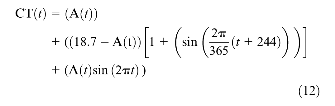
\begin{matrix} CT (t) = (A (t)) \\ + ((18.7 - A (t)) [1 + (\sin (\frac{2 π}{365} (t + 244)))] \\ + (A (t) \sin (2 π t)) \end{matrix}

(12)

The parameter for daily temperature difference is presented as follows:

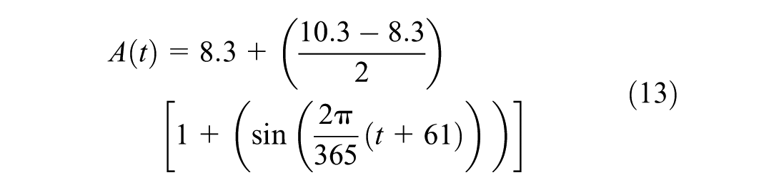
\begin{matrix} A (t) = 8.3 + (\frac{10.3 - 8.3}{2}) \\ [1 + (\sin (\frac{2 π}{365} (t + 61)))] \end{matrix}

(13)

Figure 5 displays the graphical variation of time-dependent temperature changes for CT. To enhance graph clarity, every fifth daily cycle is presented (i.e., sine function) along with the seasonal EBT variation (dotted line). The sine function in the figure shows the expected daily and seasonal variations of CTs. Consequently, based on this mathematical model, the recommended CT range can be defined to remain applicable throughout the year. The ideal CT for this location is EBT_av = (EBT_max + EBT_min)/2 which is (40.6 + (−9.0))/2 = 15.8°C for perfect symmetrical variation of expansion and contraction cycles of the bridge. However, mandating 15.8°C as the CT for this bridge would be severely restrictive for construction, as discussed earlier.

Figure 5.

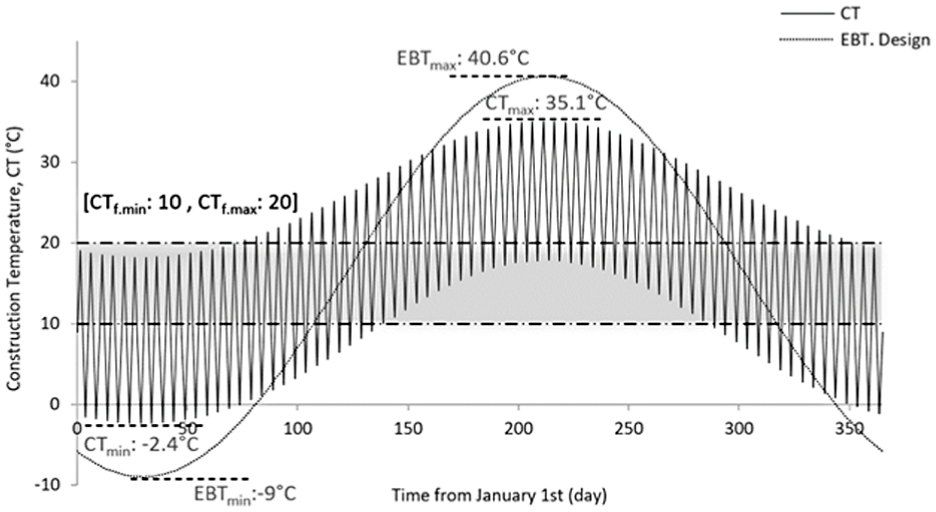
Daily variations of construction temperature (CT) within a year and selected single range for the numerical example.

The bridge designer should set a band around the middle value of 15.8°C such that CT_f.min is lower than the high CT values observed in winter times and CT_f.max is higher than the low CT values observed in summer times (Figure 5). For the sake of simplicity of the example, if the ideal temperature is rounded down to 15°C and a symmetrical band of ±5°C is deemed appropriate, a mandatory CT range can be established as 15°C ± 5°C or [10°C, 20°C]. During winter, the desired CT could be set during the daytime, while in summer, it could be established during nighttime. The suggested range using engineering judgement, for this example, is [CT_f.min = 10°C, CT_f.max = 20°C].

It is recommended for this example that a CT range of [10°C, 20°C] is enforced as a mandatory specification during construction, and the expansion and contraction cycles of the bridge are designed accordingly. In the design, a temperature rise of EBT_max – CT_f.min and a temperature fall of CT_f.max – EBT_min, which corresponds to about ±30°C, should be adopted.

Conclusions

This paper provides a novel perspective on resolving challenges related to the limited length of IABs, contributing to improved structural integrity and performance. More specifically, this study proposes mandatory CT specifications set during the design stage for bridge contractors to satisfy during the construction stage for IABs. Important conclusions withdrawn from this study are as follows:

Current practice does not mandate an initial CT range during construction, leading to potential mismatches between the assumptions made during design and actual field construction conditions.

This study proposes a practical and easily applicable methodology for setting and mandating CT as a specification to be jointly implemented during both in design and in construction for IABs.

The proposed methodology requires reviewing historical temperature data relevant to the specific locality of the bridge to be erected.

The output of the proposed method is a tight range for CT, applicable on most days without significant adverse effects in construction scheduling.

Attaching CT as a criterion into design protocols may result in enhanced predictions of expansion/contraction thermal displacement patterns and internal forces within IABs.

Optimizing and mandating CT also aids in mitigating adverse effects of thermal loading across various design scenarios.

Real-case advantages of the proposed mathematical model in strain/stress/displacements may vary from those discussed in this study. Field practitioners are encouraged to test the benefits of the proposed model.

Collaboration among all participants from designers to field implementers is important because of challenges in specifying an exact temperature range under varying environmental conditions and project-specific factors.

Valuable insights and actionable recommendations may be achieved to enhance the reliability, longevity, and efficiency of IABs through overall performance improvements.

The proposed methodology can be expanded to define CT for girder placement in jointed bridges if symmetrical displacement accommodation is required. The methodology presented can also be used for other structures where thermal displacements are of concern.

Footnotes

Acknowledgements

The infrastructure of the information resources of Kocaeli University, Turkey, has been used in conducting this research and is greatly acknowledged. We sincerely appreciate the constructive comments and criticisms raised and offered by the anonymous reviewers.

Author Contributions

The authors confirm contribution to the paper as follows: study conception and design: S. Arsoy; data collection: H. Rifai; analysis and interpretation of results: H. Rifai, S. Arsoy; draft manuscript preparation: H. Rifai, S. Arsoy. All authors reviewed the results and approved the final version of the manuscript.

Declaration of Conflicting Interests

The authors declared no potential conflicts of interest with respect to the research, authorship, and/or publication of this article.

Funding

The authors received no financial support for the research, authorship, and/or publication of this article.

ORCID iD

Sami Arsoy

Data Accessibility Statement

All data, models, or code generated or used during the study are included in the manuscript.

References

Kim

Laman

J. A.

Seven-Year Field Monitoring of Four Integral Abutment Bridges. Journal of Performance of Constructed Facilities, Vol. 26, No. 1, 2012, pp. 54–64. https://ascelibrary.org/doi/abs/10.1061/(ASCE)CF.1943-5509.0000250.

Peric

Mietic

Shah

B. R.

Esmaeily

Wang

Thermally Induced Soil Structure Interaction in the Existing Integral Bridge. Engineering Structures, Vol. 106, 2016, pp. 484–494. https://www-sciencedirect-com-443.web.bisu.edu.cn/science/article/pii/S0141029615006665.

Kim

Laman

J. A.

Integral Abutment Bridge Response Under Thermal Loading. Engineering Structures, Vol. 32, No. 6, 2010, pp. 1495–1508. https://www-sciencedirect-com-443.web.bisu.edu.cn/science/article/pii/S0141029610000052.

Murphy

Yarnold

Temperature-Driven Structural Identification of a Steel Girder Bridge with an Integral Abutment. Engineering Structures, Vol. 155, 2018, pp. 209–221. https://www-sciencedirect-com-443.web.bisu.edu.cn/science/article/pii/S0141029617316644.

Lee

Jeong

Kim

Buckling Behavior of Steel Girder in Integral Abutment Bridges Under Thermal Loadings in Summer Season During Deck Replacement. International Journal of Steel Structure, Vol. 16, 2016, pp. 1071–1082. https://link-springer-com-443.web.bisu.edu.cn/article/10.1007/s13296-016-0023-x.

AASHTO LRFD Bridge Design Specifications . AASHTO LRFD 10th ed. American Association of State Highway and Transportation Officials, Washington, D.C., 2024.

Canadian Standards Association. Canadian Highway Bridge Design Code, CSA S6:19. Toronto, ON, Canada, November 2019.

European Committee for Standardization. Eurocode 1: Actions on Structures, EN 1991-5 Part 1.5: General Actions - Thermal Actions. Brussels, Belgium, 2003.

Girton

D. D.

Hawkinson

T. R.

Greimann

L. F.

Validation of Design Recommendations for Integral-Abutment Piles. Journal of Structural Engineering, Vol. 117, No. 7, 1991, pp. 2117–2134. https://ascelibrary.org/doi/abs/10.1061/(ASCE)0733-9445(1991)117:7(2117).

10.

AASHTO Standard Specifications for Highway Bridges, 13th ed. American Association of State Highway and Transportation Officials, Washington. D.C., 1983.

11.

Huang

Shield

C. K.

French

C. W.

Behavior of Concrete Integral Abutment Bridges. Report, No. 2004-43. Minnesota Department of Transportation, Minneapolis, 2004.

12.

AASHTO LRFD Bridge Design Specifications. American Association of State Highway and Transportation Officials, Washington, D.C., 2002.

13.

AASHTO LRFD Bridge Design Specifications, 5th ed. American Association of State Highway and Transportation Officials, Washington, D.C., 2010.

14.

Schlögl

Widhalm

Avian

Comprehensive Time-Series Analysis of Bridge Deformation Using Differential Satellite Radar Interferometry Based on Sentinel-1. ISPRS Journal of Photogrammetry and Remote Sensing, Vol. 172, 2021, pp. 132–146. https://doi.org/10.1016/j.isprsjprs.2020.12.001.

15.

Mirko Calo

Ruggieri

Nettis

Uva

A MTInSAR-Based Early Warning System to Appraise Deformations in Simply Supported Concrete Girder Bridges. Structural Control and Health Monitoring, Vol. 2024, 2024, p. 8978782. https://doi.org/10.1155/2024/8978782.

16.

Roeder

C. W.

Proposed Design Method for Thermal Bridge Movements. Journal of Bridge Engineering, Vol. 8, No. 1, 2003, pp. 12–19. https://ascelibrary.org/doi/abs/10.1061/(ASCE)1084-0702(2003)8:1(12).

17.

Lock

Integral Bridge Abutments. Report, No. CUED/D-SOILS/TR320. University of Cambridge, Department of Engineering. London, 2002.

18.

Arsoy

Proposed Mathematical Model for Daily and Seasonal Thermal Bridge Displacements. Transportation Research Record: Journal of the Transportation Research Board, 2008. 2050: 3–12.

19.

Quinn

Civjan

Parametric Study on Effects of Pile Orientation in Integral Abutment Bridges. Journal of Bridge Engineering, Vol. 22, No. 4, 2016, p. 04016132. https://ascelibrary.org/doi/abs/10.1061/(ASCE)BE.1943-5592.0000952.

20.

Boley

B. A.

Weiner

J. H.

Theory of Thermal Stress. Wiley, New York, NY, 1960.

21.

England

G. L.

Tsang

N. C.

Bush

D. I.

Integral Bridges: A Fundamental Approach to the Time–Temperature Loading Problem. Thomas Telford, London, 2000.

22.

Emerson

The Calculation of the Distribution of Temperature in Bridges. Transport and Road Research Laboratory (TRRL), Report, No. 561. Wokingham, Berkshire, 1973.

23.

Emerson

Temperature Differences: Basis of Design Requirements. Transport and Road Research Laboratory (TRRL), Report, No. 765. Wokingham, Berkshire, 1977.

24.

Moorty

Roeder

C. W.

Temperature-Dependent Bridge Movements. Journal of Structural Engineering, Vol. 118, No. 4, 1992, pp. 1090–1105. https://ascelibrary.org/doi/abs/10.1061/(ASCE)0733-9445(1992)118:4(1090).

25.

AASHTO Standard Specifications for Highway Bridges, 16th ed. American Association of State Highway and Transportation Officials, Washington. D.C., 1996.

26.

Mass Highway Bridge Manual. Design Guidelines and Standard. Details for Integral Abutment Bridges. Massachusetts Highway Department, Boston, MA, 1999.

27.

AASHTO LRFD Bridge Design Specifications, 6th ed. American Association of State Highway and Transportation Officials, Washington, D.C., 2012.

28.

AASHTO LRFD Bridge Design Specifications, 7th ed. American Association of State Highway and Transportation Officials, Washington, D.C., 2015.

29.

AASHTO LRFD Bridge Construction Specifications, 2nd ed. American Association of State Highway and Transportation Officials, Washington, D.C., 2004.

30.

Nikravan

Structural Design Issues for Integral Abutment. PhD thesis. Ryerson University, Toronto, Ontario, Canada, 2013. https://rshare.library.torontomu.ca/ndownloader/files/28127607.

31.

Tabatabai

Magbool

Bahumdain

Criteria and Practices of Various States for the Design of Jointless and Integral Abutment Bridges. Proc., Third International Workshop on Jointless Bridges, UWM Digital Commons, Seattle, D.C., 2017. https://dc.uwm.edu/cee_facart/9/.