Determinants of External Indebtedness in Heavily Indebted Poor Countries: What Macroeconomic and Socio-Economic Factors Matter?

Abstract

This study specifically examined whether macroeconomic and socio-economic factors such as corruption, foreign aid, government expenditure, external reserve, population growth, economic growth, and unemployment rate matter in increasing or reducing the level of external indebtedness in heavily indebted poor countries (HIPCs). Both static panel data and panel fully modified ordinary least squares (OLS) estimation techniques were employed. Using panel data set of all the 39 HIPCs covering period of 1996 to 2018, we found out that the factors that matter in heightening the intake of external debt are high rate of corruption that leads to mismanagement of public funds, high dependency on foreign aids, increase in government expenditure, population growth, and unemployment rate. However, external reserve and gross domestic product (GDP) has a reducing effect on their external indebtedness. In terms of causal relationship, only corruption, population growth, and GDP have a causal relationship with external debt, while other variables exhibited a zero causal relationship with external debt.

JEL Classifications: F34, E6, E24

Keywords

external indebtedness macroeconomic factors socio-economic factors heavily indebted poor countries

Introduction

Developing countries most especially the heavily indebted poor countries (HIPCs) are indeed characterized by low level of investment and economic growth, low external reserves, high level of unemployment, increasing government expenditure that often results to budget deficit, a rapidly growing population that increases much faster than the available resources, high level of corruption that leads to mismanagement of public funds and high poverty level and hence resort to borrowing from external sources to combat these economic problems.

HIPCs have continued to experience difficulties meeting their external debt service obligations on a timely basis. This made the International Monetary Fund (IMF) and the World Bank to launch the HIPCs Initiative and the Multilateral Debt Relief Initiative (MDRI) in 1996 and 2005, respectively. The HIPC Initiative was designed to ensure that the world’s poorest countries were not saddled with unmanageable debt. To qualify for debt relief, countries implemented a set of socio-economic reforms to diminish poverty and encourage economic growth (IMF, 2000). The MDRI, established in 2005, is an extension of the HIPC Initiative providing 100% cancelation of multilateral debts owed by HIPC countries to the World Bank, IMF, and African Development Bank (IMF, 2017).

Several macroeconomic factors have much impact on the level of external indebtedness of a country. Huge public expenditure profile without a corresponding increase in revenue leads to budget deficit (Swamy, 2015) and a higher debt accumulation without an effective and efficient external reserve management will increase borrowing. Also, population growth has influence on a country’s borrowing. As a matter of fact, a population that grows much faster than the available resources will lure Government to borrow to meet the growing demand for welfare and other social services.

Economic growth has also been identified by most scholars (Bittencourt, 2015; Globan & Matosec, 2016; Murwirapachena & Kapingura, 2015) as key drivers of external indebtedness in many developing countries, as a slow-growth economy puts upward pressure on debt. Similarly, a rising trend in unemployment rate increases borrowing for investment in employment-driven projects.

Apart from macroeconomic factors of Government expenditure, external reserve, population growth, economic growth, and unemployment rate, socio-economic factors such as corruption and foreign aid matter also in influencing external indebtedness of a country. Corruption has been a major challenge increasing the indebtedness of many developing countries. During the World Bank’s Annual Meeting back in 1996, corruption was identified as one of the crucial factors affecting growth in developing countries and the awareness of the costs of poor management and corruption have been increasing for the past decade. Developing countries face the challenge of curtailing sociopolitical challenges, especially corruption. Although corruption is a global problem, its influence in growing economies is more pronounced than in other kinds of economies (Bullow & Rogoff, 1989; Rahman, 2012). Tiruneh (2004) argued that irresponsible and corrupt governments (sometimes unelected ones) in developing countries themselves are the key players of the debt build-up. Such governments across the developing world, like Mobutu of Zaire, have been accused of shamelessly squandering their nations’ scarce resources for luxurious activities rather than investing them to improve the lives of these desperately poor nations.

Foreign aid which is also known as official development assistance (ODA) can help a country to reduce the level of external debt profile. Foreign aid has played a major role in cooling the catastrophes facing poor countries, especially humanitarian aid, for example, aid provided to Mozambique and Malawi after being affected by cyclone Idai in March 2019 (Walsh, 2019). This will help the country not to accumulate more debt. Bjerg et al. (2007) are of the view that inflows of foreign aid may alternatively be used by governments to meet interest payments or cover part of the principal of their external debt. Hence, a negative relationship exists between foreign aid and external debt.

According to the Organization for Economic Co-operation and Development (OECD), ODA are government aid designed to promote economic development and welfare of developing countries. A long-standing United Nations target is that developed countries should devote 0.7% of their gross national income (GNI) to ODA. Many developing countries suffer from rather heavy debt burdens, which theoretically both limits governments’ ability to invest in productive public capital such as infrastructure, and public institutions may place a heavier tax burden on domestic firms to finance debt payments and thus drive some economic activity underground, and potentially also harm exporters’ reputation to the extent that the debt burden lowers the international credit ratings of the country. Given the extent to which foreign aid is used to finance debt payments, it arguably alleviates the negative growth effects of having a heavy debt burden (Bjerg et al., 2007).

Much of the past research on the determinants of external debt have concentrated on particular categories of determinants, such as interest rate, inflation, exchange rate, gross domestic product (GDP), balance of payment deficit, terms of trade deficit, budget deficit, trade openness, and corruption (Alberto & Beatrice, 1999; Arusha & Friedrich, 2013; Belguith & Omrane, 2017; Bittencourt, 2015; Brafu-Insaidoo et al., 2019; Luigi et al., 2015). Our aim in this article is to obviate any possible omitted-variable bias by including a comprehensive set of potential determinants—macroeconomic and socio-economic factors including some that have not been previously employed by past empirical studies such as corruption, foreign aid (also known as ODA), Government expenditure, external reserves, population growth, economic growth, and unemployment rate.

Thus the main objective of this study is to determine whether macroeconomic and socio-economic factors such as corruption, foreign aid, Government expenditure, external reserves, population growth, economic growth, and unemployment rate matter in increasing or reducing the external indebtedness of HIPCs using a panel data of all the 39 HIPCs covering period of 1996 to 2018. This period was chosen, as it was in 1996 that the World Bank and IMF started the HIPC initiatives.

Review of Related Literature

Empirical studies on the determinant of external debt have placed much emphasis on variables such as exchange rate, interest rate, inflation rate, trade openness, GDP, terms of trade deficit, budget deficit, and balance of payment deficit. Limited evidence exists on the role played by corruption, foreign aid, Government expenditure, external reserves, population growth, and unemployment rate.

Greenidge et al. (2010) analyzed the factors affecting external debt in Caribbean Community using co-integration test and dynamic ordinary least squares (OLS) and the result implies that export and real effective exchange rate (REER) were found to be negatively correlated with external debt. Pyeman et al. (2014) analyzed determinants of external debt in Malaysia and they found that GDP, foreign direct investment (FDI), and export were the important factors that influence foreign debt.

Eaton and Gersovitz (1981) have found economic factors to be important determinants of debt, finding the demand for borrowing to be positively related to income variability, ratio of imports to GDP, and initial income while in a closely related study by Hajivassiliou (1987), covering 79 developing countries for the period 1970 to 1982, found the determinants of indebtedness to include total debt service and interest rate shocks in addition to growth of GDP per capita, import ratio, and export ratio. On a slightly different vain, other studies such as by Barungi and Atingi (1997), Easterly (2002), Ferraro and Rosser (1994), and Roodman (2001) found that the rise in interest rates, deterioration in terms of trade, and REER were chief variables impacting on foreign indebtedness putting emphasis on external shocks as the main reason why countries accumulated debt.

Bader and Magableh (2009) examined the role of government budget deficit, saving gap, size of foreign aids and real exchange rate on debt accumulation in Jordan during the period 1980 to 2005. The results suggested that all the endogenous variables contributed to the debt burden with the real exchange rate indicating the most significant effect on external debt. Tiruneh (2004) found that poverty, income instability, debt service payments, and capital flight are the main causes of the external indebtedness in the developing countries in 1980s and 1990s. Awan et al. (2011) analyzed the relationship between ED, exchange rate, fiscal deficit, and terms of trade and found significant long-run relationship between these variables.

Globan and Matosec (2016) analyzed public debt determinants in the European Union (EU) new member states. The results showed that by achieving a more balanced government budget, the growth rate of public debt should decrease. Furthermore, the GDP growth rate appeared to be highly significant, which is expected and consistent with economic theory, that higher economic growth should certainly diminish the pressure on internal and external borrowing. In addition, long-term interest rates on government bonds proved to be significant and positively impacting the public debt growth rate, as well as primary budget balance and election year interaction term indicating that in accordance with the political-budget cycles theory, greater public expenditure in pre-election quarters generates a public debt increase. Sinha et al. (2011) confirmed that the main indicators that impact the size of sovereign debt are economic growth, interest rates, inflation, level of current account balance, and the level of FDI.

Swamy (2015) used Panel Granger causality method and found that real GDP growth, foreign direct investment, government expenditure, inflation, and population growth have a negative effect on debt. However, Gross fixed capital formation, final consumption expenditure, and trade openness have a positive effect on debt. Abdullahi et al. (2015) have examined the macroeconomic factors of external debt accumulation in Nigeria using an Autoregressive Distributed Lag (ARDL) bound test approach. They found that external debt stock accumulation in Nigeria is determined by the macroeconomic components of interest rate, national savings, exchange rate, and budget deficit both in the short and long run. Murwirapachena and Kapingura (2015) used the vector auto-regression model to analyze the determinants of the South African external debt utilizing annual data from 1980 to 2013. Empirical results revealed that external debt in South Africa is mainly due to sluggish levels of economic growth and high levels of government spending on infrastructure.

In a panel study by Bittencourt (2015), the main determinants of government and external debt in the young democracies of South America were investigated between 1970 and 2007. The results, based on dynamic panel time–series analysis, suggest that economic growth has significantly reduced the debt ratios in the region. Other candidates suggested by the literature—for example, inflation, inequality, and constraints on the executive—do not present the expected or clear-cut estimates on government and external debt. The results suggest that an economic environment geared toward generating economic activity and prosperity is an important factor in keeping the debt ratios under control in the region. The study by Lau and Lee (2016) aimed to investigate the determinants of External Debt in Thailand and the Philippines for the period 1976 to 2013 using several econometric procedures. Their results show the existence of a long-run relationship between the External Debt and the endogenous variables in both Thailand and the Philippines. Focusing on the short-run causality linkages, the results depict that inflation and real interest rates are significant factors that determine the External Debt in Thailand in the short run. As for the Philippines, there was no evidence of short-run linkages.

Özata (2017) examined the impact of interest rates, savings, exchange rates, and budget deficits on external debt in Turkey through the ARDL bounds testing approach developed by Pesaran, Shin, and Smith. The results revealed that those variables have significant effect on the accumulation of external debt both in the short and the long runs. Alfaro and Kanczuk (2009) assessed the relationship between optimal reserve management and sovereign debt. They obtained that reserve accumulation does not play a quantitatively important role in their model and the optimal policy is not to hold reserve at all.

On the relationship between corruption and external debt, Cooray and Schneider (2013) used a sample of 106 countries with data covering 1996 to 2012 and found that corruption leads to an increase in public debt. Luigi et al. (2015) in an empirical investigation of the relationship between corruption and public debt using a panel of 166 countries over the period of 1995 to 2013 revealed that corruption in public sector increases government debt. Craig et al. (2006) studied the impact of corruption on a country’s creditworthiness (that is, a country’s willingness and ability to repay its sovereign debt). They employed the benchmark estimate using data of 57 countries between the periods of 1995 to 2003. Their result showed that a one standard deviation decrease in corruption improves sovereign credit ratings by almost a full rating category. They found out on the long term, foreign currency denominated debt, translates into annual savings of roughly $10,100 for every $1 million of debt.

From the above literature review on the determinant of external indebtedness, our study extends upon the literature by introducing foreign aid, external reserves, population growth, and unemployment rate as an important determinant factor of external indebtedness. Also, to the best of our knowledge, this is the first article to examine the influence of corruption, foreign aid, and other macroeconomic factors such as Government expenditure, external reserves, population growth, economic growth, and unemployment rate on the external indebtedness of all the 39 HIPCs as a group, given the rising external debt profile of these countries.

Data and Empirical Methodology

Data on the dependent variable was extracted from the World Development Indicators (WDIs). The dependent variable of the study is external debt. We used ratio of external debt to GNI as a measure of external debt. Data on the explanatory variables except for corruption were extracted from the WDI. That of corruption was extracted from the World Governance Indicators (WGI). The explanatory variables of the study are corruption, foreign aid, Government expenditure, external reserves, population growth, GDP, and unemployment rate.

The two most widely used indicators of corruption are the World Bank’s Control of Corruption (CC) index and the Transparency International’s Corruption Perception Index (CPI). It should be noted that there is no perfect measure of corruption. Qerimi and Sergi (2012a, 2012b) noted that in the case of certain social phenomena, such as corruption, virtually no single method can provide measurement characterized by total precision. Indeed, the very nature of corruption or the clandestine way of its operation makes any method of measurement prone to some degree of uncertainty. As Kaufmann et al. (2006) put it, “no measure of corruption can be 100% reliable in the sense of giving precise measures of corruption.” But in terms of availability of data on the countries used in the study, the World Bank CC index is more preferable, as it provides for the possibility of covering a large number of countries. At the beginning, in 1996, the CPI was calculated for 54 countries and thus, does not have data for most of the countries within the sample while the CC was calculated for 204 countries and hence, has data on all the selected countries; while the 2012 CPI has been calculated for 176 countries and the 2012 CC for 212 countries. Also, CC data include, 31 sources provided by surveys of firms and households, by commercial business information, nongovernmental organizations (NGOs), and public sector organizations and will be more credible and accurate while the CPI data were collected from 13 organizations, which includes both the perception of resident and nonresident panels of experts drawn from NGOs and business executives, with respect to the performance of foreign and home countries (Malito, 2014).

However, considering the above weaknesses of the Transparency International’s CPI in terms of data availability, a measure of corruption used in this study is the Corruption Index (CI) from the World Bank’s WGI database, which measures perceptions of the extent to which public power is exercised for private gain, including both petty and grand forms of corruption, as well as “capture” of the state by elites and private interests. The CI is a weighted average of the underlying individual indicators, where greater weights are assigned to sources with higher correlations with each other. When a new CI indicator comes out, adjustments are made to the scaling of the CI indicators in earlier years, to make the over-time comparison of the CI measure more robust. The CI scores lie between −2.5 and 2.5, which we have adjusted so that −2.5 indicates the “most corrupt” and 2.5 denotes the “least corrupt” (World Bank, 2019). The corruption measure is unavailable for the years 1997, 1999, and 2001 from the data obtained from the WGIs.

Foreign aid is measured by ODA. Net ODA consists of disbursements of loans made on concessional terms (net of repayments of principal) and grants by official agencies of the members of the Development Assistance Committee (DAC), by multilateral institutions, and by non-DAC countries to promote economic development and welfare in countries and territories in the DAC list of ODA recipients. It includes loans with a grant element of at least 25% (calculated at a rate of discount of 10%; World Bank, 2018). The ODA is gauged in this study by the Net ODA received (% of GNI).

Government expenditure is measured by General government final consumption expenditure (% of GDP). External reserve is measured by Total reserves (% of total external debt). Population growth is measured by the annual percentage growth. Economic growth is measured by GDP as a percentage of annual growth rates. Finally, unemployment is measured as a percentage of total labor force (modeled International Labor Organization estimate).

To discuss the determinant of external indebtedness in HIPCs, we estimate the following empirical model using panel data covering period of 1996 to 2018:

{EXTD}_{i t} = α 0 + α {1 CI}_{i t} + α {2 ODA}_{i t} + β Σ C V_{i t}

(1)

where EXTD is the external debt, CI is corruption index, ODA is official development assistance, and Σ CV_it is a vector of other macroeconomic and socio-economic factors which are comprised of Government expenditure, external reserves, population growth, GDP, and unemployment rate for the representative countries. The final equation may be written as follows:

\begin{array}{l} {EXTD}_{i t} = α 0 + α {1 CI}_{i t} + α {2 ODA}_{i t} + α {3 GOVEXP}_{i t} \\ + α {4 EXTR}_{i t} + α {5 POP}_{i t} + α {6 GDP}_{i t} + α {7 UNER}_{i t} ε_{i t} \end{array}

(2)

Where EXTD_it is the external debt for country i at time t, CI_it is the Corruption Index for country i at time t, ODA_it is the Official Development Assistance for country i at time t, GOVEXP_it is the government expenditure for country i at time t, EXTR_it is the external reserve for country i at time t, POP_it is the population growth for country i at time t, GDP_it is the GDP for country i at time t, UNER_it is the unemployment rate for country i at time t, ε_it is the error term.

The models are estimated via panel data analysis on the unrestricted specification. Subscript “t” stands for 23 years from 1996 to 2018 and “i” stands for 39 countries. For the purpose of this study, we used annual times series data spanning from 1996 to 2018 (23 observation) for all the 39 HIPCs.

Expected Relationship Between the Variables

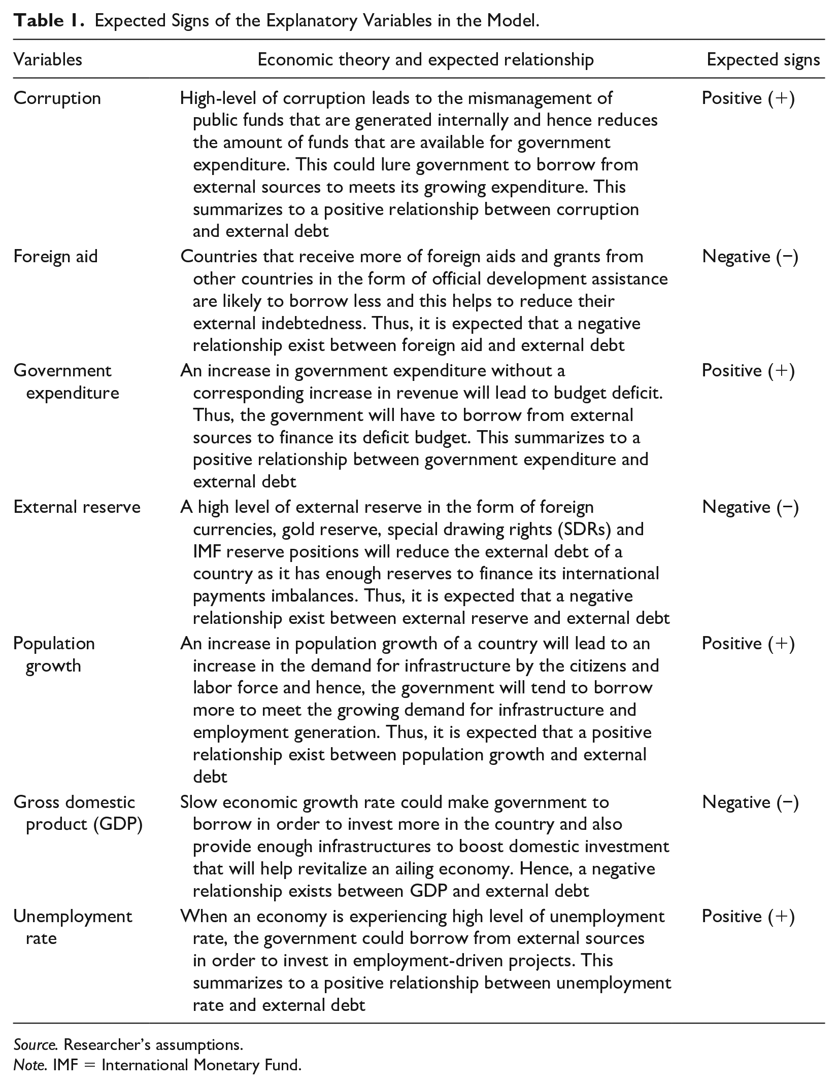
Table 1 shows the expected signs of the explanatory variables in the model.

Table 1.

Expected Signs of the Explanatory Variables in the Model.

Variables	Economic theory and expected relationship	Expected signs
Corruption	High-level of corruption leads to the mismanagement of public funds that are generated internally and hence reduces the amount of funds that are available for government expenditure. This could lure government to borrow from external sources to meets its growing expenditure. This summarizes to a positive relationship between corruption and external debt	Positive (+)
Foreign aid	Countries that receive more of foreign aids and grants from other countries in the form of official development assistance are likely to borrow less and this helps to reduce their external indebtedness. Thus, it is expected that a negative relationship exist between foreign aid and external debt	Negative (−)
Government expenditure	An increase in government expenditure without a corresponding increase in revenue will lead to budget deficit. Thus, the government will have to borrow from external sources to finance its deficit budget. This summarizes to a positive relationship between government expenditure and external debt	Positive (+)
External reserve	A high level of external reserve in the form of foreign currencies, gold reserve, special drawing rights (SDRs) and IMF reserve positions will reduce the external debt of a country as it has enough reserves to finance its international payments imbalances. Thus, it is expected that a negative relationship exist between external reserve and external debt	Negative (−)
Population growth	An increase in population growth of a country will lead to an increase in the demand for infrastructure by the citizens and labor force and hence, the government will tend to borrow more to meet the growing demand for infrastructure and employment generation. Thus, it is expected that a positive relationship exist between population growth and external debt	Positive (+)
Gross domestic product (GDP)	Slow economic growth rate could make government to borrow in order to invest more in the country and also provide enough infrastructures to boost domestic investment that will help revitalize an ailing economy. Hence, a negative relationship exists between GDP and external debt	Negative (−)
Unemployment rate	When an economy is experiencing high level of unemployment rate, the government could borrow from external sources in order to invest in employment-driven projects. This summarizes to a positive relationship between unemployment rate and external debt	Positive (+)

Source. Researcher’s assumptions.

Note. IMF = International Monetary Fund.

Estimation Techniques

To address the stationarity properties of the time-series, panel data unit root tests are performed to determine whether or not the observed country-specific time series for the variables exhibit stochastic trends. We use unit root test proposed by Im et al. (2003), also known as IPS, and Fisher (1932)-type test using Augmented Dickey-Fuller (ADF) and Phillips-Perron (PP) Test. Next, co-integration analysis is performed to examine whether the variables are co-integrated (i.e., whether there are stable long-term equilibrium relationships among them) to avoid spurious regressions.

Both static panel data estimation techniques and panel fully modified ordinary least squares (FMOLS) are employed in the estimation of the empirical models. Static panel data models are usually estimated using either fixed- or random-effect techniques. These two techniques have been developed to handle the systematic tendency of individual-specific components to be higher for some units than for others. The two most widely used techniques for the analysis of a panel data set are the fixed-effects model and the random-effects model. The fixed-effects model assumes that the unobservable country-specific effects are fixed parameters to be estimated along with the coefficients of the model. In the random-effects model (sometimes called the error component model), the unobservable country-specific effect is assumed to be a random disturbance that is distributed independently of the idiosyncratic or “remainder” disturbance that varies over time as well as across countries. A limitation of the random-effects model is that its parameter estimates will be consistent only if the unobserved country-specific component of the disturbance is uncorrelated with the model’s explanatory variables. In the fixed-effects model, on the other hand, the estimators are consistent regardless of whether the country-specific effects are correlated with the regressors. However, the fixed-effects model has at least two limitations of its own. First, since that approach involves estimating the country-specific effect for each country in the panel, the loss of degrees of freedom can be severe. Second, the fixed-effects estimator is incapable of estimating the coefficients of any explanatory variables which vary across countries but are invariant over time, since these are not identified in that model.

In examining the determinants of external indebtedness, we were anxious to explore the effects of time-invariant variables as well as those that vary over time in each country. Therefore, we initially attempted to estimate the model coefficients using the random-effects model. Once those estimates were obtained, however, Hausman’s (1978) specification test was used to test the null hypothesis of no correlation between the regressors and the individual country-specific random effects.

The panel FMOLS is employed in the estimation of the empirical models. FMOLS suggested by Phillips and Hansen (1990) are used. The FMOLS is employed to accommodate considerable heterogeneity across individual members of the panel. It is useful for heterogeneous co-integrated panels. Finally, we proceed with the Panel Granger Causality Test to determine the causal relationship between the variables.

Analysis and Discussion of Results

Panel Unit Root Test and Co-integration Test

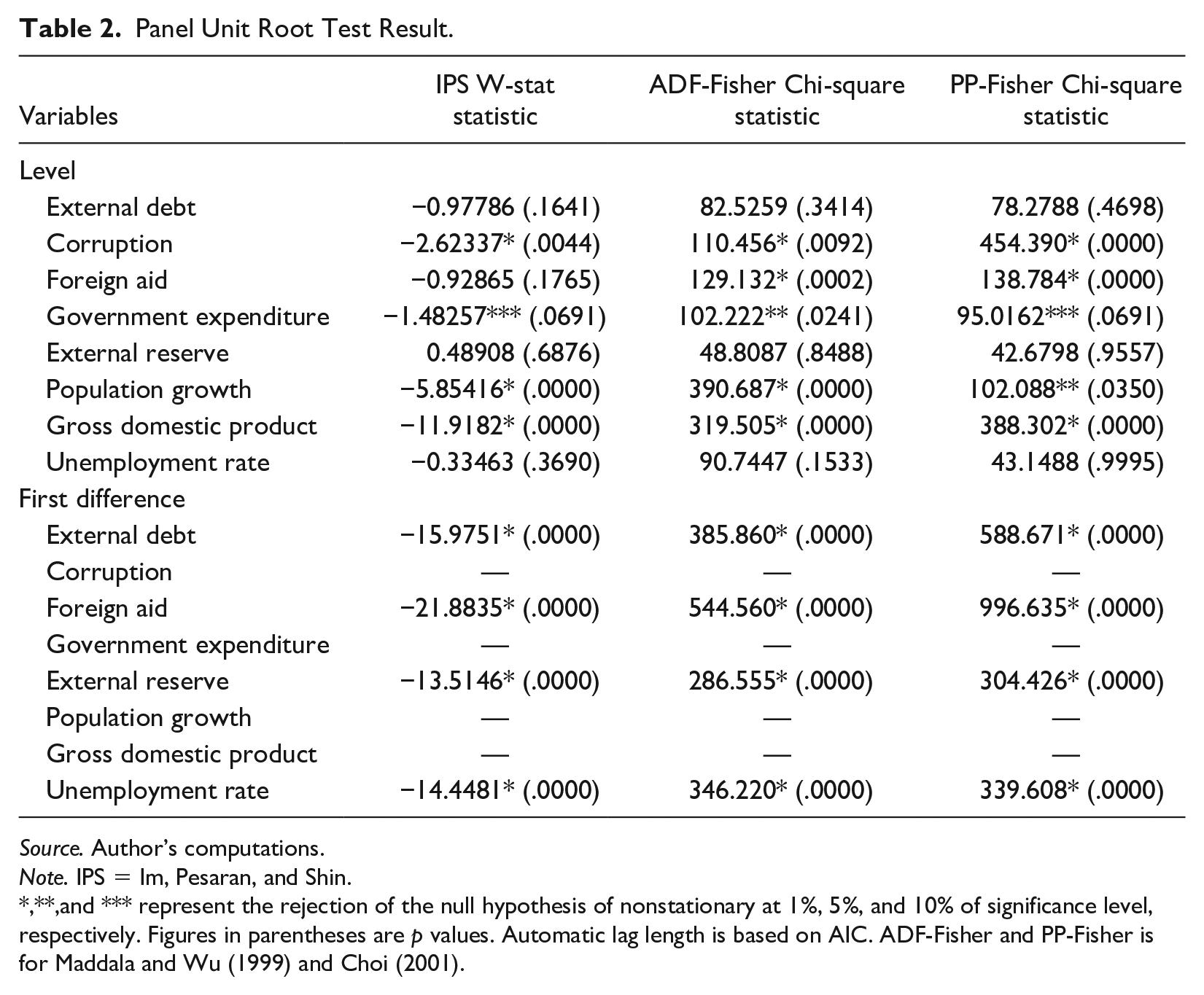
The panel unit root test statistics as shown in Table 2 suggest that only corruption, government expenditure, population growth, and GDP are stationary at level at 1%, 5%, and 10% significance level. External debt, foreign aid, external reserve, and unemployment rate are stationary at first-difference at 1% level of significance. Therefore, we can conclude that the panel variables in our study are integrated of level zero, I(0), and order one, I(1).

Table 2.

Panel Unit Root Test Result.

Variables	IPS W-stat statistic	ADF-Fisher Chi-square statistic	PP-Fisher Chi-square statistic
Level
External debt	−0.97786 (.1641)	82.5259 (.3414)	78.2788 (.4698)
Corruption	−2.62337* (.0044)	110.456* (.0092)	454.390* (.0000)
Foreign aid	−0.92865 (.1765)	129.132* (.0002)	138.784* (.0000)
Government expenditure	−1.48257*** (.0691)	102.222** (.0241)	95.0162*** (.0691)
External reserve	0.48908 (.6876)	48.8087 (.8488)	42.6798 (.9557)
Population growth	−5.85416* (.0000)	390.687* (.0000)	102.088** (.0350)
Gross domestic product	−11.9182* (.0000)	319.505* (.0000)	388.302* (.0000)
Unemployment rate	−0.33463 (.3690)	90.7447 (.1533)	43.1488 (.9995)
First difference
External debt	−15.9751* (.0000)	385.860* (.0000)	588.671* (.0000)
Corruption	—	—	—
Foreign aid	−21.8835* (.0000)	544.560* (.0000)	996.635* (.0000)
Government expenditure	—	—	—
External reserve	−13.5146* (.0000)	286.555* (.0000)	304.426* (.0000)
Population growth	—	—	—
Gross domestic product	—	—	—
Unemployment rate	−14.4481* (.0000)	346.220* (.0000)	339.608* (.0000)

Source. Author’s computations.

Note. IPS = Im, Pesaran, and Shin.

,**,and *** represent the rejection of the null hypothesis of nonstationary at 1%, 5%, and 10% of significance level, respectively. Figures in parentheses are p values. Automatic lag length is based on AIC. ADF-Fisher and PP-Fisher is for Maddala and Wu (1999) and Choi (2001).

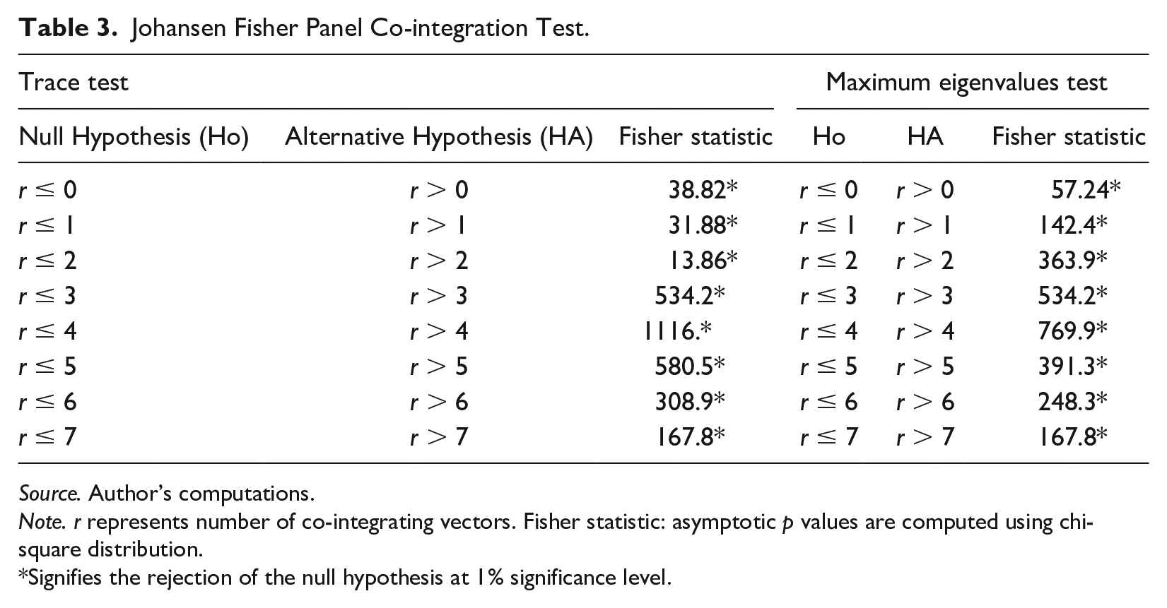
Since not all the variables are integrated of the same order, a co-integration test is performed to determine whether the variables have a long-run relationship. The co-integration test for the external debt model is based on the Johansen Fisher test. Unlike other panel co-integration tests such as Pedroni (1999), the Johansen Fisher test is able to handle a combination of I(0) and I(1) series. The result of the co-integration test in Table 3 shows that all the variables of the model are jointly co-integrated and have a long-run relationship.

Table 3.

Johansen Fisher Panel Co-integration Test.

Trace test			Maximum eigenvalues test
Null Hypothesis (Ho)	Alternative Hypothesis (HA)	Fisher statistic	Ho	HA	Fisher statistic
r ≤ 0	r > 0	38.82*	r ≤ 0	r > 0	57.24*
r ≤ 1	r > 1	31.88*	r ≤ 1	r > 1	142.4*
r ≤ 2	r > 2	13.86*	r ≤ 2	r > 2	363.9*
r ≤ 3	r > 3	534.2*	r ≤ 3	r > 3	534.2*
r ≤ 4	r > 4	1116.*	r ≤ 4	r > 4	769.9*
r ≤ 5	r > 5	580.5*	r ≤ 5	r > 5	391.3*
r ≤ 6	r > 6	308.9*	r ≤ 6	r > 6	248.3*
r ≤ 7	r > 7	167.8*	r ≤ 7	r > 7	167.8*

Source. Author’s computations.

Note. r represents number of co-integrating vectors. Fisher statistic: asymptotic p values are computed using chi-square distribution.

Signifies the rejection of the null hypothesis at 1% significance level.

Panel Data Empirical Results

Table 4.

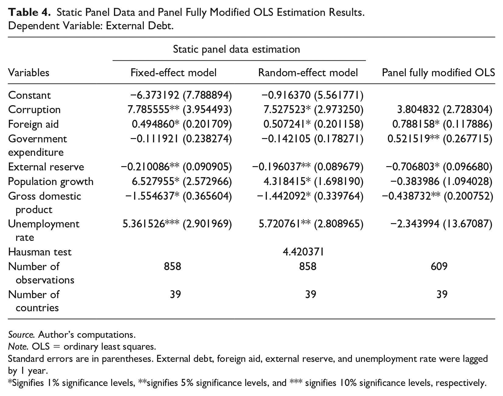
Static Panel Data and Panel Fully Modified OLS Estimation Results.

Dependent Variable: External Debt.

Variables	Static panel data estimation		Panel fully modified OLS
Variables	Fixed-effect model	Random-effect model	Panel fully modified OLS
Constant	−6.373192 (7.788894)	−0.916370 (5.561771)
Corruption	7.785555** (3.954493)	7.527523* (2.973250)	3.804832 (2.728304)
Foreign aid	0.494860* (0.201709)	0.507241* (0.201158)	0.788158* (0.117886)
Government expenditure	−0.111921 (0.238274)	−0.142105 (0.178271)	0.521519** (0.267715)
External reserve	−0.210086** (0.090905)	−0.196037** (0.089679)	−0.706803* (0.096680)
Population growth	6.527955* (2.572966)	4.318415* (1.698190)	−0.383986 (1.094028)
Gross domestic product	−1.554637* (0.365604)	−1.442092* (0.339764)	−0.438732** (0.200752)
Unemployment rate	5.361526*** (2.901969)	5.720761** (2.808965)	−2.343994 (13.67087)
Hausman test	4.420371
Number of observations	858	858	609
Number of countries	39	39	39

Source. Author’s computations.

Note. OLS = ordinary least squares.

Standard errors are in parentheses. External debt, foreign aid, external reserve, and unemployment rate were lagged by 1 year.

Signifies 1% significance levels, **signifies 5% significance levels, and *** signifies 10% significance levels, respectively.

Discussion of Results

In the estimation of the external debt equation, the Hausman specification test (Hausman, 1978) is employed to determine whether fixed or random-effect model is preferable. If the p value of the chi-square statistic is significant, we reject the null hypothesis and accept the alternative hypothesis that fixed-effect model is appropriate. From the analysis, the chi-square statistic (4.420371) of the Hausman test result is insignificant. Therefore, we accept the null hypothesis that random-effect model is appropriate. Consequently, the interpretation of results is based on the random-effect and FMOLS models.

In line with a prior expectation, there is a positive impact of corruption on external debt in HIPCs (Table 4). However, the impact is high across all the models as the coefficient shows a strong positive relationship. In terms of the level of significance, the random-effect model shows a significant relationship between corruption and external debt at 1% level while it is insignificant with the FMOLS. This positive and significant relationship shows that the external indebtedness of the HIPCs is mainly influenced by high level of corruption that leads to the mismanagement of public funds that are generated internally. Thus, if this mismanagement of internally generated funds becomes so high to the extent that they are no longer enough to meet the needs of the citizens, the government resorts to borrowing from external sources to complement the dearth in revenue. This supports the arguments of Tiruneh (2004) that irresponsible and corrupt governments (sometimes unelected ones) in developing countries themselves are the key players of the debt build-up. He cited the case of Mobutu of Zaire, who shamelessly squandered their nations’ scarce resources for luxurious activities rather than investing them to improve the lives of the desperately poor nations. Most political office holders in these countries who receive contracts to execute capital projects tend to divert it for their own personal gains by acquiring luxuries rather than utilizing it for the purpose for which they are meant for. The positive relationship is consistent with the findings of Cooray and Schneider (2013) and Luigi et al. (2015) who found out that corruption leads to an increase in public debt.

The estimated impact of foreign aid on external debt is positive and statistically significant in all the models. This is contrary to the a priori expectation that countries that receive more of foreign aids and grants from other countries in the form of ODA are likely to borrow less and this helps to reduce their external indebtedness. This shows that the external indebtedness of HIPCs is as a result of an increase in foreign aid. This could be attributed to the fact that when a country receives more of foreign aids from a country, they may become dependent on such country and may be inclined to borrow more from them in times of needs and emergency situations. The result is consistent with the findings of Bader and Magableh (2009).

The impact of government expenditure on external debt is mixed and unstable; while it is negative in the random-effect model, it is positive in the FMOLS model. However, the positive effect is stronger and more significant than that of the negative effect. The significant positive effect indicates that increase in government expenditure stimulates external indebtedness in HIPCs. This is so because in these countries, the government spends more than the revenue it generates and the end result is a deficit budget. Hence, the government is inclined to borrow more to finance its deficit budget. The result of Murwirapachena and Kapingura (2015) revealed that external debt in South Africa is mainly driven by high levels of government spending on infrastructure.

External reserve has a significant negative impact on external debt, indicating that external reserve could be beneficial, especially for financing international payments imbalances and hence limiting the government from accumulating huge amount of external debt. This disagrees with the findings of Alfaro and Kanczuk (2009). The relationship between population growth and external debt is also mixed. It exhibits a positive relationship in the random-effect model but negative in the FMOLS model. However, the positive effect is stronger and more significant than that of the negative effect. This positive and significant relationship is evidence from the fact that the population of the HIPCs increases much faster than their available resources and hence, the government in the quest to cater for the teaming population in terms of providing more infrastructure and employment opportunities resort to foreign borrowing.

Furthermore, GDP has a negative and significant impact on external debt in the entire model, which is as expected and consistent with economic theory that higher economic growth should certainly diminish the pressure on internal and external borrowing (Globan & Matosec, 2016). Pyeman et al. (2014) and Bittencourt (2015) support the argument that higher economic growth reduces the external indebtedness of a country.

Finally, unemployment rate has a positive and significant relationship with external debt in the random-effect model and hence authenticating the economic theory that when an economy is experiencing high level of unemployment rate, the government could borrow from external sources in order to invest in employment-driven projects. HIPCs are mostly faced with high rate of unemployment which makes government to accumulate more debt that will be invested in capital projects that will likely create more jobs.

Panel Granger Causality Test

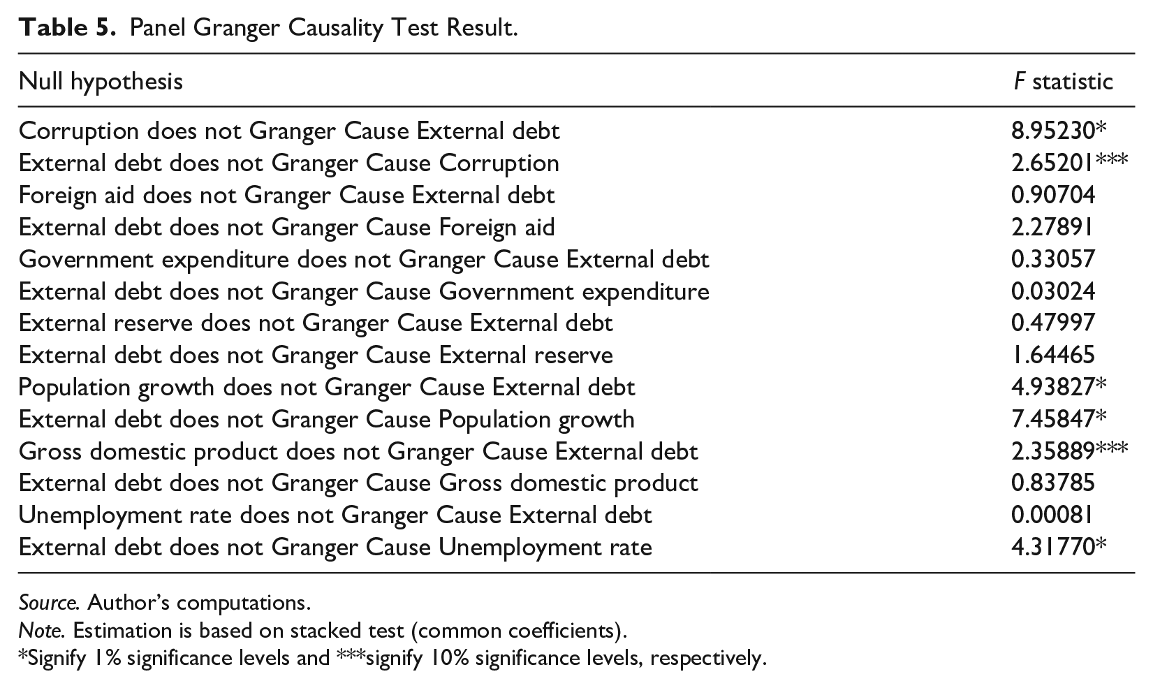
Finally, we proceed to test whether there is any causal relationship between corruption, foreign aid, government expenditure, external reserve, population growth, GDP and unemployment rate, and external debt in HIPCs as captured in the model. According to Engle and Granger (1987), if two variables are co-integrated, then there is possibility of causality between the two at least in one direction. The result of the Panel Granger Causality Test is presented in Table 5.

Table 5.

Panel Granger Causality Test Result.

Null hypothesis	F statistic
Corruption does not Granger Cause External debt	8.95230*
External debt does not Granger Cause Corruption	2.65201***
Foreign aid does not Granger Cause External debt	0.90704
External debt does not Granger Cause Foreign aid	2.27891
Government expenditure does not Granger Cause External debt	0.33057
External debt does not Granger Cause Government expenditure	0.03024
External reserve does not Granger Cause External debt	0.47997
External debt does not Granger Cause External reserve	1.64465
Population growth does not Granger Cause External debt	4.93827*
External debt does not Granger Cause Population growth	7.45847*
Gross domestic product does not Granger Cause External debt	2.35889***
External debt does not Granger Cause Gross domestic product	0.83785
Unemployment rate does not Granger Cause External debt	0.00081
External debt does not Granger Cause Unemployment rate	4.31770*

Source. Author’s computations.

Note. Estimation is based on stacked test (common coefficients).

Signify 1% significance levels and ***signify 10% significance levels, respectively.

The results of the Granger Causality Test as presented in Table 5 shows that there is a bi-directional causal relationship between corruption and external debt with a feedback effect from external debt to corruption as the probability value of the F-statistics in significant at 1% and 10% level respectively. This shows that corruption triggers external debt of HIPCs within the period under study. This helps to authenticate our earlier findings of a positive and significant impact of corruption on external debt. This point to the fact that corruption is indeed inimical to an economy as it leads to the mismanagement of scarce resources and higher debt accumulation.

However, there is no causal relationship between foreign aid and external debt, government expenditure and external debt and external reserve and external debt in both directions as the F-statistics is insignificant. But nonetheless, population growth has a bi-directional causal relationship with external debt. Population growth triggers external debt as when the resources of a country is no longer enough to meet the needs of the people, borrowing becomes an option for the government. This also corroborates our earlier findings which show a positive and significant relationship between population growth and external debt.

Finally, there is a unidirectional causality between GDP and external debt as GDP triggers external debt at 10% significant level but on the contrary, external debt does not triggers GDP. This causal relationship between GDP is provides a strong support for our earlier findings that GDP has a negative and significant relationship with external debt. This is evidence from the fact that a growing economy is likely to borrow less than a recessed economy as one of the major reasons why countries borrow is to invest in capital projects and infrastructures that will likely spur economic growth. That of unemployment rate shows a unidirectional causality, as it is external debt that triggers unemployment rate and not the other way round. This is so because a country that has accumulated huge level of external debt will concentrate mainly on servicing the debt and may allocate more resources in servicing the debt and this may likely retard investment in projects that are likely to create more jobs.

Concluding Remarks and Recommendations

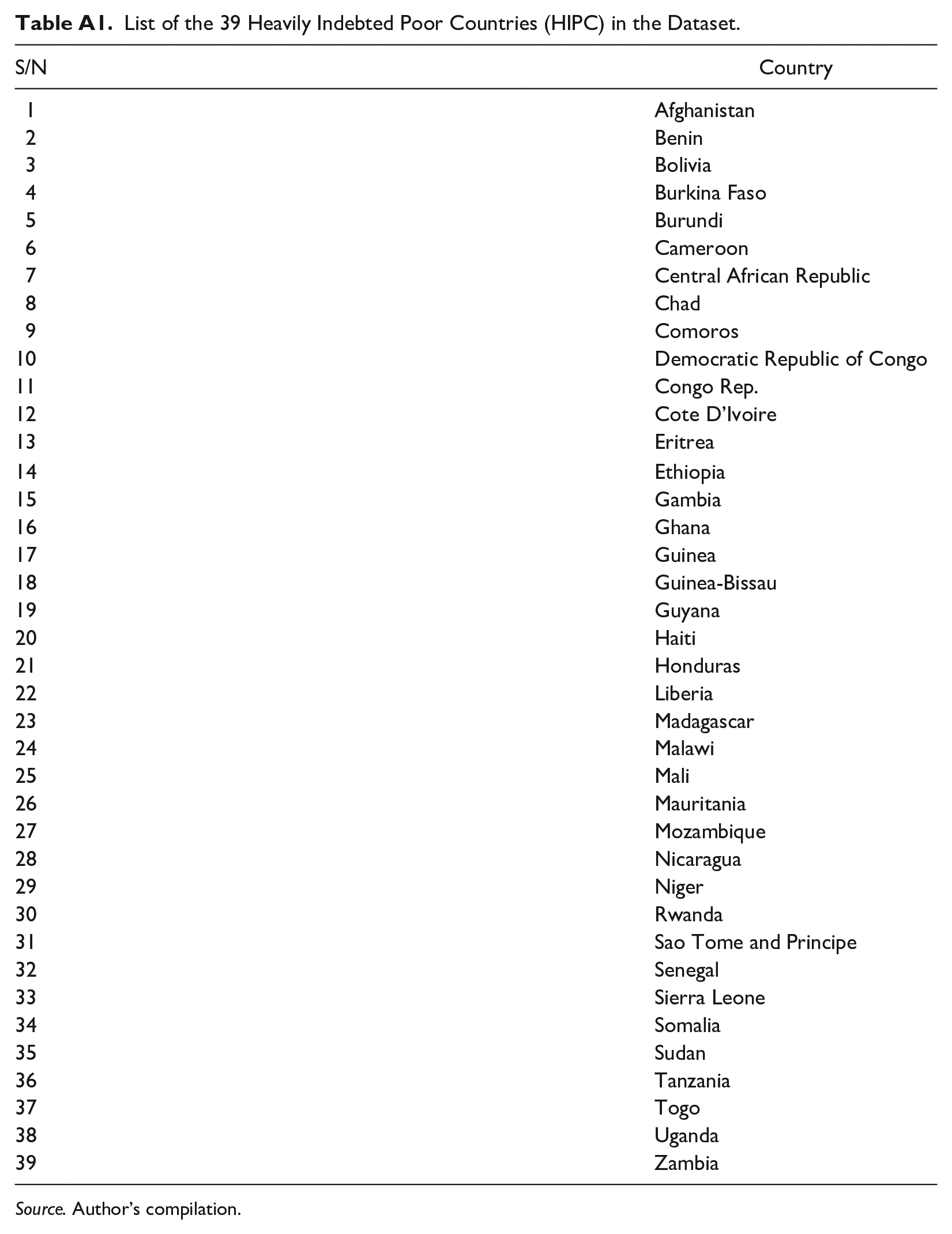
This study specifically examined the determinants of external indebtedness using macroeconomic and socio-economic factors such as corruption, foreign aid, government expenditure, external reserve, population growth, economic growth, and unemployment rate by employing a panel data set of all the 39 HIPCs covering period of 1996 when the HIPC initiatives was introduced by the IMF and World Bank to the end period of 2018 (Appendix Table A1). Both static panel data estimation and panel fully modified OLS were employed in the study in estimating the relevant relationship between the variables.

The result of the analysis has proven that corruption matters in increasing the external indebtedness of HIPCs while foreign aid does not matter in reducing their external indebtedness as it resulted to higher external debt accumulation. An increase in external debt is positively and significantly associated with high rate of corruption and dependency on foreign aids. This positive and significant relationship between corruption and external debt corroborated our Granger Causality Test result which shows that corruption triggers external debt and as such, the government of HIPCs should fight corruption to the barest minimum so as to reduce the level of external debt accumulation. A major way to achieve this is to institute a monitoring team to be constituted by both indigenous and foreign personnel and such foreign personnel should not come from a sister country, which will oversee funds that are disbursed to political office holders. Indigenous personnel should not be allowed to make up a monitoring team for public funds as the foreign personnel will act as a watchdog to ensure transparency and proper accountability in the utilization of public funds that are meant for economic projects. This measure will ensure effective and efficient utilization of internally generated funds and will invariably reduce the level of government borrowings. Also, the Government should impose strict measures that will ensure that funds meant for projects are sent directly to contractor’s bank account rather than disbursing it to unscrupulous political office holders that will end up diverting it for their own private gains. This will ensure that public funds are utilized for the purpose for which they are meant for.

Also, we found out that Government expenditure has an increasing effect on external indebtedness of HIPCs and as such, the government should limit it spending based on the amount of revenue it generate to avoid the issue of budget deficit of which the end result is external borrowing. External reserve on the other hand, has a reducing effect on external debt, and hence, the government should pursue and effective and efficient external reserve management.

In addition, the high population growth rate of the HIPCs seems to correlate positively with external debt while GDP exhibited a negative relationship and the findings are robust to a Granger causality and as such the government should pursue a stable population growth rate and a sustained economic growth. In line with the theoretical expectation, unemployment rate strongly impacts negatively on external debt and thus, the Government should promote entrepreneurship and skill acquisition training program so as to encourage people to be job creators rather than job seekers. This will help reduce the pressure on the government for jobs. This will reduce the rate of unemployment and will avoid luring government to borrow in order to create more jobs.

Footnotes

Appendix

Table A1.

List of the 39 Heavily Indebted Poor Countries (HIPC) in the Dataset.

S/N	Country
1	Afghanistan
2	Benin
3	Bolivia
4	Burkina Faso
5	Burundi
6	Cameroon
7	Central African Republic
8	Chad
9	Comoros
10	Democratic Republic of Congo
11	Congo Rep.
12	Cote D’Ivoire
13	Eritrea
14	Ethiopia
15	Gambia
16	Ghana
17	Guinea
18	Guinea-Bissau
19	Guyana
20	Haiti
21	Honduras
22	Liberia
23	Madagascar
24	Malawi
25	Mali
26	Mauritania
27	Mozambique
28	Nicaragua
29	Niger
30	Rwanda
31	Sao Tome and Principe
32	Senegal
33	Sierra Leone
34	Somalia
35	Sudan
36	Tanzania
37	Togo
38	Uganda
39	Zambia

Source. Author’s compilation.

Declaration of Conflicting Interests

The author(s) declared no potential conflicts of interest with respect to the research, authorship, and/or publication of this article.

Funding

The author(s) received no financial support for the research, authorship, and/or publication of this article.

ORCID iD

Chukwuebuka Bernard Azolibe

Author Biography

Chukwuebuka Bernard Azolibe is working on a Master’s in Banking at the Nnamdi Azikiwe University Awka, Nigeria. His research interests include development economics, applied economics, financial intermediation, and public finance. His current work involves infrastructure development and industrial sector productivity in Sub-Saharan Africa.

References

Abdullahi

M. M.

Bakar

N. A. B. A.

Hassan

S. B.

(2015). Determining the macroeconomic factors of external debt accumulation in Nigeria: An ARDL bound test approach. Procedia—Social and Behavioral Sciences, 211, 745–752.

Alberto

Beatrice

(1999). Do corrupt government receive less foreign aid? (NBER Working Paper No. 7108). National Bureau of Economic Research.

Alfaro

Kanczuk

(2009). Optimal reserve management and sovereign debt. Journal of International Economics, 77(1), 23–36.

Arusha

Friedrich

G. S.

(2013). How does corruption affect public debt? An empirical analysis (MPRA Working Paper No. 1322). Johannes Kepler University of Linz.

Awan

Asghar

Rehman

H. U.

(2011). The impact of exchange rate, fiscal deficit and terms of trade on external debt of Pakistan. Australian Journal of Business and Management Research, 1(3), 10–24.

Bader

Magableh

I. K.

(2009). An enquiry into the main determinants of public debt in Jordan: An econometric study. Dirasat: Administrative Sciences, 36(1), 181–190.

Barungi

B. M.

Atingi

(1997). Growth and foreign debt: The Ugandan experience (AERC Research Paper No. 66). African Economic Research Consortium.

Belguith

S. O.

Omrane

(2017). Macroeconomic determinants of public debt growth: A case study for Tunisia. Theoretical and Applied Economics, 24(4), 161–168.

Bittencourt

. (2015). Determinants of government and external debt: Evidence from the young democracies of South America. Emerging Markets Finance and Trade, 51(3), 463–472.

10.

Bjerg

Bjørnskov

Holm

(2007). Growth, debt burdens and alleviating effects of foreign aid in least developed countries (Working Paper No. 07-1, 1-23). Aarhus School of Business.

11.

Brafu-Insaidoo

W. G.

Ahiakpor

Ogeh

F. V.

Cantah

W. G.

(2019). Macro-determinants of short-term foreign debt in Ghana. Cogent Economics & Finance, 7(1), 1–17.

12.

Bullow

Rogoff

(1989). Sovereign debt: Is to forgive and forget? The American Economic Review, 79(1), 43–50.

13.

Choi

(2001). Unit root tests for panel data. Journal of International Money and Finance, 20(2), 249–272.

14.

Cooray

Schneider

(2013). How does corruption affect public debt? An empirical analysis (Working Paper No. 1322). Johannes Kepler University of Linz.

15.

Craig

Courtney

Roger

. (2006). Corruption and credit worthiness. Evidence from sovereign credit ratings (Working Paper No. 1). University of Texas.

16.

Easterly

(2002). How did heavily indebted poor countries become heavily indebted? Reviewing two decades of debt relief. World Development, 30(10), 1677–1696.

17.

Eaton

Gersovitz

(1981). Debt with potential repudiation: Theoretical and empirical analysis. The Review of Economic Studies, 48(2), 289–309.

18.

Engle

R. F.

Granger

C. W.

(1987). Cointegration and error correction: Representation, estimation and testing. Econometrica, 55(2), 251–276.

19.

Ferraro

Rosser

(1994). Global debt and third world development. In Klare

Thomas

(Eds.), World security: Challenges for a new country (pp. 332–335). St. Martin’s Press.

20.

Fisher

R. A.

(1932). Statistical methods for research workers (4th ed.). Oliver & Boyd.

21.

Globan

Matosec

(2016). Public debt-to-GDP ratio in new EU member states: Cut the numerator or increase the denominator? Romanian Journal of Economic Forecasting, 19(3), 57–72.

22.

Greenidge

Drakes

Craigwell

(2010). The external public debt in the Caribbean community. Journal of Policy Modelling, 32(1), 418–431.

23.

Hajivassiliou

V. A.

(1987). The external debt repayments problems of LDC’s: An econometric model based on panel data. Journal of Econometrics, 36(1), 205–230.

24.

Hausman

J. A.

(1978). Specification tests in econometrics. Econometrica, 46(6), 1251–1271.

25.

K. S.

Pesaran

M. H.

Shin

(2003). Testing for unit roots in heterogeneous panels. Journal of Econometrics, 115(1), 53–74.

26.

International Monetary Fund. (2000, April 5). Press release: IMF and IDA support debt relief for Tanzania. https://www.imf.org/en/News/Articles/2015/09/14/01/49/pr0026

27.

International Monetary Fund. (2017). Debt relief under the heavily indebted poor countries (HIPC) initiative (IMF Factsheet).

28.

Kaufmann

Kraay

Mastruzzi

(2006). Measuring corruption: Myths and realities. http://www1.worldbank.org/publicsector/anticorrupt/corecourse2007/Myths.pdf

29.

Lau

Lee

A. S.

(2016). Determinants of external debt in Thailand and the Philippines. International Journal of Economics and Financial Issues, 6(4), 1973–1980.

30.

Luigi

Alfredo

D. M.

Lucca

(2015). Corruption and public debt: An empirical analysis (Working Paper No. 1). University of Naples, Federico II and CSEF.

31.

Maddala

G. S.

(1999). A comparative study of unit root tests with panel data and a new simple test. Oxford Bulletin of Economics and Statistics, 61(S1), 631–652.

32.

Malito

D. V.

(2014). Measuring corruption indicators and indices (RSCAS Research Paper No. 2014/13). European University Institute.

33.

Murwirapachena

Kapingura

F. M.

(2015). Determinants of external debt in South Africa: A VAR-based approach. International Journal of Economic Policy in Emerging Economies, 8(2), 138–152.

34.

Özata

(2017). Determinants of external debt accumulation in Turkey: Evidence from an ARDL bound test approach. Journal of Business & Economic Policy, 4(4), 134–143.

35.

Pedroni

(1999). Critical values for cointegration tests in heterogeneous panels with multiple regressors. Oxford Bulletin of Economics and Statistics, 61(S1), 653–670.

36.

Phillips

P. C. B.

Hansen

B. E.

(1990). Statistical inference in instrumental variables regression with I(I) processes. Review of Economics Studies, 57(1), 99–125.

37.

Pyeman

Noor

Mohamad

Yahya

(2014). Factors affecting external debt in Malaysia: An empirical investigation. In Proceedings of the first AAGBS International Conference on Business Management. Springer.

38.

Qerimi

Sergi

B. S.

(2012a). The boundaries of a neglected relationship: Corruption and economic freedom. Problems of Economic Transition, 55(2), 68–97.

39.

Qerimi

Sergi

B. S.

(2012b). The effects of economic freedom on institutional performance in the Western Balkans countries. International Journal of Business Governance and Ethics, 7(1), 18–36.

40.

Rahman

(2012). How federal government’s debt affect the level of economic growth? International Journal of Trade, Economics and Finance, 3(4), 323–326.

41.

Roodman

(2001). Still waiting for the jubilee: Pragmatic solutions for the third world debt crisis (Worldwatch Paper No. 155). Worldwatch Institute.

42.

Sinha

Arora

Bansal

(2011). Determinants of public debt for middle income and high income group countries using panel data regression (MPRA Paper No. 32079). University of Delhi.

43.

Swamy

(2015). Government debt and its macroeconomic determinants. An empirical investigation (MPRA Paper No. 64106). https://mpra.ub.uni-muenchen.de/64106/

44.

Tiruneh

M. W.

(2004). An empirical investigation into the determinants of external indebtedness. Prague Economic Papers, 3, 261–277.

45.

Walsh

(2019, April 20). Mozambique cyclone wiped out the nation’s food. Now aid is in short supply. The New York Times. https://www.nytimes.com/2019/04/20/world/africa/mozambique-cyclone.html

46.

World Bank. (2018). World development indicators.

47.

World Bank. (2019). Worldwide governance indicators. https://info.worldbank.org/governance/wgi/