Sociospatial Dimensions of Water Injustice: The Distribution of Surface Water Toxic Releases in California’s Bay-Delta

Abstract

Previous water injustice research focuses predominantly on inequities and power relations in water use, management, governance, and rights. This article charts a new research direction with a case study of the unequal distribution of surface water toxic release hazard levels across census block groups in California’s Bay-Delta region in the year 2000. The article draws on secondary data and geographic information systems, as well as spatial regression analyses to test intersectional environmental inequality hypotheses regarding the determinants of surface water cumulative areal-weighted modeled hazard scores (CAWMHS)—a new environmental health hazard indicator derived in this study from the U.S. Environmental Protection Agency Risk-Screening Environmental Indicators database. Spatial error regression models demonstrate that black disadvantage and isolated Latino disadvantage are the strongest and positive demographic determinants of surface water CAWMHS, net of other factors. Findings have scholarly and practical implications for environmental inequality and water injustice research and policy.

Keywords

environmental inequality water injustice intersectionality spatial analysis U.S. EPA Risk-Screening Environmental Indicators

Introduction

A vast social science literature on environmental inequality and justice has developed over the last 40 years to illuminate the social and spatial factors contributing to the unequal distribution of environmental benefits and burdens in the United States and abroad. The environmental justice concerns in the U.S. context have historically included the production, distribution, and disposal of hazardous waste and other toxic substances; land use; and equitable access to affordable housing, transportation, and water (Brown 2007). More recently, environmental justice concerns include climate vulnerabilities and unequal food access (Mohai, Pellow, and Roberts 2009).

The present study focuses on the problem of “water injustice,” which has garnered increasing attention from scholars, advocates, and regulators in recent years. Water injustice typically refers to the unequal distribution of rights to access healthy and affordable water, the lack of meaningful participation in water governance, and the misrecognition of culturally diverse ways of equitably and sustainably managing the interaction between water systems and social systems (Zwarteveen and Boelens 2014). The importance of water injustice cannot be understated as “20% of the world’s 7 billion people lack easy access to water for basic subsistence needs and a variety of economic and household activities” (Lu, Ocampo-Raeder, and Crow 2014:129), while “80% of wastewater is not collected and treated, with [potentially unequal] negative consequences for health, ecological service provision and socio-economic development” (Swyngedouw 2014:258). Recent scholarly attention to water injustice has culminated in international, cross-disciplinary workshops on the multi-scalar dimensions of equitable water governance (see Lu et al. 2014). However, those efforts have neglected the sociospatial dimensions of water injustice that relate to broader environmental inequality research on the relationship between community context, proximity to toxic releases, and the relative health hazards of such releases (Chakraborty, Maantay, and Brender 2011). At stake in such omission is a fuller understanding of the distributional aspects of water injustice and the extent to which such patterns reflect environmental inequalities witnessed in earlier research on air- and land-based toxic releases.

I use a case study of the unequal distribution of surface water toxic releases in California’s San Francisco Bay–Sacramento-San Joaquin Delta (Bay-Delta) region to chart a new direction in research on the sociospatial dimensions of water injustice. California’s Bay-Delta provides a useful context for such object of inquiry. It has relatively high degree of water pollution, socially unequal risk of exposure to such pollution through subsistence fish consumption, and a history of inequitable water governance (F. M. Shilling, London, and Liévanos 2009; F. Shilling et al. 2010; Silver et al. 2007; Sze et al. 2009). These and other factors suggest it may have external validity to comparable U.S. watersheds such as the Chesapeake Bay, the Columbia River Basin, the Florida Everglades, and the Mississippi River Delta (Heikkila and Gerlak 2005).

This case study draws on secondary data, geographic information systems, and spatial regression analysis to test intersectional environmental inequality hypotheses regarding the determinants of surface water cumulative areal-weighted modeled hazard scores (CAWMHS) at the census block group level for the year 2000. The analysis contributes to previous literature on water injustice and the sociospatial dimensions of environmental inequality outcomes in two important ways. First, this article develops the novel CAWMHS measure, which represents the plausible block group-level cumulative health hazard of proximate surface water toxic releases for the year 2000 in the California Bay-Delta region. It was created by adapting and synthesizing techniques of previous air- and land-based environmental inequality outcomes research using distanced-based environmental hazard proximity measures (Mohai and Saha 2007), health-related modeled hazard scores for toxic releases from the U.S. Environmental Protection Agency (EPA) Risk-Screening Environmental Indicators database (Sicotte and Swanson 2007), and cumulative environmental hazard density indices (Bolin et al. 2002). Second, the article extends recent intersectional environmental inequality outcomes research (e.g., Collins et al. 2011; Liévanos 2015) by illustrating how environmental inequality outcomes in the context of surface water health hazards are dissimilar for socioeconomically disadvantaged whites, blacks, Asian/Pacific Islanders (API), and Latinos, and API- and Spanish-speaking linguistically isolated residential settlements. Spatial regression analyses identify dissimilar water injustice outcomes by race, socioeconomic status, and linguistic ability, and demonstrate that black disadvantage and isolated Latino disadvantage are the strongest positive demographic determinants of surface water CAWMHS net of controls.

The article proceeds as follows. First, I review previous research on water injustice in the California Bay-Delta and additional scholarship on the sociospatial dimensions of environmental inequality in the United States. In so doing, I introduce my case study region and derive intersectional environmental inequality hypotheses that guide my analysis of the sociospatial dimensions of water injustice in that region. I follow with a summary of my data, method, and results. I conclude with a discussion of this article’s scholarly contributions to the study of water injustice and environmental inequality outcomes and its practical implications for addressing the sociospatial dimensions of water injustice in California’s Bay-Delta region.

Literature Review

Water Injustice in California’s Bay-Delta Region

Water justice advocates working in the California Bay-Delta (see Figure 1) demand for “the ability of low-income communities and communities of color to access safe, affordable, clean water for all its many beneficial uses, including drinking, subsistence, recreation and cultural practices” (Vanderwarker 2006:26). They link their water justice advocacy to the patterns of water injustices they claim permeate the region and the rest of California. The following passage from the California-based Environmental Justice Coalition for Water (EJCW) outlines the unequal statewide landscape:

Figure 1.

Six-county California Bay-Delta study area.

Millions of people—largely from low income communities and communities of color—rely on contaminated sources of drinking water and experience a wide range of health problems as a result. California’s low-income communities and communities of color experience watershed-level injustices ranging from the destruction of salmon runs to loss of access to ceremonial springs to mercury contamination of fish to overflows of raw sewage that pollute beaches and swimming places. (EJCW 2005:71)

Previous scholarship supports some advocates’ claims regarding water injustices in the region. For example, case studies of environmental justice-related water management programs tied to the region during the 2000s demonstrated how the region’s low-income, black, Asian, Latino, and Native American populations participating in those initiatives—including representatives from EJCW—were systematically subordinated in those processes (F. M. Shilling et al. 2009; Sze et al. 2009). Joanna L. Robinson (2013) also illustrates how water justice concerns were central to spurring social movement and local community groups’ legal challenge to a 2003 corporate municipal water privatization initiative in the Bay-Delta city of Stockton until it was overturned in 2008.

Other research has focused on the problem of unequal risk of consuming fish contaminated with mercury and other toxins. Such research is noteworthy because it focuses on a key pathway of exposure to industrial surface water toxins (U.S. Environmental Protection Agency [U.S. EPA] 2010b) in a region comprised of numerous popular fishing sites, especially the impaired San Francisco Bay (EJCW 2005:59). Indeed, there is a relatively high degree of local interaction with the region’s surface waters with at least 191,000 of California’s 1.2 million licensed fish anglers (15.92 percent) as of 2001 residing in the region’s Contra Costa, Sacramento, San Joaquin, Solano, and Yolo counties (F. Shilling et al. 2010:337). Fraser Shilling et al. (2010) conducted a survey of anglers and community members in waterways between Bay-Delta cities of Fairfield, Sacramento, and Stockton (see Figure 4). The study found that African Americans, Lao, Vietnamese, other Asian and Pacific Islanders, and Latinos were more likely to have contaminated fish consumption rates that exceeded regulatory health guidelines. Elana Silver et al. (2007) explored the racial-ethnic disparities in fish consumption rates and fish advisory awareness among low-income women at a Stockton welfare health clinic. Figure 1 maps the fish consumption advisories present throughout the region according to data from the U.S. EPA (2015) and the California State Water Resources Control Board (SWRCB; 2008a, 2008b). Figure 2 provides an example of the multilingual fish advisory signs posted throughout the region. Silver et al.’s (2007) study suggests low-income women with low fish advisory awareness and who self-identify as African American and Asian—especially Vietnamese and Cambodian—face the highest contaminated fish consumption risk in Stockton.

Figure 2.

Fish advisory sign in Stockton, California.

Disparate case studies of select Bay-Delta cities suggest unequal residential proximity to water-polluting industrial activity may be evident throughout the region and embedded in patterns of racial segregation and uneven development. Water justice advocates working in the Bay-Delta community of Richmond, for example, argue legacies of race and class inequalities manifest in local real estate markets, land use planning, and water policy have created a contemporary context in that community whereby nonwhite, low-income, and non-English-speaking populations have had their waterways disproportionately polluted from industrial sources, particularly the Richmond Chevron Refinery (Vanderwarker 2006). Historical case studies of Sacramento (Hernandez 2009), Stockton (Liévanos 2013), and Oakland (McClintock 2011) suggest any contemporary relationship between racially segregated residential settlements and proximate industrial pollution in those cities is rooted in the use and enforcement of racially restrictive covenants, central city urban renewal initiatives, mortgage redlining, and intensive industrial development on waterfronts near low-income, non-English-speaking, and nonwhite—especially black or African American—populations.

Previous research demonstrates institutional and population-level dynamics of water injustice are evident in California’s Bay-Delta. However, research has not systematically explored the extent to which residential racial composition, socioeconomic status, and linguistic ability is correlated with proximity to water-polluting industrial activity and the hazardousness of such activity throughout the region. The broader environmental inequality literature contains additional insights that may inform the study of the sociospatial dimensions of water injustice in the Bay-Delta.

Sociospatial Dimensions of Environmental Inequality

The “race-versus-class” debate within sociology has disputed the extent to which the life chances of racialized groups in the contemporary postindustrial period is driven more by legacies of racial discrimination and segregation (Massey and Denton 1993) or political-economic transformations and within-racial group class differences (Wilson 1987, 1996). Despite a few null findings (Mohai et al. 2009; Ringquist 2005), the majority of U.S.-based quantitative environmental inequality research on land- and air-based environmental hazards reflects the broader race-versus-class debate in that it finds varying levels of support for the relative salience of neighborhood-, household-, and individual-level racial or socioeconomic factors in predicting environmental inequality outcomes (Chakraborty et al. 2011; Crowder and Downey 2010; Mohai et al. 2009; Mohai and Saha 2007, 2015; Pastor, Morello-Frosch, and Sadd 2005; Pastor, Sadd, and Morello-Frosch 2004; Sicotte and Swanson 2007; Smith 2007). Attending to the relationship between race, socioeconomic status, and environmental inequality outcomes is important but neglects how those factors and “other social categories are always linked in the experiences of individuals and groups” (Mohai et al. 2009:416). Laura Pulido (1996, 2000) and more recently Liam Downey and Brian Hawkins (2008), Timothy W. Collins et al. (2011), and Raoul S. Liévanos (2015) elaborate on this intersectional notion of environmental inequality by arguing that strictly attending to whether racial or socioeconomic conditions drive environmental inequality outcomes ignores how these factors often combine to produce environmental inequality in complex and uneven ways across different racialized populations.

Downey and Hawkins’s (2008) nationwide, tract-level analysis of cumulative exposure to air-toxic releases from manufacturing facilities in 2000 focuses on the intersections of race, socioeconomic status, and environmental inequality in the United States. They found (1) dissimilar associations between tract-level air-toxic concentrations and black, white, and Latino households; (2) tract and household racial composition mediates the association between tract and household income levels and air-toxic concentrations; and (3) air-toxic concentrations are disproportionately associated with low-income black areas. Relating Downey and Hawkins’s (2008) latter finding to urban sociological research on the “truly disadvantaged” postindustrial, black, “outcast ghetto” in the United States (Marcuse 1997; Wacquant 2008; cf. Wilson 1987) suggests such spaces represent the convergence of race and class stigmatization and subordination, sociopolitical isolation, exclusion from circuits of capital accumulation, and elevated risk of exposure to toxic contamination in contrast to other comparably socially and economically disadvantaged racial groups.

Additional research suggests linguistic abilities can combine with race and socioeconomic factors to produce environmental inequality outcomes in the United States. Collins et al. (2011) found that block group-level Latino poverty rates, percentages of Latinos without a high school diploma, and percentages of Spanish-speaking households with limited English-language proficiency were disproportionately associated with 2002 air-toxic lifetime cancer risk levels in El Paso County, Texas. Similarly, Liévanos’s (2015) factor variable representing economically deprived Latino immigrants and Spanish-speaking, linguistically isolated households was the predominant demographic predictor—among comparable intersectional measures of race, economic deprivation, and immigrant status—of census tract presence in 2005 air-toxic lifetime cancer risk clusters in the continental United States.

Similar intersectional environmental inequality outcomes have been found for Latinos and other racialized groups in California. Luke W. Cole and Sheila R. Foster (2001) document in detail how white elites neglected to translate environmental impact reports into Spanish and thus violated environmental law as they attempted to site a hazardous waste incinerator in the predominantly Latino, Spanish-speaking, and farmworker community of Kettleman City, California. Bindi Shah’s (2008) examination of community response to the 1999 air-toxic flares from the Richmond Chevron Refinery suggests patterns of air-based environmental inequality in the Bay-Delta region that involve the intersection of race, socioeconomic status, and linguistic abilities. As Shah (2008) observes, warning systems to “shelter-in-place” from the toxic flares were either disseminated late or in English-only language formats, which placed the disproportionately low-income, black, Latino, Asian and Pacific Islander (API), and non-English-speaking neighborhoods proximate to the toxic flares at heightened risk of exposure to the toxins.

Hypotheses

Research illustrates how race intersects with socioeconomic status and linguistic ability to provide the basis for exclusive water governance structures and unequal risk of exposure to surface water hazards through subsistence fish consumption in California’s Bay-Delta. However, it is unclear the extent to which such factors at the aggregate level are associated with the unequal social and spatial distribution of health hazards of water-polluting industrial activity throughout the region. Therefore, I propose and test the following three hypotheses, which adapt previous intersectional analyses of the aggregate-level demographic predictors of air-toxic levels (Collins et al. 2011; Downey and Hawkins 2008; Liévanos 2015) for the present study’s focus on the intersections of race, socioeconomic status, linguistic ability, and modeled surface water hazard levels at the block group level in California’s Bay-Delta.

Hypothesis 1: The dissimilar water injustice hypothesis states that the spatial concentration of socioeconomically disadvantaged whites, blacks, APIs, and Latinos, and of linguistically isolated and socioeconomically disadvantaged APIs and Latinos will be associated with dissimilar modeled hazard levels of proximate surface water toxic releases.

Hypothesis 2: The nonwhite disadvantage water injustice hypothesis posits the spatial concentration of socioeconomically disadvantaged blacks, APIs, and Latinos, and of linguistically isolated and socioeconomically disadvantaged APIs and Latinos will be positively associated with modeled hazard levels of proximate surface water toxic releases.

Hypothesis 3: The black disadvantage water injustice hypothesis states the spatial concentration of socioeconomically disadvantaged blacks will be the strongest positive demographic determinant of modeled hazard levels of proximate surface water toxic releases.

Data and Method

Unit of Analysis and Dependent Variable

Census block groups defined for the year 2000 (Minnesota Population Center 2004) were used as the unit of analysis in this study for two reasons. First, these spatial units are the smallest available for all data included in the study and provide more precise measurement of modeled hazard levels of proximate surface water toxic releases than is possible with comparable spatial unit of census tracts. Second, focusing on the year 2000 for the census and toxic release data enables the present study to have greater external validity to similar environmental inequality outcomes research during the same time period (e.g., Downey and Hawkins 2008; Sicotte and Swanson 2007).

This study’s dependent variable derives from the U.S. EPA’s Risk-Screening Environmental Indicators (RSEI) database, v2.3 (U.S. EPA 2010b). The RSEI data are based on the U.S. EPA’s Toxic Release Inventory (TRI) and therefore come with similar limitations. In particular, TRI data are estimates of self-reported toxic releases by manufacturing facilities with more than 10 employees that are not always verified directly by U.S. EPA. Nonetheless, the RSEI data were chosen because they link health-related hazard estimates to the TRI data, which allow researchers to address the shortcomings of earlier environmental inequality studies that did not attend to the relative health hazards of toxic releases for nearby populations (Chakraborty et al. 2011; Mohai et al. 2009; Sicotte and Swanson 2007).

I focus specifically on direct surface water toxic releases coded as “3” in the RSEI database. I then measured proximity to surface water toxic release facilities with geographic information systems by assessing the extent to which the area of Bay-Delta census block groups intersected 4 mile/6.4 kilometer buffers around manufacturing facilities shown in the RSEI database to have released toxins into California surface waters in 2000.¹ The 4 mile/6.4 kilometer distance threshold is larger than the 1 to 3 mile or 1.6 to 4.8 kilometer distance thresholds to air- and land-based environmental hazards that typify previous research (Chakraborty et al. 2011; Mohai and Saha 2007; Pastor et al. 2005; Pastor et al. 2004). However, the larger distance threshold was chosen because the U.S. EPA determined it to be a “plausible” exposure zone in its risk-screening classification system for hazardous sites contributing to surface water pollution and adverse human and environmental health outcomes (Harner et al. 2002). A total of 2,209,397.05 pounds of toxins were released directly into surface waters by 36 facilities whose 4 mile/6.4 kilometer buffer intersected block groups in the Bay-Delta in the year 2000.

The modeled hazard scores in the RSEI database approximate the relative health hazards of the toxic releases directly to surface waters. These hazard scores were calculated by multiplying the pounds of toxic releases with data on physicochemical properties by chemical-specific oral toxicity weights (U.S. EPA 2010b:14–15, 119, 163). The hazard-based estimates are limited in comparison to the risk-based estimates in the RSEI database because the hazard scores do not incorporate the risk factors of “transport and fate of chemicals and surrogate doses to surrounding populations” (Sicotte and Swanson 2007:522; U.S. EPA 2010b:119). However, one benefit of using the hazard scores is that they are not population-weighted and thus do not confront environmental inequality researchers with the problem of producing inflated estimates of the association between the demographic composition of census geographies and proximate environmental health hazard levels (Sicotte and Swanson 2007:523).

Table 1 orders the summed modeled hazard scores of the Bay-Delta surface water toxic releases for the year 2000 by two-digit standard industrial classification. Disaggregating the facilities in this way reveals that 11 different industrial classes are responsible for the toxic releases. The petroleum and coal products industry was by far the most hazardous: it accounted for 90.42 percent of the total 32,771,698.80 modeled hazard score of the combined surface water toxins from the 36 facilities. The Richmond Chevron Refinery highlighted in previous air-based environmental inequality research (Shah 2008) and water justice advocates’ policy reports (Vanderwarker 2006) was the most hazardous, accounting for 98.13 percent of the petroleum and coal products industry’s summed modeled hazard score and 88.73 percent of all modeled hazard scores from Bay-Delta surface water toxic releases in 2000.²

Table 1.

Surface Water Toxic Releases by Industry Classification and Modeled Hazard Score, 2000.

Industry classification	N facilities	Modeled hazard score of toxic releases		Most hazardous organization—city
Industry classification	N facilities	Total	Per facility	(Percent total industry modeled hazard)
Petroleum and coal products	6	29,631,062.18	4,938,510.36	Chevron Products Co.—Richmond (98.13%)
Wholesale trade-nondurable goods	4	1,936,122.30	484,030.58	Chevron Products Co.—Martinez (62.50%)
Rubber and misc. plastic products	1	625,000.00	625,000.00	Tyco Electronics Corp.—Menlo Park (100.00%)
Chemical and allied products	7	213,026.04	30,432.29	Dow Chemical Co.—Pittsburg (64.55%)
Food and kindred products	2	199,086.93	99,543.47	C&H Sugar Co.—Crockett (99.99%)
Paper and allied products	1	46,651.95	46,651.95	Tin Inc/Gaylord Container Corp.—Antioch (100.00%)
Electric, gas, and sanitary services	4	40,699.90	10,174.98	Stockton Cogen Co.—Stockton (62.50%)
Electronic and other electronic equipment	4	36,450.00	9,112.50	Viktron California—Stockton (90.53%)
Transportation equipment	1	25,500.00	25,500.00	BAE Systems—San Francisco (100.00%)
Primary metal industries	3	17,112.60	5,704.20	U.S. Steel-POSCO Industries—Pittsburg (87.09%)
Fabricated metal products	3	986.90	328.97	Court Galvanizing Inc.—Vacaville (96.30%)
Totals	36	32,771,698.80	910,324.97	Chevron Products Co.—Richmond (88.73%)

The raw RSEI modeled hazard scores are not associated with proximate census geographies. Therefore, I constructed a cumulative areal-weighted modeled hazard score (CAWMHS) for proximate surface water toxic releases at the census block group level as the basis of the dependent variable used in the multivariate analysis. I used the “50 percent areal containment” approach (Mohai and Saha 2007), which coded census block groups as proximate to surface water toxic release facilities if at least 50 percent of their area intersected the 4 mile/6.4 kilometer facility buffers. The 50 percent threshold is the most common “cut-off criterion to limit the inclusion of partially enclosed [spatial] units” within environmental hazard buffers in environmental inequality outcomes studies (Chakraborty et al. 2011:S31). Some attribute its widespread use to its ability to be more spatially precise and reliable than the comparable “boundary intersection” and “areal apportionment” approaches (Chakraborty et al. 2011; Mohai and Saha 2007). Indeed, I found the average percent of block group area intersecting the facility buffers using the 50 percent areal containment threshold was approximately 98 percent (minimum = 50.06; maximum = 100). The 50 percent areal containment approach also produced less variation in the size and population estimates of block groups determined to be proximate to the surface water toxic release facilities in my study area than comparable distanced-based buffer containment techniques.³ Ultimately, the greater consistency afforded by the 50 percent areal containment approach and the tenuous assumptions within the boundary intersection and areal apportionment approaches about populations being equally distributed and affected throughout a spatial unit regardless of the limited extent to which such spatial units tend to intersect environmental hazard buffers (Chakraborty et al. 2011; Mohai and Saha 2007) confirmed my choice to use the 50 percent areal containment approach in this study.⁴

The following equation summarizes the calculation of surface water CAWMHS for census block groups with 50 percent areal containment within the surface water toxic release facility buffers:

y = [\sum (H_{t} P_{i t})] / A_{i},

where y is surface water CAWMHS, H is the surface water modeled hazard score from the RSEI database for surface water toxic releases from facility t, P is the proportion of area for block group i that intersected the 4 mile/6.4 kilometer buffer to facility t, and A is the total area for block group i. In other words, surface water CAWMHS was created only for those block groups who met the 50 percent areal containment threshold by (1) multiplying the surface water modeled hazard score for a given TRI facility by the proportion of block group square meters that intersected the buffer to each facility, (2) summing those scores for each block group, and (3) dividing that sum by the block group area.

This new environmental health hazard variable construction technique builds on methodological innovations in previous environmental inequality studies. It uses the 50 percent areal containment threshold formalized by Paul Mohai and Robin Saha (2007) to produce more reliable and precise estimates of proximate census geographies to surface water toxic release facilities. Bob Bolin et al.’s (2002) cumulative hazard density index (CHDI) was another important influence on the construction of surface water CAWMHS. The CHDI is calculated by first assessing the extent to which the area of a spatial unit intersects specified hazard zone buffers to all proximate environmental hazards. The proportion of area intersecting said buffers is then summed for each spatial unit and divided by each spatial unit’s respective area to create “an indicator of the compounding of potential [hazard in a spatial unit] by including the proportionate contributions of all proximal hazardous sites” (Bolin et al. 2002:326). However, whereas the CHDI does not include health hazard estimates, the surface water CAWMHS incorporates health hazard data from the RSEI database. It does so in a similar fashion to Diane Sicotte and Samatha Swanson’s (2007) analysis of modeled hazard scores of air-toxic releases but by multiplying the proportion of block group area intersection with the toxic release facility buffer by the RSEI modeled hazard score associated with the facility’s cumulative surface water toxic releases.

Figure 3 illustrates the creation of block group-level surface water CAWMHS in the Bay-Delta region with an example from the Richmond area. The proportion of block group area intersecting the buffers to the Richmond Chevron Refinery and the nearby Richmond ConocoPhillips Terminal are shown, respectively, in Maps A and B. Map C displays the surface water CAWMHS in the Richmond area that results from (1) summing for each block group meeting the 50 percent areal containment threshold the product of the cumulative modeled hazard scores for each facility multiplied by the proportion of block group area intersecting each facility buffer, and (2) dividing that sum by the area for each block group. Map C presents the resulting surface water CAWMHS in natural breaks, which maximize the variation between classes of surface water CAWMHS in the map. The raw surface water CAWMHS was highly positively skewed, so it was transformed with a natural log function. The logged surface water CAWMHS approximated a normal distribution and was subsequently used as the dependent variable in the spatial regression analysis described below. Figure 4 displays the spatial distribution of logged surface water CAWMHS for the 1,072 Bay-Delta block groups included in the regression analysis.

Figure 3.

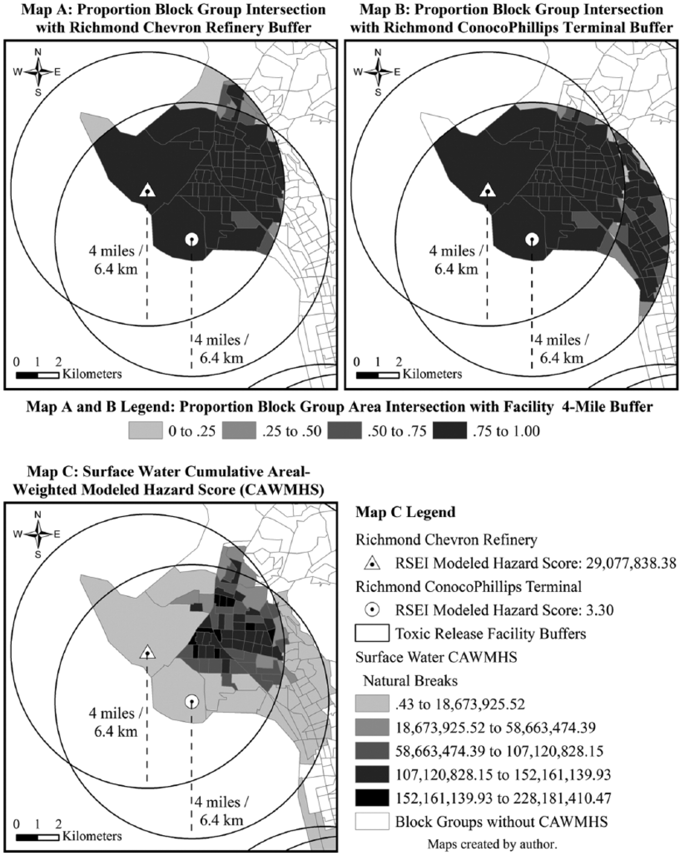
Illustration of CAWMHS methodology for surface water toxic releases in Richmond, California, 2000.

Figure 4.

Surface water CAWMHSs logged in the Bay-Delta, 2000.

Independent Variables

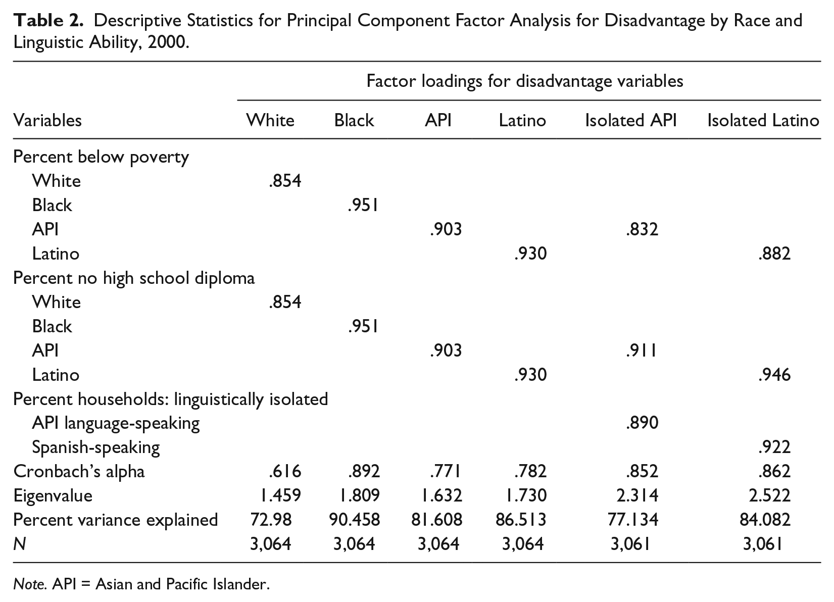
Following established practice in previous research (e.g., Grineski, Bolin, and Boone 2007; Grineski et al. 2010; Sicotte and Swanson 2007; Smith 2007), I use principal component factor analysis to reduce six sets of highly correlated variables from the 2000 census into separate explanatory factor variables. Doing so allows me to test the three intersectional hypotheses outlined above while avoiding problems of collinearity between the independent variables. Table 2 summarizes the results of the factor analysis. Each factor includes two dimensions of socioeconomic disadvantage disaggregated by race: the percent of individuals whose 1999 income was below poverty and the percent of individuals 25 years and older without a high school diploma that self-identify as white, black, API, and Latino.⁵ These two categories of socioeconomic disadvantage are limited in contrast to comparable categories used in previous research that do not distinguish socioeconomic status by race (e.g., Sicotte and Swanson 2007; Smith 2007). However, the poverty and education measures are suitable for the present study because poverty and educational attainment are important correlates of vulnerability of exposure to surface water hazards through subsistence fishing for various racial groups in the Bay-Delta (F. Shilling et al. 2010; Silver et al. 2007). I refer to socioeconomic disadvantage as simply “disadvantage” for each racial group below for brevity.

Table 2.

Descriptive Statistics for Principal Component Factor Analysis for Disadvantage by Race and Linguistic Ability, 2000.

Variables	Factor loadings for disadvantage variables
Variables	White	Black	API	Latino	Isolated API	Isolated Latino
Percent below poverty
White	.854
Black		.951
API			.903		.832
Latino				.930		.882
Percent no high school diploma
White	.854
Black		.951
API			.903		.911
Latino				.930		.946
Percent households: linguistically isolated
API language-speaking					.890
Spanish-speaking						.922
Cronbach’s alpha	.616	.892	.771	.782	.852	.862
Eigenvalue	1.459	1.809	1.632	1.730	2.314	2.522
Percent variance explained	72.98	90.458	81.608	86.513	77.134	84.082
N	3,064	3,064	3,064	3,064	3,061	3,061

Note. API = Asian and Pacific Islander.

The two additional factor variables shown in Table 2 include the racial group-specific measures of disadvantage, as well as the percent of households who are linguistically isolated and are either API language-speaking or Spanish-speaking. A “linguistically isolated household” is that in “which all members 14 years old and over speak a non-English language and also speak English less than ‘very well’ (have difficulty with English)” (U.S. Census Bureau 2002:B–32). The decision to include the respective linguistic isolation variable in the isolated API and Latino disadvantage factors was informed by the prevalence of non-English fish advisories in the region (see, for example, Figure 2). The decision was also informed by the established association in the region between limited English-speaking ability among low-income and low-educated APIs and Latinos and heightened risk of exposure to surface water toxins through subsistence fishing (Silver et al. 2007).

Statistics shown for all six factor variables in Table 2 suggest they reliably measure the respective analytical constructs of disadvantage and linguistic ability by race. The factors have eigenvalues greater than 1, Cronbach’s alpha scores greater than .600, and explain at least 72 percent of the variance in the component variables. The least reliable construct is white disadvantage. Isolated disadvantage factors for APIs and Latinos are the most reliable. Comparing the correlation structure of the component variables for the isolated API and Latino disadvantage factors suggests different and similar underlying drivers of vulnerability for each group. Isolated Latino disadvantage loads higher on all three of its components than is seen with the isolated API disadvantage factor, while both isolated disadvantage factors for APIs and Latinos load highest on percent no high school diploma and percent non-English-speaking, linguistically isolated households.

The control variables used in the regression analysis account for other correlates of residential proximity to environmental hazards and residential toxic hazard levels as suggested by previous research and/or the particularities of the Bay-Delta case. The first control is percent employed in manufacturing from the 2000 census. Previous research demonstrated this aggregate-level variable was positively associated with residential proximity to hazardous waste facilities across the United States (Anderton et al. 1994) and with residential proximity to air-toxic release facilities and air-toxicity levels in California (Pastor et al. 2005; Pastor et al. 2004). The relationship between local housing values and environmental hazard distribution is typically thought to be inverse, but it is not so clear based on recent nationwide analyses (Downey and Hawkins 2008; Liévanos 2015). I explored patterns in the data, followed Manuel Pastor et al. (2005) and Liévanos (2015), and found that the ratio of block group-to-county median housing values was consistently and negatively associated with block group surface water CAWMHS. Thus, I incorporated this control into the regression models.

Two other control measures pertain to land use and additional salient spatial dynamics of environmental hazard distribution in the Bay-Delta. Pastor et al. (2005) illustrated that percent of land use devoted to industry, commerce, or transportation derived from the U.S. Geological Survey National Land Cover Database (NLCD) is a positive predictor of proximate air-toxic concentrations. This land use classification is captured in v2.0 of the 2001 NLCD (U.S. Geological Survey 2011) as “high intensity development,” meaning land cover that has 80 to 100 percent impervious surface and is associated with “highly developed areas where people reside or work in high numbers,” such as “apartment complexes, row houses and commercial/industrial” (Homer et al. 2004:836). I extracted the spatial data representing this land use classification from the 2001 NLCD and intersected it with Bay-Delta block groups to produce a block group-level percent high intensity development. Following Pastor et al. (2005) and Liévanos (2015), I expect this variable to be positively associated with surface water CAWMHS. Finally, a spatial dynamic evident across Table 1 and Figures 3 and 4 is that many of the surface water toxic release facilities cluster near Richmond and the San Francisco Bay with the highest surface water CAWMHS values attributed to the Richmond Chevron Refinery. The final control variable—kilometers from block group centroid to the centroid of the Richmond Chevron Refinery—captures the independent block group vulnerability factor of spatial proximity to the Chevron Refinery. I expect this variable to be negatively associated with surface water CAWMHS.

Analytic Strategy

ArcGIS v10.2.2 was used for all spatial measurements in this analysis, while GeoDa v1.4.5 was used to run multivariate linear regression models to assess the association between the block group-level independent variables and logged surface water CAWMHS. My linear regression strategy followed the spatial econometric approaches established by Luc Anselin (2005) and as applied to environmental inequality studies of air- and land-based hazards by Pastor et al. (2005), Jayajit Chakraborty (2009), and Sara E. Grineski et al. (2010). Doing so entailed running an ordinary least squares (OLS) regression model of logged surface water CAWMHS on the explanatory and control variables to initially specify the linear model. However, OLS models are often inadequate for spatial data because the models’ residuals tend to violate the assumption that they are independent and randomly distributed across space. Indeed, Moran’s I tests revealed the residuals exhibited significantly positive spatial autocorrelation, which necessitated the use of the Lagrange Multiplier (LM) diagnostic test to determine which spatial regression model—the spatial lag or spatial error—was appropriate to address the spatial effects in the linear regression (Anselin 2005).

The spatial error model was the appropriate choice given its significant and relatively higher LM value than that for the spatial lag specification. Substantively, the spatial error model “assumes that regression errors are spatially dependent and that the included explanatory variables do not fully explain spatial autocorrelation” (Chakraborty 2009:683). Furthermore, ignoring the spatially correlated errors could result in “a problem of efficiency, in the sense that the OLS coefficient standard error estimates are biased, but the coefficient estimates themselves remain unbiased” (Anselin 2009:261). The spatial error model supplements the OLS regression equation by adding a spatially weighted error term $λ W e$ and it is estimated using a maximum likelihood method. This model is summarized as:

y = α + \sum_{k} β_{k} X_{k} + λ W e + u,

where y is the natural log of surface water CAWMHS, $α$ is the constant, and $β$ represents the coefficient for the k number of X explanatory and control variables, $λ$ is the spatial autoregressive coefficient, W is the spatial weights matrix, e is the random error term from the OLS model, and u signifies the spatially independent error term (Anselin 2005, 2009; Chakraborty 2009).

A spatial weights matrix specifying the spatial relationships between block groups was required for the spatial error modeling effort. Following earlier research, I experimented with various inverse, distance-based, row standardized spatial weights matrices given the irregularly shaped block groups and the distance-decaying relationships among the variables (Chakraborty 2009; Grineski et al. 2010; Pastor et al. 2005). I found spatial autocorrelation among the regression residuals ceased at 2,000 meters between block group centroids. This definition of the “neighborhood” resulted in a very low 2.80 percent (N = 30) of the 1,072 block groups included in the regression analysis that were designated as neighborless because their centroids were beyond the 2,000 meter threshold to a nearest neighbor. It also resulted in a maximum of 67 and mean of 23 neighbors across the remaining 97.20 percent (N = 1,042) block groups with a nearest neighbor. For consistency, I also use a 2,000-meter, inverse distance-based, row standardized spatial weight matrix for other spatial autocorrelation tests in this analysis.

Results

Block Groups by 50 Percent Areal Containment within Facility Buffers

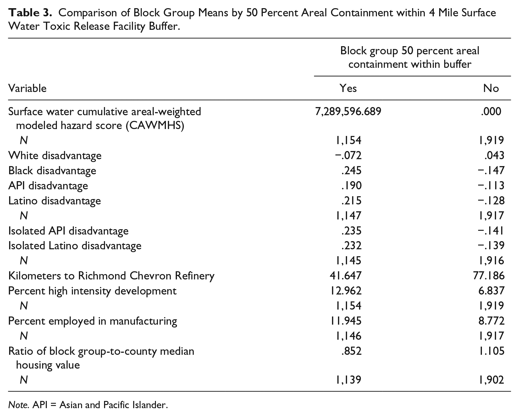
Table 3 displays the comparison of means for block groups by the extent to which they had 50 percent areal containment within the surface water toxic release facility buffers. The purpose of the table is to describe the average differences of block groups according to their 50 percent areal containment status before proceeding to the analysis of the multivariate determinants of surface water CAWMHS for block groups that met the 50 percent areal containment threshold.⁶ Table 3 reveals that block groups meeting that containment threshold have an average raw surface water CAWMHS of more than 7 million. Block groups outside that containment threshold do not have surface water CAWMHS.

Table 3.

Comparison of Block Group Means by 50 Percent Areal Containment within 4 Mile Surface Water Toxic Release Facility Buffer.

Variable	Block group 50 percent areal containment within buffer
Variable	Yes	No
Surface water cumulative areal-weighted modeled hazard score (CAWMHS)	7,289,596.689	.000
N	1,154	1,919
White disadvantage	−.072	.043
Black disadvantage	.245	−.147
API disadvantage	.190	−.113
Latino disadvantage	.215	−.128
N	1,147	1,917
Isolated API disadvantage	.235	−.141
Isolated Latino disadvantage	.232	−.139
N	1,145	1,916
Kilometers to Richmond Chevron Refinery	41.647	77.186
Percent high intensity development	12.962	6.837
N	1,154	1,919
Percent employed in manufacturing	11.945	8.772
N	1,146	1,917
Ratio of block group-to-county median housing value	.852	1.105
N	1,139	1,902

Note. API = Asian and Pacific Islander.

Also, as expected, block groups meeting the buffer containment threshold have dissimilar levels of disadvantage by race when compared with the block groups not meeting the containment threshold. On average, block groups contained within the facility buffers have .115 points lower levels of white disadvantage and have between .303 and .392 points higher levels of black, API, and Latino disadvantage, and isolated API and Latino disadvantage than block groups not contained in the facility buffers. Among the control variables used in the analysis, block groups contained in the facility buffers are, on average, more likely to be proximate to the Richmond Chevron Refinery, have higher percentage of workers employed in manufacturing, have higher percentage of high intensity development, and have lower median housing values than block groups not contained in the facility buffers.

Determinants of Surface Water CAWMHS

Table 4 provides descriptive statistics for the variables used in the spatial error regression models that test the three guiding hypotheses regarding the demographic determinants of surface water CAWMHS. The Moran’s I values shown in Table 4 reveal that all the variables exhibit significant positive spatial autocorrelation and thus are not randomly distributed across space. Such spatial clustering points to the high likelihood of spatial dynamics mediating the relationship between the independent variables and surface water CAWMHS, and it provides further justification for the spatial regression approach taken in this article. The high Moran’s I for logged surface water CAWMHS and kilometers to the Richmond Chevron Refinery are particularly noteworthy when considered in relation to Figures 3 and 4. Those patterns speak to the significant clustering of surface water CAWMHS near the Richmond Chevron Refinery and the importance of incorporating the additional spatial control of proximity to the refinery in the spatial regression analysis rather than relying strictly on the spatial autoregressive coefficient in the spatial error model to address the spatial processes affecting the relationship between block group attributes and surface water CAWMHS.

Table 4.

Descriptive Statistics for Surface Water CAWMHSs and Independent Variables Used in the Spatial Regression Analysis (N = 1,072).

Variable	M	SD	Minimum	Maximum	Moran’s I^a
Surface water CAWMHS logged	8.727	4.382	−.855	19.246	.887***
White disadvantage	−0.038	0.981	−1.289	6.166	.419***
Black disadvantage	0.283	1.288	−0.504	8.544	.542***
API disadvantage	0.183	1.113	−0.556	9.151	.336***
Latino disadvantage	0.247	1.201	−0.712	6.081	.592***
Isolated API disadvantage	0.210	1.164	−0.578	10.560	.362***
Isolated Latino disadvantage	0.274	1.227	−0.718	6.419	.572***
Km to Richmond Chevron Refinery	41.111	30.305	1.260	107.818	.960***
Percent employed in manufacturing	11.260	6.957	0.000	49.034	.445***
Percent high intensity development	13.298	17.203	0.000	94.183	.375***
Ratio of block group-to-county median housing value	0.828	0.400	0.061	3.426	.462***

Note. CAWMHS = cumulative areal-weighted modeled hazard score; API = Asian and Pacific Islander; Km = kilometer.

Based on 9,999 permutations and a 2,000-meter spatial weights matrix.

***

Pseudo p < .001 (two-tailed z test).

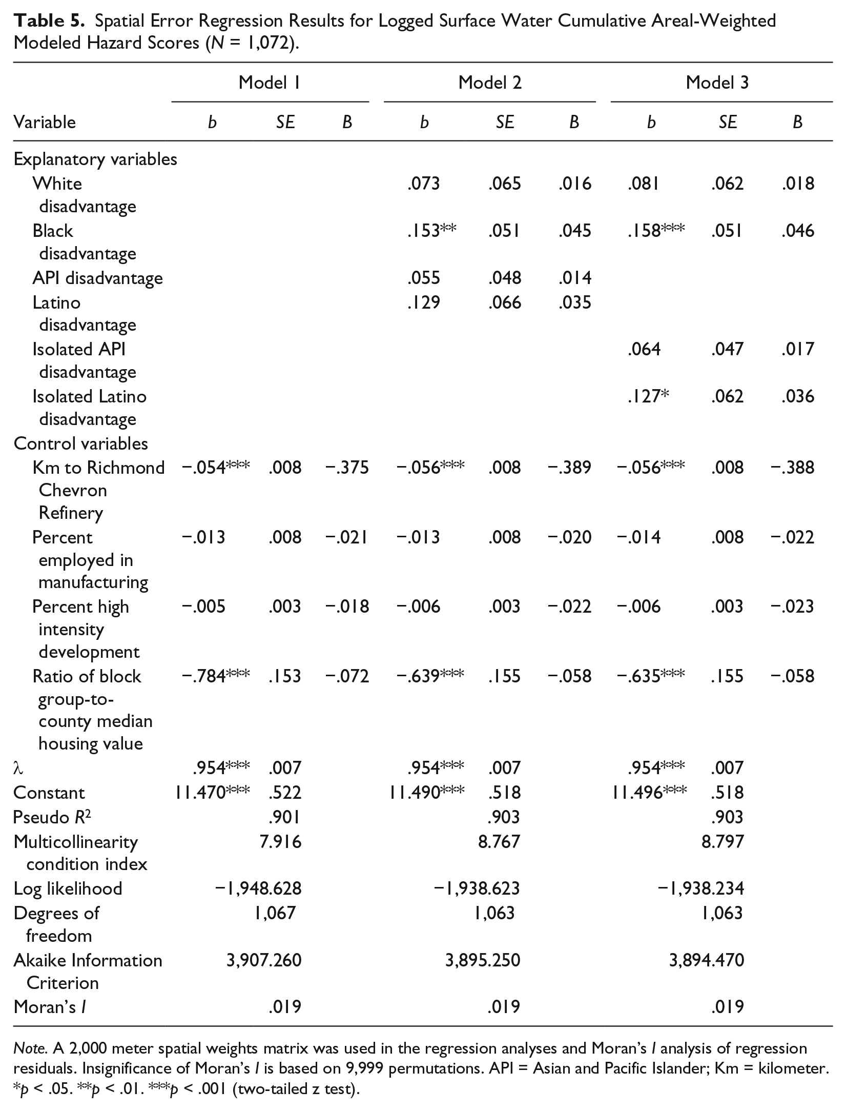
Table 5 reports the spatial error regression results for logged surface water CAWMHS. The modeling process summarized in the table adapts Liévanos’s (2015) intersectional approach to the demographic predictors of census tract presence in air-toxic clusters in the continental United States for the present study’s focus on the determinants of block group-level surface water CAWMHS in California’s Bay-Delta region. Model 1 establishes the effects of the control variables on logged surface water CAWMHS. The model reveals the coefficients for percent employed in manufacturing and percent high intensity development are negatively associated with logged surface water CAWMHS, but they are not significant. This pattern is manifest throughout the remainder of the regression analyses and counters previous research on the salience of percent manufacturing employment (Anderton et al. 1994) and of high intensity (i.e., urban-industrial) development (Liévanos 2015; Pastor et al. 2005) in determining environmental inequality outcomes. In contrast, the consistently significant and negative association between kilometers to the Richmond Chevron Refinery and the ratio of block group-to-county median housing values and logged surface water CAWMHS across all three models is as expected. Furthermore, the standardized regression coefficients for the Richmond Chevron Refinery proximity variable and relative median housing values throughout the analyses reveal they are the strongest two determinants of logged surface water CAWMHS among all of the variables included in the regression analyses.

Table 5.

Spatial Error Regression Results for Logged Surface Water Cumulative Areal-Weighted Modeled Hazard Scores (N = 1,072).

Variable	Model 1			Model 2			Model 3
Variable	b	SE	B	b	SE	B	b	SE	B
Explanatory variables
White disadvantage				.073	.065	.016	.081	.062	.018
Black disadvantage				.153**	.051	.045	.158***	.051	.046
API disadvantage				.055	.048	.014
Latino disadvantage				.129	.066	.035
Isolated API disadvantage							.064	.047	.017
Isolated Latino disadvantage							.127*	.062	.036
Control variables
Km to Richmond Chevron Refinery	−.054***	.008	−.375	−.056***	.008	−.389	−.056***	.008	−.388
Percent employed in manufacturing	−.013	.008	−.021	−.013	.008	−.020	−.014	.008	−.022
Percent high intensity development	−.005	.003	−.018	−.006	.003	−.022	−.006	.003	−.023
Ratio of block group-to-county median housing value	−.784***	.153	−.072	−.639***	.155	−.058	−.635***	.155	−.058
λ	.954***	.007		.954***	.007		.954***	.007
Constant	11.470***	.522		11.490***	.518		11.496***	.518
Pseudo R²	.901			.903			.903
Multicollinearity condition index	7.916			8.767			8.797
Log likelihood	−1,948.628			−1,938.623			−1,938.234
Degrees of freedom	1,067			1,063			1,063
Akaike Information Criterion	3,907.260			3,895.250			3,894.470
Moran’s I	.019			.019			.019

Note. A 2,000 meter spatial weights matrix was used in the regression analyses and Moran’s I analysis of regression residuals. Insignificance of Moran’s I is based on 9,999 permutations. API = Asian and Pacific Islander; Km = kilometer.

p < .05. **p < .01. ***p < .001 (two-tailed z test).

Models 2 and 3 test the dissimilar, nonwhite disadvantage, and black disadvantage water injustice hypotheses, net of controls. Model 2 adds the four disadvantage factors for whites, blacks, APIs, and Latinos, and model 3 replaces API and Latino disadvantage with isolated disadvantage factors for APIs and Latinos because these factors are collinear with API and Latino disadvantage. Thus, the primary difference between models 2 and 3 is the latter model incorporates linguistic isolation into the analysis of socioeconomic disadvantage by racial status for APIs and Latinos (cf. Liévanos 2015).

The diagnostics for the three spatial error models suggest they successfully address concerns over multicollinearity and spatial dependence. The multicollinearity condition indices for models 1, 2, and 3 vary between 7.916 and 8.797, are well below the suggested threshold of 30 (Anselin 2005), and therefore verify the lack of significant collinearity between the independent variables in each of the models. In addition, spatial dependence is not evident in these spatial error models as indicated by the highly statistically significant spatial autoregressive coefficient (Lamda; λ) in each model and the insignificant Moran’s I statistics for the spatial error residuals.

The pseudo R² for each model indicates the models account for about 90 percent of the variance explained in the logged surface water CAWMHS. The Akaike information criterion (AIC) and the log likelihood statistics are the preferred comparison metrics, as smaller AIC values and larger log likelihood values suggest improved model fit across competing models (Anselin 2005; Chakraborty 2009). In this case, models 2 and 3 are marginal improvements upon the control variables in model 1: the log likelihood increased by .51 percent in model 2 and by .53 percent in model 3, and the AIC decreased by .31 percent in model 2 and .33 percent in model 3.

The results presented for models 2 and 3 provide varying levels of support for the three hypotheses guiding this analysis. All six explanatory variables have dissimilar associations with logged surface water CAWMHS. However, only two explanatory variables are significant and positively associated with logged surface water CAWMHS: black disadvantage in models 2 and 3 and isolated Latino disadvantage in model 3. These patterns mean there is limited support for the dissimilar and nonwhite disadvantage water injustice hypotheses. These results also suggest there are different sociospatial dimensions of vulnerabilities of exposure to surface water CAWMHS for different racialized groups in the Bay-Delta region in the year 2000. Specifically, block group levels of white disadvantage, API disadvantage, and isolated API disadvantage were not significantly associated with logged surface water CAWMHS, net of other factors in the models.

In contrast, the results for the Latino factors indicate that intersecting axes of poverty, low educational attainment, and limited English proficiency and linguistic isolation for Latinos are the significant factors that create this racialized group’s block group-level vulnerability of exposure to surface water CAWMHS in the region. The unstandardized coefficient for isolated Latino disadvantage in model 3 signifies a one-unit increase in that factor is associated with a 12.7 percent increase in logged surface water CAWMHS, net of other factors in the model. Furthermore, the statistical significance of isolated Latino disadvantage and its standardized regression coefficient in model 3 indicates it is the fourth strongest significant determinant of logged surface water CAWMHS behind proximity to the Richmond Chevron Refinery, median housing values, and black disadvantage, net of other variables in the model. That standardized coefficient can be interpreted as a 1 standard deviation increase in isolated Latino disadvantage being significantly associated with a 3.6 percent increase in logged surface water CAWMHS.

The black disadvantage water injustice hypothesis is fully supported because black disadvantage is the strongest positive demographic determinant of logged surface water CAWMHS in models 2 and 3. This is indicated by the significance of this variable in the models and the magnitude of the standardized regression coefficient, the latter of which can be interpreted net of other factors as a 1 standard deviation increase in black disadvantage being significantly associated with, respectively, a 4.5 and 4.6 percent increase in logged surface water CAWMHS in model 2 and model 3. The unstandardized coefficient for black disadvantage suggests a 1-unit increase in black disadvantage is associated with a 15.3 percent increase in logged surface water CAWMHS in model 2 and is associated with a 15.8 percent increase in logged surface water CAWMHS in model 3. The regression analysis thus reveals the relatively durable and strong relationship between block group levels of black disadvantage and vulnerability of exposure to surface water CAWMHS in the Bay-Delta region.

There are marginal differences between models 1, 2, and 3 in the context of their diagnostic statistics. However, model 3 has the smallest AIC values and largest log likelihood values, which indicate it is the best fitting model in the analysis. Overall, the results from this model suggest that among all the variables included in the analysis, proximity to the Richmond Chevron Refinery, relatively low median housing values, black disadvantage, and isolated Latino disadvantage are the strongest determinants of block group-level modeled hazard levels for surface water toxic releases in California’s Bay-Delta in the year 2000.

Discussion and Conclusion

Environmental inequality and justice scholars have advanced our understanding of water injustice in the United States and abroad. Collectively, they have illuminated the wide array of environmental inequalities embedded in and produced by (1) institutional authorities’ misrecognition of diverse ways of managing societal-water relations, (2) procedural inequities in water governance, and (3) the unequal distribution of rights to access healthy and affordable water (Lu et al. 2014; Zwarteveen and Boelens 2014). This article charts a new research direction on the sociospatial dimensions of water injustice with a cross-sectional case study of the relationship between the modeled health hazards of proximate surface water toxic releases and the intersection of block group-level racial composition, socioeconomic disadvantage, and linguistic ability in California’s Bay-Delta region in 2000.

The spatial analytical techniques presented in this article advance a new approach to measuring the sociospatial dimensions of water injustice with the block group-level cumulative CAWMHS for surface water toxic releases. This new approach builds upon previous research in a number of ways. First, it incorporated Mohai and Saha’s (2007) 50 percent areal containment technique by determining which block groups had at least 50 percent of their area contained within the U.S. EPA-designated 4 mile/6.4 kilometer plausible exposure zone (Harner et al. 2002) to surface water toxic release facilities in California’s Bay-Delta. Second, building on Sicotte and Swanson (2007), the modeled hazard scores of surface toxic releases were extracted from the U.S. EPA RSEI database and distributed to block groups according to the proportion of their area that was contained in the buffer and whether they met the 50 percent areal containment threshold. The resulting areal-weighted modeled hazard scores were then summed for each block group to derive the surface water CAWMHS, which was then divided by the area of each block group to derive a hazard density measure akin to Bolin et al.’s (2002) cumulative hazard density index (CHDI). The CAWMHS thus adapts the CHDI in a manner that incorporates the health hazard data from the RSEI database specifically for surface water toxic releases and addresses calls from environmental inequality scholars (e.g., Chakraborty et al. 2011; Collins et al. 2011; Downey and Hawkins 2008; Liévanos 2015; Mohai et al. 2009; Pastor et al. 2005) to improve the measurement and understanding of environmental health hazards and their unequal distribution.

There are important caveats to the surface water CAWMHS. Specifically, it pertains only to toxic releases directly to surface waters from manufacturing facilities included in the U.S. EPA RSEI database. It therefore does not pertain to nonpoint sources (e.g., water pollution runoff), drinking water contaminants, or indirect water toxic release transfers to publicly owned treatment works. The measure also does not account for individual human exposures to and health impacts of surface water toxic releases. The surface water CAWMHS measure is also limited because it does not model the movement of surface water toxins through the environment as found in hydrological analyses used for assessing total maximum daily loads for U.S. waterways (e.g., Keisman and Shenk 2013; Ortolani 2014).

An alternative approach beyond the scope of the present study could use distance-decay modeling to assess the sociospatial dimensions of water injustice in the Bay-Delta region. This approach would conceptualize environmental inequality outcomes as continuous rather than discrete (Chakraborty et al. 2011; Downey 2006a, 2006b). That is, distance-decay modeling would permit a researcher to assess unequal surface water health hazard levels for proximate census geographies as a spatial phenomenon that declines as distance increases from each surface water toxic release facility throughout the entire study area. This alternative approach deviates from the present study’s understanding of water injustice and environmental inequality outcomes as discrete and bounded by the U.S. EPA designated 4 mile/6.4 kilometer plausible exposure zones. However, the surface water CAWMHS measure developed in the present study is successful in meeting its intended purpose of advancing our understanding of the sociospatial dimensions of water injustice by (1) rigorously and reliably identifying census block groups that face plausible exposures to toxicity- and proximity-weighted cumulative health hazards of surface water toxic releases, and (2) facilitating a cross-sectional assessment of the block group-level social and spatial attributes that are significantly associated with the estimated health hazards of proximate surface water toxic releases.

This article’s intersectional approach to water injustice represents its other major contribution to water injustice and environmental inequality outcomes research. The multivariate results reviewed above illuminate how different axes of social inequality for whites, blacks, APIs, and Latinos intersect and contribute to the sociospatial dimensions of block group-level vulnerability of exposure to health hazards of toxic releases emitted directly from manufacturing facilities to the surface waters of California’s Bay-Delta region in 2000. Net of proximity to the highest polluting facility in the region (i.e., the Richmond Chevron Refinery), housing values, and other factors considered in the analysis, block group levels of socioeconomically disadvantaged blacks and linguistically isolated and socioeconomically disadvantaged Latinos are the primary determinants of health hazard levels from proximate surface water toxic releases in the region. These findings regarding the sociospatial dimensions of water injustice in the region build upon previous research that identified population-level variables of poverty and low education attainment among blacks and poverty, low educational attainment, and limited English-speaking ability among Latinos as factors that shape vulnerability of exposure to air-toxic releases (Shah 2008) and surface water hazards through subsistence fishing and contaminated fish consumption in the Bay-Delta (F. Shilling et al. 2010; Silver et al. 2007). In addition, black disadvantage was a stronger demographic determinant of surface water CAWMHS among other comparable demographic factors, including isolated Latino disadvantage. That finding fully supports the black disadvantage water injustice hypothesis developed in this article, which posited the spatial concentration of socioeconomically disadvantaged blacks will be the strongest positive demographic determinant of modeled hazard levels of proximate surface water toxic releases.

The results for black disadvantage extend research on intersectional environmental inequality outcomes of aggregate-level air-toxic concentrations within the United States. Specifically, Downey and Hawkins’s (2008) nationwide, tract-level analysis found that low-income black areas are disproportionately associated with cumulative air-toxic releases from manufacturing facilities in 2000. Likewise, Liévanos’s (2015) nationwide, tract-level analysis of 2000 demographic data and 2005 air-toxic lifetime cancer risk data found the concentration of economically deprived blacks was among the strongest demographic predictors of census tract location in 2005 air-toxic lifetime cancer risk clusters. The present study’s findings regarding the disproportionately strong, positive, and significant association between block group levels of socioeconomically disadvantaged blacks and modeled health hazards of proximate surface water toxic releases in California’s Bay-Delta suggest that nearby surface waters are yet another environmentally hazardous context for socioeconomically marginalized black residential settlements in the United States. Such context has hitherto gone unnoticed in previous environmental inequality research (Chakraborty et al. 2011) and is missing from urban sociological accounts on the plight of the “truly disadvantaged,” black residential settlements of the United States (Marcuse 1997; Wacquant 2008; Wilson 1987).

The results for isolated Latino disadvantage also build upon on intersectional environmental inequality outcomes research pertaining to aggregate-level air-toxic concentrations within the United States. Collins et al.’s (2011) analysis of the relationship between block group-level 2000 census population and housing data and 2002 estimated lifetime cancer risk from air-toxic concentrations in El Paso County, Texas, found that poverty and low educational attainment for Latinos and Spanish-speaking households with limited English-language proficiency were disproportionately associated with air-toxic cancer risk levels. Liévanos (2015) found that a factor variable representing Spanish-speaking, linguistically isolated, and economically deprived Latino immigrants was the strongest positive demographic predictor of census tract location in 2005 air-toxic lifetime cancer risk clusters in the continental United States. The present study’s finding regarding isolated Latino disadvantage extends Collins et al.’s (2011) and Liévanos’s (2015) insights into the water environment of the California Bay-Delta. Furthermore, when contrasted with the nonsignificant effect of Latino disadvantage versus the significant effect of isolated Latino disadvantage on surface water CAWMHS, the present study provides further evidence that attending solely to the intersection of race and class in environmental inequality outcomes neglects the contingent ways in which multiple axes of social inequality, particularly linguistic ability, shape environmental inequalities in Latino residential settlements in the United States.

Future research could build on the results from the present study in a number of ways. For example, the methods deployed in this article could be replicated and compared against distance-decay approaches, as described above, for census geographies throughout the entire United States to derive nationwide estimates of localized water injustices associated with surface water toxic releases. Such analyses could set the stage for comparative analyses of water injustice across a greater expanse of block groups, tracts, cities, and regions. Fruitful cross-case analyses could illuminate how historical forces (e.g., racial segregation and uneven development) may contribute to the water injustices documented in the present study and possibly in other comparably impaired and socially unequal regions such as the Chesapeake Bay, the Columbia River Basin, the Florida Everglades, and the Mississippi River Delta (Heikkila and Gerlak 2005). Furthermore, researchers could replicate the CAWMHS measures for air- and land-based toxic releases and combine the results with those for surface water toxic releases and other water-based measures found in the U.S. EPA RSEI database to get a better sense of the cumulative health hazard of toxic releases in the United States.

Lastly, there are important practical implications of the present study for environmental justice policy in California’s Bay-Delta. Silver et al. (2007) have argued that multilingual environmental health risk advisories and outreach and education efforts may be important ways to lower exposure to surface water toxins through fish consumption for vulnerable populations in the region. In contrast, water justice advocates argue that such efforts are incomplete without targeted land use reform and environmental justice policies that, at minimum, channel industrial land uses away from local waterways and lower the excessive amounts of toxic releases into the watershed (Vanderwarker 2006). The present study suggests the hazardous spaces near the Richmond Chevron Refinery and other residential settlements comprised of marginalized blacks and Latinos are important starting points for such reforms in the region.

Footnotes

Acknowledgements

I thank Don Dillman, Emily Huddart Kennedy, Tom Rotolo, Monica Johnson, Jennifer Givens, Christine Horne, Clay Mosher, Katrina Leupp, Alair MacLean and anonymous reviewers for helpful comments on earlier drafts of this article. I accept full responsibility for any errors or omissions in this article.

Declaration of Conflicting Interests

The author(s) declared no potential conflicts of interest with respect to the research, authorship, and/or publication of this article.

Funding

The author(s) disclosed receipt of the following financial support for the research, authorship, and/or publication of this article: Funding for this research was provided in part by the Ford Foundation, the Rose Foundation, the University of California (UC) Berkeley Community Forestry and Environmental Research Partnerships Program, UC Davis Atmospheric Aerosols and Health Program, UC Davis Center for Regional Change, UC Davis Department of Sociology, UC Davis John Muir Institute of the Environment: Environmental Justice Project, UC Toxic Substances Research and Teaching Program, and the Washington State University Department of Sociology.

Notes

Author Biography

Raoul S. Liévanos is an assistant professor of sociology at the University of Oregon. His scholarly interests are in environmental and urban sociology; race and ethnicity; social movements, organizations, and institutions; geographic information systems and spatial analysis; qualitative field methods; and historical-comparative sociology. His primary research focuses on environmental and housing market inequalities and social movements and policy processes attempting to address such inequalities in the United States.

References

Anderton

Douglas L.

Anderson

Andy B.

Oakes

John Michael

Fraser

Michael R.

1994. “Environmental Equity: The Demographics of Dumping.” Demography 31:229–48.

Anselin

Luc

. 2005. Exploring Spatial Data with GeoDa™: A Workbook. Urbana, IL: University of Illinois. Retrieved April 21, 2016 (http://www.csiss.org/clearinghouse/GeoDa/geodaworkbook.pdf).

Anselin

Luc

. 2009. “Spatial Regression.” Pp. 255–75 in The SAGE Handbook of Spatial Analysis, edited by Fotheringham

A. S.

Rogerson

P. A.

Los Angeles, CA: Sage Publications.

Bolin

Bob

Nelson

Amy

Hackett

Edward J.

Pijawka

K. David

Smith

C. Scott

Sicotte

Diane

Sadalla

Edward K.

Matranga

Eric

O’Donnel

Maureen

. 2002. “The Ecology of Technological Risk in a Sunbelt City.” Environment and Planning A 34:317–39.

Brown

Phil

. 2007. Toxic Exposures: Contested Illnesses and the Environmental Health Movement. New York: Columbia University Press.

Chakraborty

Jayajit

. 2009. “Automobiles, Air Toxics, and Adverse Health Risks: Environmental Inequities in Tampa Bay, Florida.” Annals of the Association of American Geographers 99(4):674–97.

Chakraborty

Jayajit

Maantay

Juliana A.

Brender

Jean D.

2011. “Disproportionate Proximity to Environmental Health Hazards: Methods, Models, and Measurement.” American Journal of Public Health 101(S1):S27–S36.

Cole

Luke W.

Foster

Sheila R.

2001. From the Ground Up: Environmental Racism and the Rise of the Environmental Justice Movement. New York: New York University Press.

Collins

Timothy W.

Grineski

Sara E.

Chakraborty

Jayajit

McDonald

Yolanda J.

2011. “Understanding Environmental Health Inequalities through Comparative Intracategorical Analysis: Racial/Ethnic Disparities in Cancer Risks from Air Toxics in El Paso County, Texas.” Health & Place 17:335–44.

10.

Crowder

Kyle

Downey

Liam

. 2010. “Interneighborhood Migration, Race, and Environmental Hazards: Modeling Microlevel Processes of Environmental Inequality.” American Journal of Sociology 115(4):1110–149.

11.

Downey

Liam

. 2006a. “Environmental Racial Inequality in Detroit.” Social Forces 85(2):771–96.

12.

Downey

Liam

. 2006b. “Using Geographic Information Systems to Reconceptualize Spatial Relationships and Ecological Context.” American Journal of Sociology 112(2):567–612.

13.

Downey

Liam

Hawkins

Brian

. 2008. “Race, Income, and Environmental Inequality in the United States.” Sociological Perspectives 51(4):759–81.

14.

Environmental Justice Coalition for Water (EJCW). 2005. Thirsty for Justice: A People’s Blueprint for California Water. Oakland, CA: Environmental Justice Coalition for Water.

15.

Grineski

Sara E.

Bolin

Bob

Boone

Christopher

. 2007. “Criteria Air Pollution and Marginalized Populations: Environmental Inequity in Metropolitan Phoenix, Arizona.” Social Science Quarterly 88(2):535–54.

16.

Grineski

Sara E.

Collins

Timothy W.

Aguilar

María de Lourdes Romo

Aldouri

Raed

. 2010. “No Safe Place: Environmental Hazards & Injustice along Mexico’s Northern Border.” Social Forces 88(5):2241–266.

17.

Harner

John

Warner

Kee

Pierce

John

Huber

Tom

. 2002. “Urban Environmental Justice Indices.” The Professional Geographer 54(3):318–31.

18.

Heikkila

Tanya

Gerlak

Andrea K.

2005. “The Formation of Large-scale Collaborative Resource Management Institutions: Clarifying the Roles of Stakeholders, Science, and Institutions.” The Policy Studies Journal 33(4):583–612.

19.

Hernandez

Jesus

. 2009. “Redlining Revisited: Mortgage Lending Patterns in Sacramento 1930–2004.” International Journal of Urban and Regional Research 33(2):291–313.

20.

Homer

Collin

Huang

Chengquan

Yang

Limin

Wylie

Bruce

Coan

Michael

. 2004. “Development of a 2001 National Land Cover Database for the United States.” Photogrammetric Engineering & Remote Sensing 70(7):829–40.

21.

Keisman

Jeni

Shenk

Gary

. 2013. “Total Maximum Daily Load Criteria Assessment Using Monitoring and Modeling Data.” Journal of the American Water Resources Association 49(5):1134–149.

22.

Liévanos

Raoul S.

2013. “Cumulative Impact: Organizing Risk and the New Urban-environmental Crisis in Stockton, California.” PhD dissertation, Department of Sociology, University of California, Davis, Davis, CA.

23.

Liévanos

Raoul S.

2015. “Race, Deprivation, and Immigrant Isolation: The Spatial Demography of Air-toxic Clusters in the Continental United States.” Social Science Research 54:50–67.

24.

Flora

Ocampo-Raeder

Constanza

Crow

Ben

. 2014. “Equitable Water Governance: Future Directions in the Understanding and Analysis of Water Inequities in the Global South.” Water International 39(2):129–42.

25.

Marcuse

Peter

. 1997. “The Enclave, the Citadel, and the Ghetto: What Has Changed in the Post-Fordist U.S. City.” Urban Affairs Review 33:228–64.

26.

Massey

Douglass S.

Denton

Nancy A.

1993. American Apartheid: Segregation and the Making of the Underclass. Cambridge, MA: Harvard University Press.

27.

McClintock

Nathan

. 2011. “From Industrial Garden to Food Desert: Demarcated Devaluation in the Flatlands of Oakland, California.” Pp. 89–120 in Cultivating Food Justice: Race, Class, and Sustainability, edited by Alkon

A. H.

Agyeman

Cambridge, MA: MIT Press.

28.

Minnesota Population Center. 2004. National Historical Geographic Information System: Pre-release Version 0.1. Minneapolis, MN: University of Minnesota.

29.

Mohai

Paul

Pellow

David

Roberts

J. Timmons

. 2009. “Environmental Justice.” Annual Review of Environmental Resources 34:405–30.

30.

Mohai

Paul

Saha

Robin

. 2007. “Racial Inequality in the Distribution of Hazardous Waste: A National-level Reassessment.” Social Problems 54(3):343–70.

31.

Mohai

Paul

Saha

Robin

. 2015. “Which Came First, People or Pollution? A Review of Theory and Evidence from Longitudinal Environmental Justice Studies.” Environmental Research Letters 10(12):1–9.

32.

Ortolani

Vincent

. 2014. “Land Use and Its Effects on Water Quality Using the BASINS Model.” Environmental Earth Sciences 71(5):2059–2063.

33.

Pastor

Manuel

Morello-Frosch

Rachel

Sadd

James L.

2005. “The Air is Always Cleaner on the Other Side: Race, Space, and Ambient Air Toxics Exposures in California.” Journal of Urban Affairs 27(2):127–48.

34.

Pastor

Manuel

Sadd

James L.

Morello-Frosch

Rachel

. 2004. “Waiting to Inhale: The Demographics of Toxic Air Release Facilities in 21st-century California.” Social Science Quarterly 85(2):420–40.

35.

Pulido

Laura

. 1996. Environmentalism and Economic Justice: Two Chicano Struggles in the Southwest. Tucson, AZ: University of Arizona Press.

36.

Pulido

Laura

. 2000. “Rethinking Environmental Racism: White Privilege and Urban Development in Southern California.” Annals of the Association of American Geographers 90(1):12–40.

37.

Ringquist

Evan J.

2005. “Assessing Evidence of Environmental Inequities: A Meta-analysis.” Journal of Policy Analysis and Management 24(2):223–47.

38.

Robinson

Joanna L.

2013. Contested Water: The Struggle Against Water Privatization in the United States and Canada. Cambridge, MA: MIT Press.

39.

Shah

Bindi

. 2008. “‘Is Yellow Black or White?’ Inter-minority Relations and the Prospects for Cross-racial Coalitions between Laotians and African Americans in the San Francisco Bay Area.” Ethnicities 8(4):463–91.

40.

Shilling

Fraser

White

Aubrey

Lippert

Lucas

Lubell

Mark

. 2010. “Contaminated Fish Consumption in California’s Central Valley Delta.” Environmental Research 110:334–44.

41.

Shilling

Fraser M.

London

Jonathan K.

Liévanos

Raoul S.

2009. “Marginalization by Collaboration: Environmental Justice as a Third Party in and beyond CALFED.” Environmental Science & Policy 12(6):694–709.

42.

Sicotte

Diane

Swanson

Samatha

. 2007. “Whose Risk in Philadelphia? Proximity to Unequally Hazardous Industrial Facilities.” Social Science Quarterly 88(2):515–34.

43.

Silver

Elana

Kaslow

Jessica

Lee

Diana

Lee

Sun

Tan

May Lynn

Weis

Erica

Ujihara

Alyce

. 2007. “Fish Consumption and Advisory Awareness among Low-income Women in California’s Sacramento-San Joaquin Delta.” Environmental Research 104:410–19.

44.

Smith

Chad L.

2007. “Economic Deprivation and Environmental Inequality in Postindustrial Detroit: A Comparison of Landfill and Superfund Site Locations.” Organization & Environment 20(1):25–43.

45.

State Water Resources Control Board (SWRCB). 2008a. Geographic Information System (GIS) Shapefiles for 2006 303(d) List of Water Quality Limited Segments. Electronic datafile. Sacramento, CA: State Water Resources Control Board. Retrieved September 10, 2008 (http://www.waterboards.ca.gov/water_issues/programs/tmdl/docs/303dlists2006/gis/all303d_06_stwde.zip).

46.

State Water Resources Control Board (SWRCB). 2008b. List of Water Quality Limited Segments—All Portions. Electronic datafile. Sacramento, CA: State Water Resources Control Board. Retrieved September 10, 2008 (http://www.waterboards.ca.gov/water_issues/programs/tmdl/docs/303dlists2006/gis/state_06_303d_combined_wcat_rev.xls).

47.

Swyngedouw

Erik

. 2014. “Reply to the Santa Cruz Declaration on the Global Water Crisis—From Water Justice to Eco-political Equality: Politicizing Water.” Water International 39(2):258–59.

48.

Sze

Julie

London

Jonathan

Shilling

Fraser

Gambirazzio

Gerardo

Filan

Trina

Cadenasso

Mary

. 2009. “Defining and Contesting Environmental Justice: Socio-natures and the Politics of Scale in the Delta.” Antipode 41(4):807–43.

49.

U.S. Census Bureau. 2002. Technical Documentation: Census 2000 Summary File 3. Washington, DC: U.S. Census Bureau.

50.

U.S. Environmental Protection Agency (U.S. EPA). 2010a. EPA—Envirofacts—Geospatial Data Download—November 2010. Washington, DC: U.S. Environmental Protection Agency.

51.

U.S. Environmental Protection Agency (U.S. EPA). 2010b. User’s Manual for RSEI Version 2.3.0. Washington, DC: U.S. Environmental Protection Agency Office of Pollution Prevention and Toxics.

52.

U.S. Environmental Protection Agency (U.S. EPA). 2015. “Office of Water Fish Consumption Advisories.” Electronic datafile. Retrieved October 1, 2015 (https://edg.epa.gov/clipship/).

53.

U.S. Geological Survey. 2011. NLCD 2001 Land Cover Version 2.0. Sioux Falls, SD: U.S. Geological Survey.

54.

Vanderwarker

Amy

. 2006. “Water, Environmental Justice, and Land Use Planning: Richmond, California.” Progressive Planning 169(Fall):26–29.

55.

Wacquant

Loïc J. D.

2008. Urban Outcasts: A Comparative Sociology of Advanced Marginality. Malden, MA: Polity Press.

56.

Wilson

William Julius

. 1987. The Truly Disadvantaged: The Inner-city, the Underclass, and Public Policy. Chicago, IL: University of Chicago Press.

57.

Wilson

William Julius

. 1996. When Work Disappears: The World of the New Urban Poor. New York: Alfred A. Knopf.

58.

Zwarteveen

Margreet Z.

Boelens

Rutgerd

. 2014. “Defining, Researching, and Struggling for Water Justice: Some Conceptual Building Blocks for Research and Action.” Water International 39(2):143–58.