The Mobilizing Effects of Economic Threats and Resources on the Formation of Local Occupy Wall Street Protest Groups in 2011

Abstract

This paper examines how threatening economic conditions and preexisting community resources facilitated the spread of Occupy Wall Street protest groups to more than 600 counties in the continental United States in 2011. Using a generalized linear mixed model, we find that economic threats and accessible resources are complementary facilitators of movement mobilization. But contrary to the expectations based on earlier media and scholarly accounts, the “disruptive threats” caused by the Great Recession failed to predict the formation of Occupy groups. Instead, groups were more likely to mobilize in counties that had the “positional threats” of relatively higher income inequality and relatively lower median incomes in comparison to state norms. However, the effect of positional economic threats was nuanced as counties with lower than average unemployment more likely had groups mobilized. In addition, resources continue to demonstrate empirical importance in explanations of social movement mobilization, as Occupy groups were more likely to form in counties with greater access to social-organizational and human resources. Combined, these findings suggest that scholars can strengthen their analyses by considering threats and resources as complementary facilitators of local protest mobilization and by focusing greater attention on how differing types of threats may influence the mobilization of social movements.

Keywords

social movements threat resources Occupy Wall Street protest

On September 17, 2011, as many as 2,000 activists took possession of Zuccotti Park, two blocks from Wall Street in the center of Manhattan’s financial district (Schneider 2013). In the subsequent two-month period, Occupy Wall Street (OWS) groups mobilized in at least 1,000 towns and cities worldwide (Gould-Wartofsky 2015) with more than 600 groups forming in the continental United States (see Figure 1). The U.S. protesters’ demands were as varied as their locales. They included repealing the Citizens United decision, getting big money out of politics, reinstating the Glass-Stegall Act, ending foreclosures, reversing austerity policies, and increasing taxes on the wealthiest Americans (Schneider 2013). These sweeping demands were united under broad claims that economic and social advantages were not presently enjoyed by a majority of Americans (Gould-Wartofsky 2015; Schneider 2013).

Figure 1.

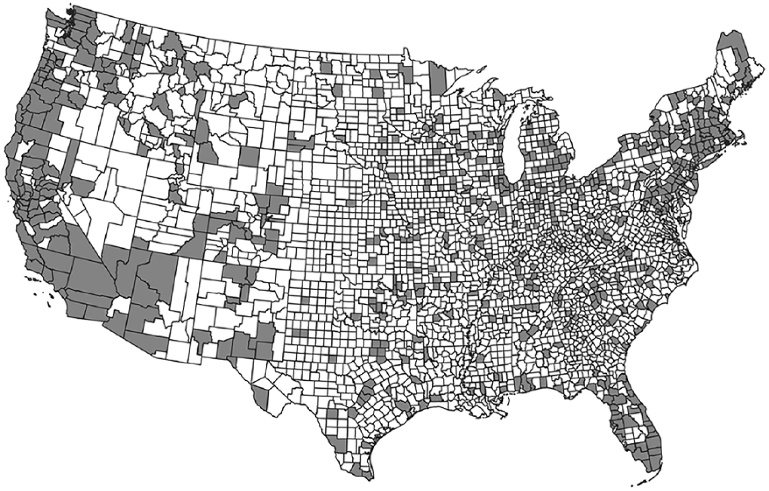
United States counties with occupy groups (in gray), 2011.

Popular interpretations at the time explained the emergence of the OWS protests as a reaction to the economic turmoil caused by the financial crisis and the subsequent recession. According to this account, job losses, declining incomes, and rising inequality fueled public aggravations, spurring protesters to mobilize in communities nationwide. This narrative was especially prominent in early media reporting on the Occupy movement (e.g., Kleinfield and Buckley 2011) and to a lesser degree is found in early scholarly accounts (e.g., Gould-Wartofsky 2015; Juris 2012; Lubin 2012; McVeigh 2011).¹ Yet, how well does this interpretation of the origins of OWS explain where groups mobilized in locales across the United States during the closing months of 2011? We contend that these conventional interpretations blur the distinction between two types of economic threats exacerbated by the economic downturn. We make a conceptual distinction between the disruptive and positional economic threats posed by the effects of the Great Recession. By “disruptive economic threats,” we mean those economic conditions that threatened the everyday material interests of people within a locale, such as increasing rates of unemployment, declining household incomes, and increasing levels of income inequality. In contrast, “positional economic threats” are those economic conditions that reflect the economic standing of people in a locality in comparison to other localities, such as higher rates of unemployment, lower household incomes, and higher levels of income inequality compared with state norms.

The findings indicate that the popular view of OWS’s emergence overlooks the distinction between these types of economic threats as well as the local variations in the availability of relevant human and organizational resources that facilitate protest mobilization. We show that, contrary to initial media and scholarly accounts, increasingly disruptive economic conditions within a locale generally failed to predict OWS protest mobilizations at the local level. Instead, those localities with economic positions worse than their state average, and with larger populations of college-educated residents and preexisting organizational resources, were more likely to mobilize OWS groups.

Our research makes two important contributions to scholarship. First, it differentiates between disruptive and positional threats to assess their respective roles in explaining patterns of local protest mobilization. Second, it affirms the salience of organizational and human resources but suggests that some were more important than others for the formation of OWS groups. Combined, these findings further demonstrate that threatening conditions and local mobilization capacity are complementary facilitators of movement mobilization.

Theoretical Background

Economic Threats and Social Movement Mobilization

The role of socioeconomic loss, or the threat of that loss, in explaining the emergence of social movements, is a subject of long-standing theoretical interest (see Goldstone and Tilly 2001; Opp 1988; Tilly 1978). The idea that protest groups mobilize to defend against perceived threats to social and material interests has also received empirical support, with most of this work focused on threats posed by declines in economic conditions (Caren, Gaby, and Herrold 2016; van Dyke and Soule 2002). We refer to these types of threatening conditions as “disruptive.” Another strand of research emphasizes that perceptions of economic threat are the product of comparative social assessments, and that the uneven distribution of socioeconomic conditions facilitates mobilization (McVeigh et al. 2014; Ward 2017). We refer to these types of threatening conditions as “positional.” The difference between the two types of threat is nuanced, but conceptually and analytically distinct.²

Disruptive economic threats and OWS

Prior research on the relationship between threatening conditions and mobilization focuses on those conditions that disrupt patterns of everyday life. This scholarship is centered on the idea that people are particularly averse to experiencing losses and will, therefore, be more open to “risk-seeking” behavior, like social movement participation, to protect against these losses (Kahneman and Tversky 1979). A generation of mostly case-study research documents how institutional and organizational actors may mobilize communities in reaction to threats, such as the citing of locally unwanted land-uses and environmental disasters (Bullard 2000; Edwards 1995; McGurty 2009). In one influential example, Edward Walsh (1981) concludes that the sudden imposition of grievances following the accident at the Three Mile Island nuclear reactor helped facilitate public protest against the facility. However, David A. Snow et al. (1998) point out that collective responses come not only from reactions to the suddenness of threats but also from the disruptions caused to daily routines. Similarly, we argue that economic threats associated with the Great Recession could have disrupted peoples’ lives over time, which contributed to the mobilization of local OWS groups nationally.

At the end of 2007, just as the recession was beginning, the national unemployment rate was at a low 5.0 percent (U.S. Department of Labor 2016). In the immediate months after the onset of the financial crisis, the economy began shedding hundreds of thousands of jobs a month (Goodman and Mance 2011). By August 2011, just weeks before OWS emerged in New York City, millions of people had lost their jobs, and the national unemployment rate stood at 9.0 percent (U.S. Department of Labor 2016). Over the same time period, the national median household income continued to decline and income inequality had increased (Federal Reserve Economic Data 2015; U.S. Census Bureau 2007, 2011a).³ Such national trends, however, mask the substantial local variation in the disruptive threats that we explore in our analysis. For example, in Mountrail County, North Dakota unemployment rates went from 5.7 percent in 2007 to 2.4 percent in 2011, which was a net decrease of 3.3 percentage points. In comparison, in Yuma County, Arizona unemployment rates went from 13.5 percent in 2007 to 26.8 percent in 2011, which was a net increase of 13.3 percentage points (U.S. Department of Agriculture 2014). This indicates that localities were differently impacted by the recession over time. Similar variations in local household income and income inequality occurred across the country during the time period (see Table 1 above).

Table 1.

Descriptive Statistics for County-level Variables (N = 3,106).

Variables	M	SD	Minimum	Maximum
Disruptive economic threats (2007–2011)
Unemployment rate change	3.68	1.90	−3.30	13.30
Median household income change	−2,136.48	3,040.13	−15,698.35	17,324.74
Income inequality change	0.23	1.87	−14.97	11.23
Positional economic threats (2011)
Unemployment rate relative to state mean	0.00	2.02	−6.07	16.23
Median household income relative to state mean	0.00	9,338.80	−28,604.58	71,842.76
Income inequality relative to state mean	0.00	3.21	−24.49	20.66
Social-organizational resources^a
Religious organization density	9.49	5.17	0.00	46.37
Civic organization density	1.27	1.59	0.00	19.31
Labor organization density	0.38	0.59	0.00	8.76
Political organization density	0.04	0.20	0.00	3.67
Human resources
Percent voted Obama in 2008	41.51	13.85	4.91	92.50
Percent college enrolled	5.27	4.02	0.00	52.01
Controls
Percent white	84.25	16.12	3.60	100
Population	99,447.8	317,710.6	95	9,888,476
Population density	260.46	1,750.27	0.14	70,500.79
State capital^b	—	—	—	—

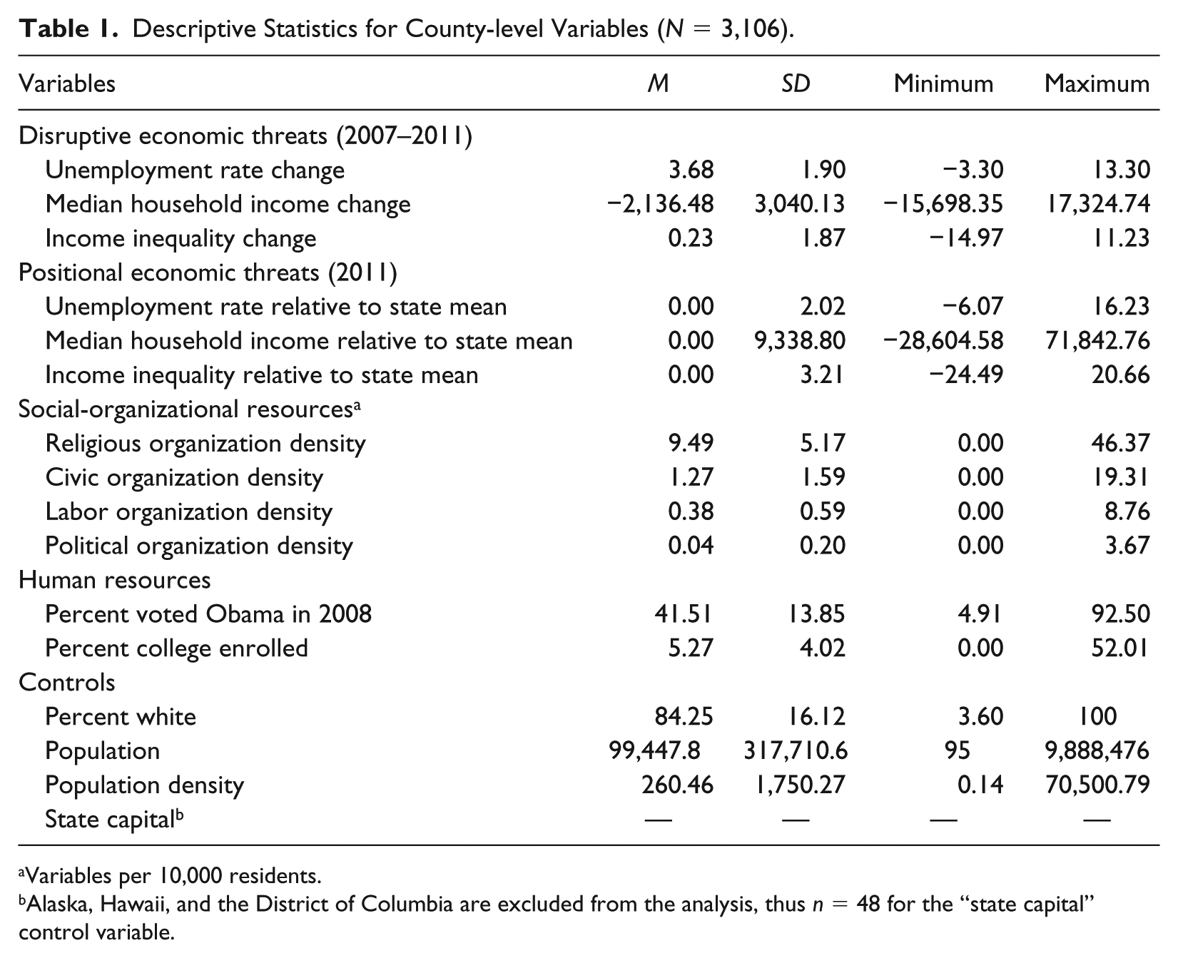
Variables per 10,000 residents.

Alaska, Hawaii, and the District of Columbia are excluded from the analysis, thus n = 48 for the “state capital” control variable.

In the analysis to follow, we focus on the extent to which local variability in the intensification of three disruptive economic threats—rising unemployment, declining household income, and rising income inequality—between 2007 and 2011 are associated with the formation of local OWS groups. These declining economic conditions, however, do not tell the full story of the threats encountered. People do not just evaluate threat in disruptive terms; they also evaluate threat through comparisons of social position as discussed below.

Positional economic threats and OWS

Our argument that economic threat can be understood in terms of a position in comparison to others draws from earlier social evaluation theories and more recent distributional theories. Social evaluation theorists argued that people compare themselves with reference groups to gauge their relative standing in economic and prestige hierarchies (Pettigrew 1967). Research in this tradition focused on how individuals who evaluated their relative positions negatively experienced deprivation and were subsequently more likely to engage in protest (e.g., Smelser 1962; Turner and Killian 1972). For its critics (e.g., Jenkins and Perrow 1977; McAdam 1982; McCarthy and Zald 1977), such “classical” or “grievance-based” theories had, at times, reduced social insurgency to a psychological phenomenon. Scholars critical of grievance-based theories viewed threats as diminishing a social movement’s chance to mobilize by decreasing access to the essential resources and opportunities that allow them to flourish (McAdam 1996; McAdam, Tarrow, and Tilly 1996). Others have argued, however, that the threat of current or anticipated harms do not work along a singular dimension to reduce movement mobilization (see Goldstone and Tilly 2001). From this view, a group may engage in social action, even if resources and opportunities are in decline, if the costs of not acting are perceived to worsen their collective lot.

Contemporary scholarship on distributive justice and spatial inequality recognize the power of social comparison at the aggregate level (see Jasso 2001; Lobao, Hooks, and Tickamyer 2007; McVeigh et al. 2014). Rather than conceptualize understandings of “fair” and “just” as simply intrapsychic processes tied to the experience of relative deprivation, macro-level work on the distribution of economic resources argues that collective assessments of “fairness” and “justness” are shaped by, and only make sense within, consensual structural contexts (Liebig and Sauer 2016). In other words, these shared judgments are influenced by external conditions that reflect the uneven distribution of advantages. This argument implies that patterned differentials in economic position are viewed as threatening because they indicate salient cleavages in society concerning the benefits and opportunities accessible to advantaged over disadvantaged populations. Following this work, we argue that common recognition of such positional threats affects social behaviors, including involvement in protests.

Applied to our case, the effects of the recession can not only be seen in the economic disruptions caused to locales from 2007 to 2011, it can also be seen in their resulting economic positions in 2011. Such threats to economic position are evident in the uneven standing of counties within their respective states, with some localities faring comparatively better and others worse. For example, in 2011, the unemployment rate in Marin County, California was 7.4 percent, which was 6.1 percentage points lower than the statewide average. In comparison, the unemployment rate in Kings County, California was 16.2 percent, which was 2.7 percentage points higher than the statewide average (U.S. Department of Agriculture 2014). Thus, residents living in Kings County may have questioned why they were in a much worse employment position than the residents in Marin County or elsewhere in their state. Similar variations in unemployment rates extended across the nation. As indicated in Table 1, these patterns of economic threat linked to the position of counties within their respective states also existed nationwide in terms of lower than average median household income and higher than average income inequality.

In the analysis below, we examine the degree to which local variability in the distribution of three positional economic threats—higher rates of unemployment, lower median household incomes, and higher levels of income inequality—between counties and their states in 2011 are associated with the formation of local OWS groups.

Given the difference between disruptive and positional economic threats conceptualized here, we expect each type of threat to exert an independent and positive influence on the likelihood of local OWS group formation. Therefore, the analysis below tests two threat hypotheses:

Hypothesis 1 (H1) (disruptive economic threat): Localities with greater disruptive economic threats had increased odds that an Occupy group mobilized.

Hypothesis 2 (H2) (positional economic threat): Localities with greater positional economic threats in comparison to other localities in their state had increased odds that an Occupy group mobilized.

Resources and Social Movement Mobilization

Resource mobilization theory (RMT) recognizes that the capacity to mobilize protest campaigns or sustain movements is not evenly distributed, neither socially nor spatially. At root, RMT is a partial theory of overcoming resource inequalities to redirect accessible resources toward the broad range of movement activities. Thus, comparatively disadvantaged constituencies or locales must overcome prevailing patterns of resource inequality to mobilize and sustain social movements and protest campaigns (Edwards and McCarthy 2004; McCarthy and Zald 1977). From this perspective, populations without access to sufficient resources are less likely to mobilize, despite facing substantial threats or articulating compelling grievances. By contrast, more advantaged populations or locales with preexisting access to a range of resources can mobilize in pursuit of their social change or political goals more easily. Resource mobilization theorists emphasize access to five resource types—material, social-organizational, human, cultural, and moral—used to launch and sustain movement or protest campaigns (Edwards and Kane 2014). In the analysis that follows, we focus on social-organizational and human resources because of their role in facilitating the formation of protest groups and events in other movements.

Social-organizational resources

One of the most consistent findings to emerge from nearly four decades of social movement research is that dense levels of preexisting social organization among those who share the goals or grievances of a social movement facilitates its emergence, mobilization, and varied activities (Edwards and McCarthy 2004). Researchers have highlighted several forms of social organization that facilitate movement mobilization including institutional infrastructures, social networks, organizations, and coalitions (McCarthy 1996).

Preexisting forms of social organization have proven crucial in explaining broad patterns of movement activity like the nationwide variations in local OWS protest activity examined here. In what follows, we consider four categories of social-organizational resources found to explain variations in social movement activity: religious, civic, political, and labor (Edwards and McCarthy 2004). Although RMT would generally expect positive effects in each case, some research suggests effects may not be uniform across all movements (Andrews and Biggs 2006; Kim and McCarthy 2016; McCarthy et al. 1988).

Human resources

Human resources reside in individuals rather than in social-organizational structures. Thus, a movement’s capacity to recruit and deploy personnel is limited by the cooperation of the individuals involved. By deciding whether or not to participate in a movement, social movement organization (SMO), or event, individuals exert proprietary control over the labor of their mere participation and any other skills, experience, or knowledge they possess. In an analysis like the one here, we cannot measure individual level variations in human resources. In the most generic sense, more populous localities are expected to be more likely to have social movement mobilizations simply because larger populations are more likely to contain a critical mass of individuals needed to form SMOs or protest events. More specifically, certain social, political, or demographic groups have been found to facilitate the emergence of social movement activity (Edwards and McCarthy 2004; McAdam, McCarthy, and Zald 1988).

Two measures of variation in available local reserves of relevant human resources are used here and both are expected to positively predict the likelihood of local OWS mobilizations: the proportion of the local population consisting of postsecondary students and of people who cast votes for Barack Obama in 2008. College students have long been associated with movement emergence and activities in the RMT tradition (McAdam et al. 1988). Early accounts of the movements of the 1960s and 1970s emphasized the role of students in civil rights (Andrews and Biggs 2006; Morris 1984), second-wave feminism (Rosen 2000), environmentalism (Inglehart 1977), and more recently in other movements (Armbruster-Sandoval 2005; van Dyke 2003). Moreover, since the 1980s, locales with greater proportions of Democrat voters have tended to have higher levels of progressive social movement activity. Although the Democratic National Committee and other official organs of the Democratic Party were not active supporters of OWS, it is worth noting that Obama voters were not exclusively registered Democrats and included 52 percent of independents and 9 percent of Republicans (Roper Center for Public Opinion Research 2008). Thus, our measure captures local variations in the density of residents who turned out for Obama. We take this to be an indicator of variation in the pool of local individuals more likely to form OWS groups because they were more politically engaged and more likely to sympathize with OWS issues, all else being equal. First, by virtue of turning out to vote this group demonstrated a history of public political activity. Second, we expect Obama voters to have been more likely than conservatives to share core OWS sentiments such as getting big money out of politics, ending home foreclosures, and increasing taxes on the wealthiest Americans. In what follows, both human resource measures are used as an indication of having a larger pool of possible constituents and potential OWS supporters and protesters from which local movement leaders could draw support to mobilize protests groups.⁴

In the analysis below, we test two resource mobilization hypotheses:

Hypothesis 3 (H3) (social-organizational resources): Localities with dense preexisting social-organizational resources had increased odds that an Occupy group mobilized.

Hypothesis 4 (H4) (human resources): Localities with dense preexisting human resources had increased odds that an Occupy group mobilized.

In sum, this paper applies economic threat and resource mobilization perspectives to explain variations in local mobilization of OWS nationally. We now describe our data, methods, and modeling technique before presenting the results.

Data, Methods, and Modeling

Dependent Variable: OWS Group Formed within a County

In our analysis, the dependent variable is a dichotomous presence (or absence) of an OWS group in a county during the fall of 2011. As we are primarily interested in the mobilization of OWS groups, rather than the size and strength of those mobilizations, our dependent variable is whether or not a group was established in a county, although we recognize that some counties had more groups and some groups had more members.⁵ The use of county-level data provides us with a national data set sufficient for testing our hypotheses as we are able to draw on a population of 3,106 observations.⁶ Furthermore, we use counties nested within states because counties and states represent the understudied “missing-middle” subnational scale, where many important social welfare and economic policies are developed and implemented that direct the formation of civic society and the organization of the economy within locales (Lobao, Hooks, and Tickamyer 2008). The data come from the Occupy Directory (2011), an assembled list of Occupy groups collected from a number of online resources including Occupy Together, We All Occupy, The Guardian newspaper, and others.⁷

According to the handbook developed by the curators of the directory, an Occupy group was defined as a geographically based aggregation of constituents that (1) had a protracted physical meet up and (2) had an unambiguous and stated affinity with the movement. Excluded from this definition were one-off events and web-based organizations. Although a group was not required to be an encampment with tents, it was required to have hosted working groups or activities in a unique geographical unit. Counties were determined to have formed an OWS group if they met those criteria. This definition does not require that groups be “formally” organized (McCarthy and Zald 1977). Rather, we acknowledge that many SMOs, especially local ones, are small and lack some characteristics of formal organizations (Edwards and Foley 2003).

To assess the reliability and validity of listings in the Occupy Directory, we selected a 10 percent random sample of counties, which included 63 counties with and 311 counties without reported OWS SMOs. Systematic searches using the web-based newspaper database LexisNexis were used to confirm the presence of OWS groups in counties where they were reported and to search for evidence of them in counties where they were not reported. This analysis of sampled organizations from the database confirmed the presence of an OWS group in all 63 counties where one was reported and found no information indicating the presence of one in any of the 311 counties where none had been reported.⁸ Thus, we believe that the dependent variable is a valid reflection of the movement’s face-to-face mobilization in localities nationally.

Independent Variables: Threats, Resources, and Controls

Measures of economic threat were primarily constructed from 2007 to 2011 county-level U.S. Census data on unemployment rates, median household incomes, and income inequality.⁹ Data for the measures of unemployment come from the United States Department of Agriculture’s Economic Research Service (U.S. Department of Agriculture 2014). Data for the measures of median household income come from the Bureau of the Census’s Small Area Income and Poverty Estimates (U.S. Census Bureau 2007, 2011a) Finally, data for the income inequality measures comes from American Community Survey (ACS) five-year Summary Files (U.S. Census Bureau 2011b, 2011c). The data on income inequality are based on the within county distribution of household income, which are represented as Gini coefficients. In our analysis, we have scaled the coefficient to produce an index that ranges from 0 (signifying perfect income equality) to 100 (signifying perfect income inequality). Consequently, higher scores on the Gini index reflect higher levels of income inequality within a county or county equivalent. We now explain our specific measures for disruptive economic and positional economic threats.

Disruptive economic threats

Our measures of disruptive economic threats are the amount of change that occurred during the 2007 to 2011 period in percentage points of unemployment, inflation-adjusted dollars of median household income, and Gini index points of income inequality.¹⁰ These variables are used to indicate the degree of disruptive economic threats within each county over time. The time span chosen is intended to capture the difference within counties from the point of prerecession prosperity in 2007 until the onset of the OWS movement in 2011. We use these measures to test H1. Although these measures of disruptive economic threat indicate the amount of economic change in localities over time, they also conceal the comparative economic position of localities—counties may have similar economic losses but different economic standings.

Positional economic threats

In contrast to their disruptive counterparts, measures of positional economic threats are the difference between counties and their state averages in 2011 in percentage points of unemployment, inflation-adjusted dollars of median household income, and Gini index points of income inequality.¹¹ In other words, the variables for positional threats represent the economic position of a county in comparison to every county in their state at a particular point in time—the year the OWS movement emerged. We use these measures to test H2. As measures of difference from their state averages, the measures of positional economic threat capture the resulting comparative economic positions of localities, which is not captured by the measures of disruptive threat.

Social-organizational resources

To assess the impact of preexisting patterns of localized resource distribution on the formation of an active OWS group, we utilize predictors of social-organizational resources. The density of four types of preexisting social-organizational resources are used in our model: religious, civic, political, and labor organizations. Data for these predictors come from the Northeast Regional Center of Rural Development (Rupasingha and Goetz 2008) and follow the standardized North American Industry Classification System (NAICS) codes. According to the NAICS, religious organizations include churches, temples, other places of worships, and those engaged in the administration of an organized religion or promoting religious activities. Political organizations are those that engage in partisan political or election related activities, promote national, state, or local political parties or candidates, and/or fundraise for political parties, candidates, and issues. Labor organizations are those that promote labor and union employee interests. And, finally, civic organizations are those that promote the civic and social interests of participating members (e.g., alumni associations, booster clubs, ethnic associations, Veterans’ membership organizations). The organizational density for each of the four types is measured as the number of organizations per 10,000 residents in a county. We use these measures to test H3.

Human resources

Two measures of county-level human resource availability are used in the analysis below. The percentage of ballots cast in each county for the Democratic candidate Barak Obama in the 2008 Presidential election was determined using data from the National Atlas of the United States database from the U.S. Geological Survey (2009). Percent college students measures the percentage of county residents currently enrolled in an undergraduate, graduate, or professional program and comes from the ACS five-year Summary File (U.S. Census Bureau 2011c). We use these measures to test H4.

Control variables

To focus analytical attention on the marginal effects of threats and resources, we include several relevant control variables that measure a mix of demographic and geographic variability. Measures of county population size and the percentage of county residents self-identifying as white alone come from the ACS five-year Summary File (U.S. Census Bureau 2011c). The natural log of the population measure is used to address its extreme right-tailed distribution. And, we use the control variable self-identifying as white because, despite their best intentions to the contrary, OWS activists may have reproduced many of the racial exclusions found throughout the United States (Juris et al. 2012). Our measure of population density is the number of people per square mile and was assembled using the ACS data (U.S. Census Bureau 2011c) in conjunction with county land area data from the U.S. Bureau of the Census (U.S. Census Bureau 2010). In addition, a dichotomous variable was constructed to indicate whether or not the county contained its state capital. Finally, a spatial adjustment parameter, described in greater detail in the modeling technique section below, was constructed for each county by calculating the sum of the number of directly neighboring counties with Occupy groups.

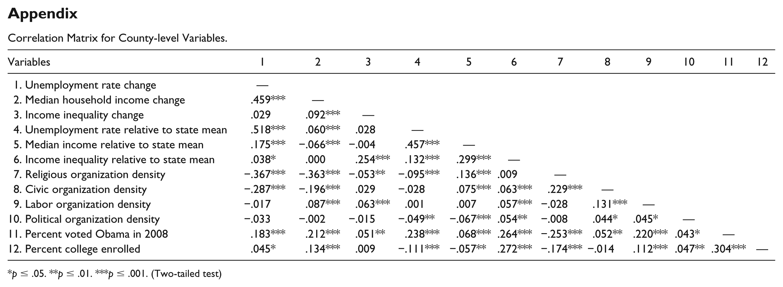
A few important notes are as follows: First, the ACS five-year Summary File data are multiyear estimates extending from January 1, 2005, through December 31, 2009, and from January 1, 2007, through December 31, 2011. Each measure, therefore, represents estimated values over the two five-year periods, which may moderate variability in the data. And, second, the correlations for each of the included predictors are low to moderate in strength (see the appendix). That is, there are no strong correlations between the primary independent variables of interest. Tests for multicollinearity between these variables all fall below the recommended variance inflation factor level of 2.5 (Allison 1999).

Modeling Technique

A generalized linear mixed model is used to evaluate the relative contributions of the predictors of economic threats and available resources. Regression analyses that utilize a mixed modeling technique are useful when data are nested in physical, social, and political contexts, such as counties within a state (Luke 2004). Mixed modeling corrects for potentially biased parameter estimates and standard errors that could result in an increased chance of Type I errors (Guo and Zhao 2000). The generalized linear mixed model follows the form:

\ln [p_{i j} / (1 - p_{i j})] = β_{0} + β_{k} x_{i j} + \dots + u_{j},

where p_ij is the probability of group formation within a given county; the intercept of β₀ is the expected value of the outcome when all predictors are held at zero, the slopes of the first-level predictors x_ij are β_k, and, finally, the error term is u_j, which is the unmodeled variance of the second level. The implicit assumption made by our random intercept mixed model is that different states had different average odds of the outcome given their unique contexts, but that the marginal effects of the county-level predictors were the same across states.

As can be seen in the map presented earlier in the paper (Figure 1), counties with Occupy groups may have significantly clustered within certain states due to their unique physical, social, or political characteristics. This is a preliminary indication that a mixed model may be a suitable modeling strategy to account for the previously unmodeled contextual effects. A further statistical test of a null specified model clustered by state reveals an intraclass correlation coefficient of .25, indicating that up to a quarter of the total differences observed in the county-level outcome are attributable to unobserved state-level factors. This statistical test affirms that a mixed model is a suitable strategy for pursuing the statistical analysis because significant variation exists between states, which could bias the results if left unaccounted.

In addition to accounting for these unobserved contextual factors, we employ a spatial adjustment parameter to “explain away” residual spatial dependence that might similarly bias our results. A simple method of incorporating the sum of the number of immediately adjacent county observations as a covariate in the model is used to alleviate the spatial diffusion observed in the dependent variable across the study area. This technique is comparable to a mixed regressive spatial autoregressive (MRSAR) model, where a lag of the dependent variable is used on the right-hand side of the regression equation alongside the other nonlagged predictor variables (Anselin 1988).¹²

Results

In the last four months of 2011, OWS mobilizations spread to some 625 counties, and county equivalents, across the continental United States. The map in Figure 1 above shows substantial spatial variation in the distribution of counties in which OWS groups formed. The effects of the Great Recession varied substantially across counties as well. As seen in Table 1 above, the intensity of disruptive and positional economic threats differed dramatically at the county level as did the amount of available resources. Clearly, the effects of the recession and its aftermath impacted counties quite differently with some undergoing severe economic threats as others prospered.

To illustrate this, consider the variation in disruptive economic threat between 2007 and 2011. Unemployment increased nationally by an average of 3.68 percent, yet across counties it ranged from a 13.3 percent increase to a decline of 3.3 percent. Over the same time period, overall median household incomes declined nationally more than $2,100, with the hardest hit county declining by more than $15,600. Yet, another county increased by more than $17,300. Similarly, overall income inequality within counties remained relatively unchanged between 2007 and 2011 (mean = .23), while some counties increased substantially (maximum = 11.23) as others declined (minimum = −14.97). Thus, declining economic conditions between 2007 and 2011 created more disruptive threats for some counties than others. Table 1 also shows substantial variation in positional economic threat across counties within states. In 2011, some counties fared much worse compared with other counties within their states, while others fared substantially better. For example, some counties had median household incomes roughly $28,600 less than the state average, whereas other counties had median household incomes exceeding $71,800 more than the state average. Social-organizational and human resource measures also show moderate to substantial local variation as do the control variables. In the analysis that follows, we examine how variation in economic threats and resource availability explain the pattern of OWS mobilization across American communities.

Multivariate Logistic Regression Analysis

Table 2 presents results for a series of logit regression models designed to assess support for the four hypotheses previously articulated. Coefficients reported are the odds ratios with the nonexponentiated coefficients and standard errors in parentheses. Odds ratios greater than 1.0 indicate a positive effect of the independent variable on the odds of an OWS mobilization and odds ratios less than 1.0 indicate a negative effect of the explanatory variable on the formation of an OWS SMO.

Table 2.

Odds Ratios from Mixed Model Logistic Regression of OWS Mobilization in U.S. Counties, 2011.

Variables	Model 1	Model 2	Model 3	Model 4
Disruptive economic threats (2007–2011)
Unemployment rate change	0.932	—	—	1.156
Unemployment rate change	(−0.071, 0.049)			(0.145, 0.102)
Median household income change^a	0.956	—	—	0.974
Median household income change^a	(−0.045, 0.024)			(−0.026, 0.028)
Income inequality change	0.970	—	—	0.952
Income inequality change	(−0.030, 0.053)			(−0.049, 0.058)
Positional economic threats (2011)
Unemployment rate relative to state mean	—	0.837***	—	0.831**
Unemployment rate relative to state mean		(−0.178, 0.037)		(−0.186, 0.053)
Median household income relative to state mean^a	—	1.042***	—	1.029**
Median household income relative to state mean^a		(0.041, 0.010)		(0.028, 0.010)
Income inequality relative to state mean	—	1.308***	—	1.185***
Income inequality relative to state mean		(0.268, 0.037)		(0.170, 0.039)
Social-organizational resources^b
Religious organization density	—	—	1.048	1.020
Religious organization density			(0.047, 0.031)	(0.020, 0.031)
Civic organization density	—	—	1.252**	1.211*
Civic organization density			(0.225, 0.094)	(0.191, 0.100)
Labor organization density	—	—	1.930***	1.831***
Labor organization density			(0.658, 0.240)	(0.605, 0.251)
Political organization density	—	—	2.138	2.114
Political organization density			(0.760, 0.982)	(0.749, 0.973)
Human resources
Percent voted Obama in 2008	—	—	1.020*	1.016
Percent voted Obama in 2008			(0.020, 0.009)	(0.016, 0.009)
Percent college enrolled	—	—	1.184***	1.128***
Percent college enrolled			(0.169, 0.021)	(0.121, 0.021)
Controls
Percent white	1.006	1.019**	1.017*	1.023**
Percent white	(0.006, 0.006)	(0.019, 0.007)	(0.017, 0.008)	(0.023, 0.008)
Population (ln)	3.781***	4.414***	3.607***	3.894***
Population (ln)	(1.330, 0.319)	(1.485, 0.442)	(1.283, 0.367)	(1.360, 0.445)
Population density^b	0.522*	0.288***	0.441**	0.317***
Population density^b	(−0.651, 0.134)	(−1.246, 0.075)	(−0.818, 0.111)	(−1.150, 0.083)
State capital^c	102.181***	174.704***	124.313*	123.372**
State capital^c	(4.627, 127.060)	(5.163, 216.888)	(4.823, 247.807)	(4.815, 227.765)
Spatial adjustment	2.035***	2.281***	2.274***	2.391***
Spatial adjustment	(0.710, 0.121)	(0.825, 0.149)	(0.822, 0.158)	(0.872, 0.174)
Intercept	3.17e−08***	9.48e−10***	5.25e−10***	1.68e−10***
Intercept	(−17.267, 3.82e−08)	(−20.777, 1.33e−09)	(−21.368, 9.15e−10)	(−22.510, 3.29e−10)
Variance component^d	.260***	.379***	.541***	.524***
Variance component^d	(.124)	(.168)	(.204)	(.210)
N ₁	3,106	3,106	3,106	3,106
N ₂	48	48	48	48
Log likelihood	−792.927	−706.273	−684.311	−656.132

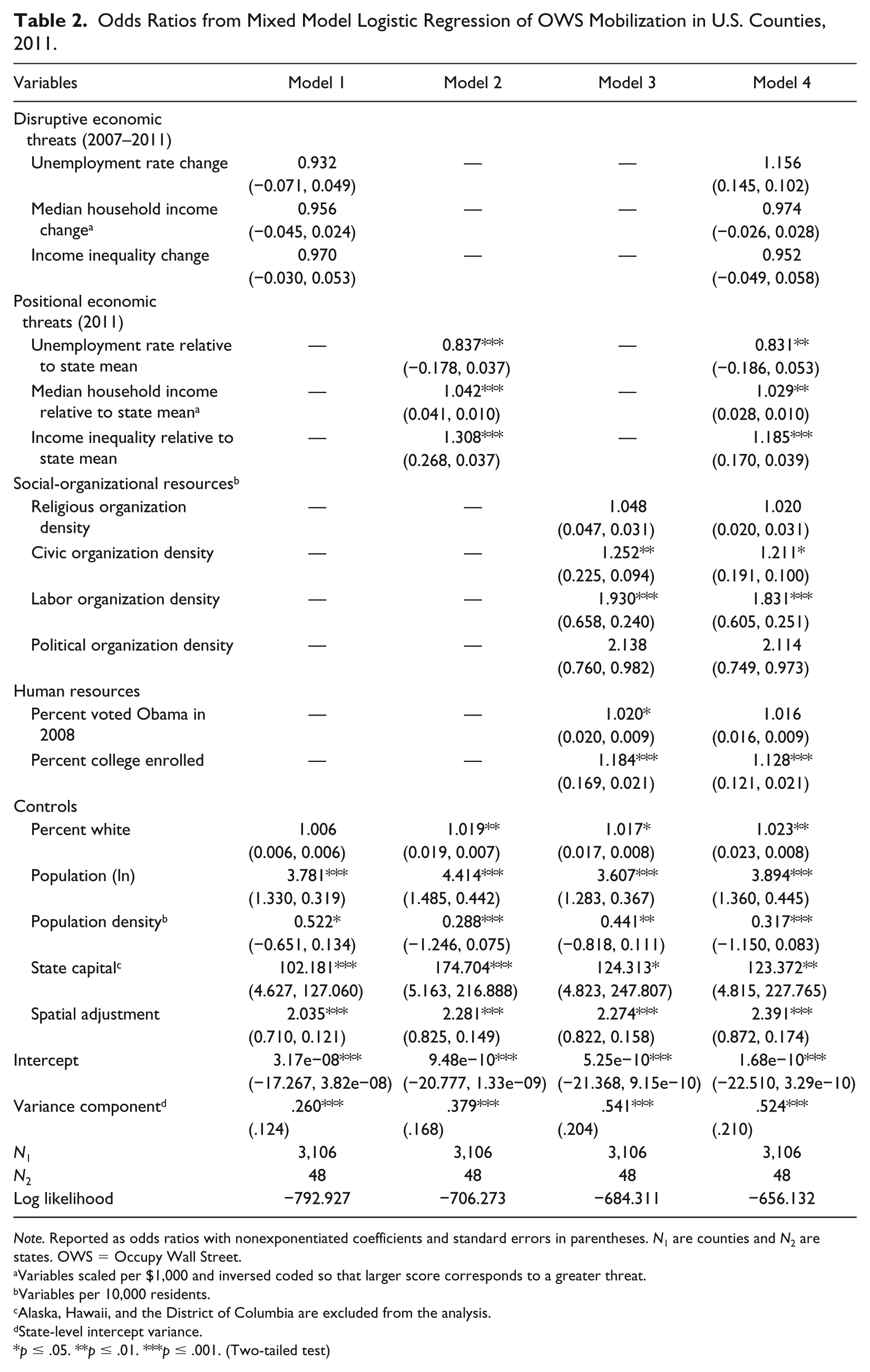
Note. Reported as odds ratios with nonexponentiated coefficients and standard errors in parentheses. N₁ are counties and N₂ are states. OWS = Occupy Wall Street.

Variables scaled per $1,000 and inversed coded so that larger score corresponds to a greater threat.

Variables per 10,000 residents.

Alaska, Hawaii, and the District of Columbia are excluded from the analysis.

State-level intercept variance.

p ≤ .05. **p ≤ .01. ***p ≤ .001. (Two-tailed test)

Models 1 to 3 present results of our theory derived analyses designed to test the possible effects of disruptive economic threats, positional economic threats, and preexisting social-organizational and human resources on movement mobilization while controlling for relevant county-level characteristics.

The results for Model 1 show no support for H1 that Occupy SMOs mobilized in reaction to disruptive changes in local economies. Results for Model 2 show greater, yet mixed support for H2 regarding the effect of greater positional economic threat within states on Occupy group formation. Counties with median household incomes that positioned them below their state average and income inequality that positioned them above their state average had greater odds of mobilizing OWS protest groups as indicated by odds ratios of 1.042 and 1.308, respectively. In contrast, counties with higher unemployment rates compared with their state average had lower odds of mobilization by a factor of .837. Results for Model 3 provide moderate support for H3 and H4 that the odds of Occupy group formation was higher in counties with greater social-organizational and human resources.

We now turn to Model 4, which includes all explanatory variables in a single saturated model, to get a fuller understanding of the relationships between economic threats and resource availability on local OWS protest mobilizations.

Disruptive economic threats

As with Model 1, the results in Model 4 provide no support for H1 on the impact of disruptive economic threats. That said, the coefficient for the disruptive economic threat of the change in the unemployment rate flips direction. However, this instability is likely not due to collinearity as tests for multicollinearity between the independent variables fall within generally accepted limits. Therefore, further statistical testing was employed which revealed a potential suppression effect whereby the directionality of disruptive unemployment changes only after positional unemployment is taken into account (see MacKinnon, Krull, and Lockwood 2000). Thus, among counties with comparable levels of positional unemployment in 2011, which overall exhibited a downward influence on the odds that an OWS group formed, those that had greater increases in unemployment rate between 2007 and 2011 may have exhibited greater odds of forming Occupy groups. But this inconsistent mediation effect does not reach statistical significance.

Positional economic threats

Model 4 provides mixed support for the impact of positional economic threats on localized protest mobilization. Consistent with H2, counties with the positional threats of lower household incomes and higher income inequality relative to state averages had increased odds of OWS protest group formation. Both of these effects are quite pronounced. For every additional $1,000 reduction in median household income compared with the state mean, positional household income increased the odds of OWS protest group formation by a factor of 1.029. To put this in a more meaningful context, given two otherwise identical counties, the one with an additional $1,000 reduction would have its odds of an OWS group being present increased by 2.9 percent. The effect of differences in positional income inequality also provide a substantial effect that is consistent with our second hypothesis. Each one-unit increase in the positional income inequality measure corresponds to an increased odds of OWS mobilization by a factor of 1.185. In other words, a county with a one-unit higher inequality score would have its odds of an OWS group being present increased by 18.5 percent compared with an otherwise equivalent county.

By contrast, counties with higher unemployment rates in 2011 compared with their state averages had lower odds of Occupy groups being present, contradicting H2. Thus, for each percentage point increase on the measure of positional unemployment, the odds of protest group formation decreased by a factor of .831. When interpreting odds ratios below 1.0, care needs to be taken as odds ratios are asymmetrical. Moreover, we are interested in understanding why groups formed in some locations, rather than why they did not form. Thus, we inverse the odds ratio to ease interpretation (Osborne 2015). The inversed odds ratio indicates that counties with lower unemployment rates relative to other counties in their state had higher odds that an Occupy group formed. A county with an unemployment rate 1.0 percent lower than the state average would have its odds that an OWS group mobilized increase by a factor of 1.203.

Social-organizational resources

Partial support for resource mobilization (H3) remains evident in Model 4 as OWS protest groups had increased odds to have mobilized in counties with a greater density of civic and labor organizations. For each additional civic organization per 10,000 residents in a county, the odds that an Occupy group mobilized there increased by a factor of 1.211. The result for labor organizations is even more pronounced. Compared with an otherwise equivalent county with zero labor organizations, a county with just one labor group per 10,000 residents had 1.831 times the odds of forming an OWS protest group, while a county with two labor organizations had more than twice the baseline odds.

Human resources

Model 4 provides positive but partial support for the effects of human resources (H4) on the formation of local OWS groups. Increases in the density of localized human resources, represented by an increased percentage of residents currently college enrolled, increased the odds of group formation, everything else being equal. This is also a substantial effect. For every percentage point increase in those currently college enrolled, the odds of OWS protest group formation increased by a factor of 1.128. Recall from Table 1 that the percentage of those enrolled in college ranged dramatically from zero percent to 52.01 percent among counties (with a standard deviation of 4.02 percent). The analysis here indicates that for a percentage point increase in the share of those in college, it raised the odds of OWS group formation by 12.8 percent. Thus, increased presence of college students strongly predicts the mobilization of Occupy groups. In contrast, the impact of county residents who had voted for Obama during the 2008, while statistically significant in Model 3, shows no effect in the saturated model.

Controls

Finally, we note that each control variable significantly predicts OWS protest group formation in Model 4. Occupy groups were more likely to form in counties with the state capital, larger populations but with lower population density (indicated by an odds score below 1.0), and higher proportions of residents self-identifying as white.

Discussion

During a three-month period in the fall of 2011, OWS protest groups emerged in about one in five American counties across the continental United States. What distinguished localities that mobilized from those that did not? The analysis here takes up that question and enhances theoretical understanding of local social movement mobilization in two ways. First, our analysis indicates that positional economic threats, rather than disruptive economic threats, affected local variations in the mobilization of OWS protests. Second, our analysis supports long-standing tenets of RMT that the localized mobilization capacity represented by preexisting reserves of human and social-organizational resources facilitate localized protest mobilizations. We discuss each of these theoretical contributions below.

Disruptive and Positional Economic Threats

Our results indicate the disruptive economic threats created by the Great Recession had no effect on the mobilization of OWS groups across counties, while positional economic threats had a significant though inconsistent effect. The noneffect of disruptive economic threats differs from earlier research (e.g., Juris 2012; Lubin 2012; McVeigh 2011) as well as media accounts (e.g., Kleinfield and Buckley 2011) claiming that OWS groups mobilized in reaction to the rapid and substantial deterioration of economic conditions caused by the Great Recession. The noneffect also counters previous research showing the importance of disruptive threats in other movement mobilizations (e.g., Bullard 2000; Walsh 1981). Positional threats mattered in that Occupy groups were more likely to form in counties where median household income lagged behind other counties in the state and where income inequality was more intense than in other counties.

Yet, contrary to our hypothesis about unemployment, relatively high unemployment reduced, rather than increased, the odds of localized mobilization. Why were counties that had relatively lower rates of unemployment more likely to have an OWS group form than localities with relatively higher rates of unemployment? In part, we speculate that residents living in places with low unemployment may have noticed their relatively better employment opportunities and also observed that the inequality and declining household incomes did not align with these labor market conditions. Thus, residents of relatively advantaged counties in terms of employment may have been more likely to mobilize because they assessed that locations with higher relative employment, like their own, ought to have relatively lower income inequality and higher household incomes but did not. This mismatch may have reinforced the collective view that economic advantages were not distributed equitably across their state. Moreover, whereas high unemployment may lead to the breakup of a local sense of community as people relocate to pursue gainful employment, just the prospect of job opportunities within the context of low unemployment may keep people integrated in their communities and involved in civic life.

Human and Social-organizational Resources

This research also shows the importance of resource distribution across locales in the mobilization of social movements as predicted by RMT. The positive impact of college enrollment in a county is consistent with the scholarly narrative that preexisting support networks of individuals and organizations facilitated the emergence of the initial Occupy mobilization in lower Manhattan (Milkman, Lewis, and Luce 2013; Piven 2013). The positive effect of a larger percentage of currently enrolled college students on the emergence of OWS protest in localities across the United States also supports previous research on the subject of student activism and suggests that college students constituted a mobilizable pool of individuals receptive to OWS messaging and recruitment efforts.

But, our other human resource, the presence of politically active residents who had voted for Obama in 2008, was not related to OWS mobilization. We speculate that the nonsignificance of Obama voters may be partially explained by the importance of social media in the formation of OWS groups as noted by Ion Bogdan Vasi and Chan S. Suh (2016) and Chan S. Suh, Ion Bogdan Vasi, and Paul Y. Chang (2017). Some Occupy groups were formed using social media platforms such as Meetup (the platform originally used to set up face-to-face meetings for people wanting to start an Occupy group in their location) and Facebook (a platform that was quickly adopted to disseminate information about Occupy groups that were forming and had formed). The salience of social media in the formation of Occupy groups suggests the human resource of people skilled at using social media platforms, such as students, was more important than previously politically active people, such as Obama voters. It is possible that online organizing efforts may have supplemented or substituted for the face-to-face organizing that Obama voters were hypothesized to provide but ultimately did not.

The preexisting social-organizational resources embedded in more extensive labor and civic infrastructures proved to be significant predictors of protest group formation. These results are consistent with resource mobilization scholarship which finds that emerging social movements often gain access to and utilize a range of resources embedded in preexisting local organizations (Edwards and McCarthy 2004). By contrast, our research shows that localized religious and political organizational infrastructures did not contribute to the formation of OWS groups as hypothesized. Given the clear left-of-center politics of OWS, it seems safe to assume that politically and socially conservative organizations would not have provided a strong resource base for localized OWS mobilizations.

Conclusion

The research presented here has sought to better understand the interplay of economic threats and mobilization capacity in the formation of OWS protest groups in local communities across the country. In general, our results support the continued integration of structural threats with indicators of local mobilization capacity drawn from RMT when investigating broad patterns of protest movement activity. Social movement scholars have already begun to reincorporate elements of economic hardship into theories of collective action (e.g., Caren et al. 2016; Grasso et al. 2017; Ward 2017), and the evidence presented here suggests the continuing merit of this approach for future research.

Our findings suggest three areas of future research. First, more work is needed to differentiate theoretically and empirically between disruptive and positional economic threats and understand why one type of threat better explains mobilization than another. When do disruptive economic threats impact movement mobilization compared with positional economic threats? Are there circumstances, or particular types of movements, where one type of economic threat matters most or where both types of economic threat interact? Second, future research needs to clarify whether disruptive and positional threats involve other aspects of social life besides economic concerns. For example, to what extent do disruptive and/or positional threats to public health caused by environmental pollutants contribute to the mobilization of protests? Finally, future research would do well to explore whether other types of threat related to countermovement dynamics may contribute to mobilization. For example, did the ideologically progressive Occupy movement mobilize—at least in part—as a response to the ideologically libertarian Tea Party movement, which had produced substantial political gains for conservatives in the 2010 mid-term elections? Such research could explain whether relevant ideological threats operate alongside economic threats to facilitate countermovement mobilizations.

Footnotes

Appendix

Correlation Matrix for County-level Variables.

Variables	1	2	3	4	5	6	7	8	9	10	11	12
1. Unemployment rate change	—
2. Median household income change	.459***	—
3. Income inequality change	.029	.092***	—
4. Unemployment rate relative to state mean	.518***	.060***	.028	—
5. Median income relative to state mean	.175***	−.066***	−.004	.457***	—
6. Income inequality relative to state mean	.038*	.000	.254***	.132***	.299***	—
7. Religious organization density	−.367***	−.363***	−.053**	−.095***	.136***	.009	—
8. Civic organization density	−.287***	−.196***	.029	−.028	.075***	.063***	.229***	—
9. Labor organization density	−.017	.087***	.063***	.001	.007	.057***	−.028	.131***	—
10. Political organization density	−.033	−.002	−.015	−.049**	−.067***	.054**	−.008	.044*	.045*	—
11. Percent voted Obama in 2008	.183***	.212***	.051**	.238***	.068***	.264***	−.253***	.052**	.220***	.043*	—
12. Percent college enrolled	.045*	.134***	.009	−.111***	−.057**	.272***	−.174***	−.014	.112***	.047**	.304***	—

p ≤ .05. **p ≤ .01. ***p ≤ .001. (Two-tailed test)

Acknowledgements

The first two authors made equal contributions to this work. The paper draws in part from master’s thesis. A preliminary version of this paper was presented at the 2016 Annual Meeting of the American Sociological Association in Seattle, Washington. The authors thank Courtney Mattoon for research assistance and Clark McPhail and anonymous reviewers for insightful comments on early drafts of the manuscript.

Declaration of Conflicting Interests

The author(s) declared no potential conflicts of interest with respect to the research, authorship, and/or publication of this article.

Funding

The author(s) received no financial support for the research, authorship, and/or publication of this article.

Notes

Author Biographies

Patrick F. Gillham, PhD, is an assistant professor of sociology at Western Washington University. His research examines social movement mobilization and demobilization, changes in the policing of protest and civil disorder, and innovations in protester strategies and tactics. His work has been published in Social Problems, Mobilization, Policing and Society, The Russell Sage Foundation Journal of the Social Sciences, International Sociology, and other scholarly outlets.

Nathan C. Lindstedt is a PhD candidate in Sociology at Washington State University. His research areas include social movements, environmental sociology, and quantitative methodology. His research interests include theories of action, discourse, consensus-making, decision-making, risk, and threat.

Bob Edwards is professor and Director of Undergraduate Programs in the Department of Sociology at East Carolina University. He has published over 50 chapters and articles on social movements, environmental sociology, social capital, and civil society. His work has appeared in the American Sociological Review, Annual Review of Sociology, Social Problems, Social Forces and a range of specialty journals.

Erik W. Johnson is an associate professor of sociology at Washington State University. His research examines the emergence, development and political outcomes of environmental movements. Ongoing research projects also examine changes over time in social correlates of environmental concern and development of the field of environmental crime.

References

Allison

Paul D.

1999. Multiple Regression: A Primer. Thousand Oaks, CA: Pine Forge Press.

Andrews

Kenneth

Biggs

Michael

. 2006. “The Dynamics of Protest Diffusion: Movement Organizations, Social Networks, and News Media in the 1960 Sit-ins.” American Sociological Review 71(5):752–77.

Anselin

Luc

. 1988. Spatial Econometrics: Methods and Models. Boston, MA: Kluwer Academic.

Armbruster-Sandoval

Ralph

. 2005. Globalization and Cross-border Labor Solidarity in the Americas: The anti-sweatshop Movement and the Struggle for Social Justice. New York: Routledge.

Bullard

Robert D.

2000. Dumping in Dixie: Race, Class, and Environmental Quality. 3rd ed. Boulder, CO: Westview Press.

Caren

Neal

Gaby

Sarah

Herrold

Catherine

. 2016. “Economic Breakdown and Collective Action.” Social Problems 64(1):133–55.

Christiano

Lawrence J.

2017. “The Great Recession: A Macroeconomic Earthquake.” Economic Policy Paper 17. Federal Reserve Bank of Minneapolis. Retrieved February 12, 2018 (https://www.minneapolisfed.org/~/media/files/pubs/eppapers/17-1/the-great-recession-a-macroeconomic-earthquake.pdf).

Chun

Yongwan

Griffith

Daniel A.

2013. Spatial Statistics and Geostatistics: Theory and Applications for Geographic Information Science and Technology. Thousand Oaks, CA: Sage Publications.

Crubaugh

Byant

. 2017. “Diversity, Poverty, and Resources: The Role of Incentives and Capacity in the Presence of Highly Resourced Neighborhood Associations.” Sociological Focus 50(2):138–58.

10.

Edwards

Bob

. 1995. “With Liberty and Environmental Justice for All: The Emergence and Challenge of Grassroots Environmentalism in the U.S.” Pp. 35–55 in Ecological Resistance Movements: The Global Emergence of Radical and Popular Environmentalism, edited by Taylor

New York: State University of New York Press.

11.

Edwards

Bob

Foley

Michael W.

2003. “Social Movement Organizations beyond the Beltway: Understanding the Diversity of One Social Movement Industry.” Mobilization: An International Quarterly 8(1):85–105.

12.

Edwards

Bob

Kane

Melinda

. 2014. “Resources and Social and Political Movements.” Pp. 205–32 in Handbook of Political Citizenship and Social Movements, edited by Van Der Heijen

Camberley, England: Edward Elgar.

13.

Edwards

Bob

McCarthy

John D.

2004. “Resources and Social Movement Mobilization.” Pp. 116–52 in Blackwell Companion to Social Movements, edited by Snow

Soule

Kriesi

London, England: Blackwell.

14.

Federal Reserve Economic Data. 2015. “The Evolution of Income Inequality.” The FRED Blog. Retrieved February 16, 2018 (https://fredblog.stlouisfed.org/2015/03/the-evolution-of-income-inequality/).

15.

Goldstone

Jack A.

Tilly

Charles

. 2001. “Threat (and Opportunity): Popular Action and State Response in the Dynamics of Contentious Action.” Pp. 179–94 in Silence and Voice in the Study of Contentious Politics, edited by Aminzade

R. R.

et al . New York: Cambridge University Press.

16.

Goodman

Christopher J.

Mance

Steven M.

2011. “Employment Loss and the 2007–09 Recession: An Overview.” Monthly Labor Review. Retrieved December 16, 2016 (https://www.bls.gov/mlr/2011/04/art1full.pdf).

17.

Gould-Wartofsky

Michael A.

2015. The Occupiers: The Making of the 99 Percent Movement. New York: Oxford University Press.

18.

Grasso

Maria T.

Yoxon

Barbara

Karampampas

Sotirios

Temple

Luke

. 2017. “Relative Deprivation and Inequalities in Social and Political Activism.” Acta Politica. 1–32. doi:10.1057/s41269-017-0072-y.

19.

Guo

Guang

Zhao

Hongxin

. 2000. “Multilevel Modeling for Binary Data.” Annual Review of Sociology 26:441–62.

20.

Inglehart

Ronald

. 1977. The Silent Revolution: Changing Values and Political Styles among Western Publics. Princeton, NJ: Princeton University Press.

21.

Jasso

Guillermina

. 2001. “Comparison Theory.” Pp. 669–98 in Handbook of Sociological Theory, edited by Turner

J. H.

New York: Kluwer Academic/Plenum Press.

22.

Jenkins

Craig J.

Perrow

Charles

. 1977. “Insurgency of the Powerless: Farm Worker Movements (1946–1972).” American Sociological Review 42:249–68.

23.

Juris

Jeffrey S.

2012. “Reflections on #Occupy Everywhere: Social Media, Public Space, and Emerging Logics of Aggregation.” American Ethnologist 39(2):259–79.

24.

Juris

Jeffrey S.

Ronayne

Michelle

Shokooh-Valle

Firuzeh

Wengronowitz

Robert

. 2012. “Negotiating Power and Difference within the 99%.” Social Movement Studies 11(3–4):434–40.

25.

Kahneman

Daniel

Tversky

Amos

. 1979. “Prospect Theory: An Analysis of Decision under Risk.” Econometrica 47:263–91.

26.

Kalleberg

Arne L.

Von Wachter

Till M.

2017. “The U.S. Labor Market during and after the Great Recession: Continuities and Transformations.” RSF: The Russell Sage Foundation Journal of the Social Sciences 3(3):1–19.

27.

Kim

Hyun Woo

McCarthy

John D.

2016. “Socially Organized Sentiments: Exploring the Link between Religious Density and Protest Mobilization, 1960-1995.” Social Science Research 60:199–211.

28.

Kleinfield

N. R.

Buckley

Cara

. 2011. “Wall Street Occupiers, Protesting Till Whenever.” The New York Times, October 1, pp. A1, A18.

29.

Liebig

Stefan

Sauer

Carsten

. 2016. “Sociology of Justice.” Pp. 37–59 in Handbook of Social Justice Theory and Research, edited by Sabbagh

Schmitt

New York: Springer.

30.

Lindstedt

Nathan

. 2015. “The Mobilizing Effect of Threat and Opportunity: A Mixed Model Analysis of the Occupy Movement.” MA thesis, Department of Sociology, Washington State University, Pullman, WA.

31.

Lobao

Linda M.

Hooks

Gregory

Tickamyer

Ann R.

eds. 2007. The Sociology of Spatial Inequality. Albany, NY: State University of New York Press.

32.

Lobao

Linda M.

Hooks

Gregory

Tickamyer

Ann R.

2008. “Poverty and Inequality across Space: Sociological Reflections on the Missing-middle Subnational Scale.” Cambridge Journal of Regions, Economy and Society 1:89–113.

33.

Lubin

Judy

. 2012. “The ‘Occupy’ Movement: Emerging Protest Forms and Contested Urban Spaces.” Berkeley Planning Journal 23:184–97.

34.

Luke

Douglas A.

2004. Multilevel Modeling. Thousand Oaks, CA: Sage Publications.

35.

MacKinnon

David P.

Krull

Jennifer L.

Lockwood

Chondra M.

2000. “Equivalence of the Mediation, Confounding and Suppression Effect.” Prevention Science: The Official Journal of the Society for Prevention Research 1(4):173.

36.

McAdam

Doug

. 1982. Political Process and the Development of Black Insurgency, 1930–1970. Chicago, IL: The University of Chicago Press.

37.

McAdam

Doug

. 1996. “Conceptual Origins, Current Problems, Future Directions.” Pp. 23–40 in Comparative Perspectives on Social Movements: Political Opportunities, Mobilizing Structures, and Cultural Framings, edited by Mcadam

Mccarthy

J. D.

Zald

M. N.

New York: Cambridge University Press.

38.

McAdam

Doug

McCarthy

John D.

Zald

Mayer N.

1988. “Social Movements.” Pp. 695–738 in Handbook of Sociology, edited by Smelser

N. J.

Newbury Park, CA: Sage.

39.

McAdam

Doug

Tarrow

Sydney G.

Tilly

Charles

. 1996. “Towards an Integrated Perspective on Social Movements and Revolution.” Pp. 142–73 in Comparative Politics: Rationality, Culture, and Structure, edited by Lichbach

M. I.

Kuckerman

A. S.

New York: Cambridge University Press.

40.

McCarthy

John D.

1996. “Mobilizing Structures: Constraints and Opportunities in Adopting, Adapting and Inventing.” Pp. 141–51 in Comparative Perspectives on Social Movements: Political Opportunities, Mobilizing Structures, and Cultural Framings, edited by Mcadam

Mccarthy

J. D.

Zald

M. N.

New York: Cambridge University Press.

41.

McCarthy

John D.

Wolfson

Mark

Baker

David P.

Mosakowski

Elaine

. 1988. “The Founding of Social Movement Organizations: Local Citizens’ Groups Opposing Drunken Driving.” Pp. 71–84 in Ecological Models of Organizations, edited by Carroll

G. R.

Cambridge, MA: Ballinger Press.

42.

McCarthy

John D.

Zald

Mayer N.

1977. “Resource Mobilization and Social Movements: A Partial Theory.” American Journal of Sociology 82(6):1212–41.

43.

McGurty

Eileen M.

2009. Transforming Environmentalism: Warren County, Pcb’s, and the Origins of Environmental Justice. New Brunswick, NJ: Rutgers University Press.

44.

McVeigh

Rory

. 2011. “How Occupy Wall Street Works: Why It Will Remain Nonviolent.” Foreign Affairs, October 10. Retrieved March 18, 2018 (https://www.foreignaffairs.com/articles/united-states/2011-10-10/how-occupy-wall-street-works).

45.

McVeigh

Rory

Beyerlein

Kraig

Vann

Burrel

Jr. Trivedi

Priyamvada

. 2014. “Educational Segregation, Tea Party Organizations, and Battles over Distributive Justice.” American Sociological Review 79(4):630–52.

46.

Meyer

David S.

Minkoff

Deborah C.

2004. “Conceptualizing Political Opportunity.” Social Forces 82(4):1457–92.

47.

Milkman

Ruth

Lewis

Penny

Luce

Stephanie

. 2013. “The Genie’s Out of the Bottle: Insiders’ Perspectives on Occupy Wall Street.” The Sociological Quarterly 54(2):194–98.

48.

Morris

Aldon

. 1984. The Origins of the Civil Rights Movement: Black Communities Organizing for Change. New York: Free Press.

49.

National Bureau of Economic Research. 2010. “Business Cycle Dating Committee, National Bureau of Economic Research.” Retrieved February 16, 2018 (http://www.nber.org/cycles/sept2010.html).

50.

Occupy Directory. 2011. “Occupy Directory.” Retrieved May 8, 2014 (http://directory.occupy.net/).

51.

Opp

Karl-Dieter

. 1988. “Grievances and Participation in Social Movements.” American Sociological Review 52(6):853–64.

52.

Osborne

Jason W.

2015. Best Practices in Logistic Regression. Thousand Oaks, CA: Sage Publications.

53.

Pettigrew

Thomas F.

1967. “Social Evaluation Theory: Convergences and Applications.” Pp. 241–311 in Nebraska Symposium on Motivation, edited by Levine

Lincoln, NE: University of Nebraska Press.

54.

Piven

Frances Fox

. 2013. “On the Organizational Question.” The Sociological Quarterly 54(2):191–93.

55.

Roper Center for Public Opinion Research. 2008. “How Groups Voted in 2008.” Retrieved February 18, 2018 (https://ropercenter.cornell.edu/polls/us-elections/how-groups-voted/how-groups-voted-2008/).

56.

Rosen

Ruth

. 2000. The World Split Open: How the Modern Women’s Movement Changed America. New York: Penguin Books.

57.

Rupasingha

Anil

Goetz

Stephan J.

2008. “US County-level Social Capital Data, 1990–2005.” University Park, PA: The Northeast Regional Center for Rural Development, Penn State University.

58.

Schneider

Nathan

. 2013. Thank You, Anarchy: Notes from the Occupy Apocalypse. Berkeley, CA: University of California Press.

59.

Smelser

Neil J.

1962. Theory of Collective Behavior. Glencoe, IL: Free Press.

60.

Snow

David A.

Cress

Daniel M.

Downey

Liam

Jones

Andrew W.

1998. “Disrupting the ‘Quotidian’: Reconceptualizing the Relationship between Breakdown and the Emergence of Collective Action.” Mobilization 3(1):1–22.

61.

Suh

Chan S.

Vasi

Ion Bogdan

Chang

Paul Y.

2017. “How Social Media Matter: Repression and the Diffusion of the Occupy Wall Street Movement.” Social Science Research 65:282–93.

62.

Tilly

Charles

. 1978. From Mobilization to Revolution. New York: Random House.

63.

Turner

Ralph H.

Killian

Lewis M.

1972. Collective Behavior. Englewood Cliffs, NJ: Prentice Hall.

64.

U.S. Census Bureau. 2007. “Small Area Income and Poverty Estimates, State and County Estimates for 2007.” Retrieved May 8, 2014 (https://www.census.gov/data/datasets/2007/demo/saipe/2007-state-and-county.html).

65.

U.S. Census Bureau. 2010. “2010 Census Gazetteer Files.” Retrieved March 1, 2018 (https://www.census.gov/geo/maps-data/data/gazetteer2010.html).

66.

U.S. Census Bureau. 2011a. “Small Area Income and Poverty Estimates, State and County Estimates for 2011.” Retrieved May 8, 2014 (https://www.census.gov/data/datasets/2011/demo/saipe/2011-state-and-county.html).

67.

U.S. Census Bureau. 2011b. “2005–2009 American Community Survey.” Retrieved May 8, 2014 (https://www2.census.gov/acs2005_2009_5yr/summaryfile/).

68.

U.S. Census Bureau. 2011c. “2007–2011 American Community Survey.” Retrieved May 8, 2014 (http://www2.census.gov/acs2011_5yr/summaryfile/).

69.

U.S. Department of Agriculture. 2014. “County-level Data Sets.” Retrieved May 8, 2014 (http://www.ers.usda.gov/data-products/county-level-data-sets/).

70.

U.S. Department of Labor. 2016. “Labor Force Statistics from the Current Population Survey.” Bureau of Labor Statistics. Retrieved December 20, 2016 (https://data.bls.gov/timeseries/LNS14000000).

71.

U.S. Geological Survey. 2009. “2008 Presidential General Election, County Results.” Retrieved May 8, 2014 (https://www.sciencebase.gov/catalog/item/4f4e49e6e4b07f02db5e71c6).

72.

van Dyke

Nella

. 2003. “Crossing Movement Boundaries: Factors That Facilitate Coalition Protest by American College Students, 1930–1990.” Social Problems 50(2):226–50.

73.

van Dyke

Nella

Soule

Sarah A.

2002. “Structural Social Change and the Mobilizing Effect of Threat: Explaining Levels of Patriot and Militia Organizing in the United States.” Social Problems 49(4):497–520.

74.

Vasi

Ion Bogdan

Suh

Chan S.

2016. “Online Activities, Spatial Proximity, and the Diffusion of the Occupy Wall Street Movement in the United States.” Mobilization 21(2):139–54.

75.

Walsh

Edward

. 1981. “Resource Mobilization and Citizen Protest in Communities around Three Mile Island.” Social Problems 29(1):1–21.

76.

Ward

Matthew

. 2017. “Opportunity, Resources, and Threat: Explaining Local Nativist Organizing in the United States.” Sociological Perspectives 60(3):459–78.