



Abstract
Developmental criminology suggests that the elements of one’s criminal career (such as specialization or frequency) are best captured through an understanding of their dynamic properties. To that end, this article introduces the Life History Plot: a graphic approach to understanding the important events that take place in an individual’s criminal and personal history. Each plot provides a visualization of the individual’s criminal history as well as marriage, children, employment, military service, time in custody, foster care, psychiatric history, and serious accidents. Life History Plots were created for a selection of chronic sexual offenders drawn from the Massachusetts Treatment Center Database. This article details the methods used to create the plots and encourages further exploration of data visualization techniques in criminology. Life History Plots make an important contribution to the field by allowing multiple aspects of an individual’s life to be instantly observed in a single graphic. This is a valuable tool that provides a visual summary of an individual’s life. Its utility for both research and clinical work is discussed.
The criminal career paradigm provides a framework in which to explore patterns of offending over time including onset, frequency, escalation, specialization, and desistance (Piquero, Farrington, & Blumstein, 2007). An appreciation of these components takes us beyond the view of crime as a static phenomenon and perhaps beyond the alleged distinction between criminals and noncriminals. Instead, it acknowledges that engaging in criminal behavior is a fluid process that ebbs and flows over time.
Many of the available approaches that measure the individual elements of the criminal career (e.g., including frequency, specialization, or versatility) tend to operate as if they are static and thus do not account for changes over time. Consistent with this perspective, some researchers have argued that these components might be best understood through a more comprehensive examination of the local life circumstances that an individual experiences across their life course (Sullivan, McGloin, Pratt, & Piquero, 2006). Growing interest in the timing and sequencing of important life events has led to the development of a number of different approaches to understanding this material temporally (Axinn, Pearce, & Ghimire, 1999). Because the nature of one’s offending changes over time (Wikstrom, 1987), it is important to explore specialization, escalation, and other offending tendencies as dynamic properties (LeBlanc & Frechette, 1989). Thus, the first rationale for this work is motivated by the need to attend to these shortcomings by creating a method that views these elements of the criminal career across the life span.
Although the criminal career paradigm is a standard observation in understanding general crime, it has been considered to a lesser extent for sexual offending (Hanson, 2002; Lussier, Proulx, & LeBlanc, 2005; Smallbone & Wortley, 2004). Previous studies have explored age of onset (Prentky & Knight, 1993), specialization (Harris, Mazerolle, & Knight, 2009a; Harris, Smallbone, Dennison, & Knight, 2009b), and escalation (Stermac & Hall, 1989), for example. Some studies find similarities between sexual offenders and generic offenders (Lussier et al., 2005; Simon, 2000) and others maintain that the samples differ importantly from one another (Laws & Marshall, 1990). Developmental and life course criminology likely provides a relevant theoretical lens through which to view sexual offending, but no one has yet satisfactorily applied this perspective to sexual offending over time. The second rationale for this work then is to contribute to what is known regarding the temporal nature of sexual offending and the extent to which it changes over time, on an individual level.
Although the quantitative exploration of event histories has piqued the interest of some researchers, there has been comparatively little progress in the actual development of information graphics and data visualization in developmental and life course criminology (Francis & Pritchard, 1998). This is likely due to the overwhelming complexity of many criminological datasets and the substantial time and cost that is involved in the creation of any kind of graphic. Data visualization represents somewhat of a departure for criminology, where there is a traditionally heavy reliance on cross-sectional sampling methods and spreadsheet-based statistics. These data do not easily lend themselves to longitudinal analysis or to answering qualitative questions. Therefore, the third rationale of the present study stems from Maltz’s (1998) call to action on the specific topic of data visualization in criminology. In a way, this article is a response to his appeal for the field to consider the benefits of representing criminological elements in graphical ways. Finally, as images now play an increasingly important role in our lives and as the technological capabilities of advanced software become more widely available, the previous obstacles of time and cost can more easily be overcome (Wheeldon & Ahlberg, 2012).
The present study introduces the Life History Plot: a graphic approach to understanding the important events that take place in an individual’s criminal and personal history. Although the plots may be created for any offender, or, in fact, any individual, the present demonstration explores a sample of sexual offenders. The advantages of this method (as it relates to the present sample) are 3-fold. First, it contributes to the little that is known about sexual offending patterns from the perspective of criminal career research. Second, it provides a vehicle by which the offending tendencies of a group of chronic sexual offenders are able to be explored in depth. Third, it achieves these two objectives visually, and generates an individual-level graphic representation of the criminal career. Finally, although not an initial objective of the work, the clinical utility of these plots from a therapeutic standpoint has been an exciting “side product.”
A Dynamic View of Criminal Careers
Previous studies of specialization have typically treated this offending tendency as a static measure. The two most commonly used measures of specialization, the specialization threshold (Harris, 2008; Harris et al., 2009b; Miethe, Olson, & Mitchell, 2006) and the diversity index (Harris, 2008; Harris et al., 2009b; Mazerolle, Brame, Paternoster, Piquero, & Dean, 2000), for example, provide an estimation of the proportion of an individual’s charges or convictions that are concentrated in a specific area (like property crime or violent crime). These techniques classify offenders based on their total offending history. For example, if more than 50% of an individual’s total number of charges is for a sexual offense, that offender would be considered a specialist sexual offender (Harris et al., 2009a, 2009b). Evidently, these methods do not account for the length of time between offenses, or the sequencing of individual charges.
More consistent with criminal career research, specialization might instead be better understood through an individualized measure of offending patterns (Sullivan et al., 2006; Williams & Arnold, 2002). Wikstrom (1987), for example, concluded that “different periods of life are criminogenic in different ways” (p. 200) and suggested that the nature of one’s offending likely changes over time. Similarly, LeBlanc and Frechette (1989) recommended that specialization be explored as a dynamic property within the context of desistance. They define specialization as “the concentration of criminal activity, which has previously been expressed in a variety of forms, into a limited number of crime categories” (LeBlanc & Frechette, 1989, p. 129).
These researchers argued that specialization be detected over time and would appear whenever an individual comes to focus more on a certain crime or crime category to the exclusion of others (LeBlanc & Frechette, 1989). By way of example, consider an offender with five offenses (theft, drugs, assault, vandalism, and unlawful use of a motor vehicle) committed in adolescence. Then at the age of 30, he commits acts of child molestation exclusively. LeBlanc and Frechette (1989) rightly point out that his criminal career is meaningfully different from someone who has accrued the same number and type of offenses randomly over the same period of time. A single aggregate measure of offense specialization (like the ones described previously) will evidently fail to distinguish between two individuals such as these.
To attend to these criticisms, some studies have defined specialization in a way that accounts for transitions over time. Measures such as the forward specialization coefficient (Farrington, Snyder, & Finnegan, 1988; Paternoster, Brame, Piquero, Mazerolle, & Dean, 1998; Miethe et al., 2006) use Markov chain analysis to create transition matrices that examine the nature of an offense, given the nature of the one that occurred immediately prior to it (Farrington et al., 1988; Paternoster et al., 1998). Although these methods capture the temporal nature of offending, they fail to account for between-individual differences.
The present study proposes that a dynamic account of offense specialization across a specific criminal career could be best articulated by plotting an individual’s charges in each crime category arranged by seriousness, and, over time, in a timeline-type chart. This approach provides a graphic representation of an individual’s criminal and personal history. This method also attends to the shortcomings of the other approaches by allowing for detection of escalation, desistance, and crime switching over time. Its descriptive contribution, in concert with other approaches, provides a more complete picture of offense specialization and versatility on an individual level.
Data Visualization in Criminology
Maltz (2010) strongly promotes the visualization of data as a first step in statistical analysis. Rather than seeing this as “data snooping,” he argues that it is actually good practice to begin any analysis by looking for potential patterns or relationships in the data. An advantage of this method is the detection of outliers that might be due to human error during data entry or indicative of exceptional cases that warrant further examination (Francis & Pritchard, 1998; Maltz, 2010). An additional advantage of “picturing” the data as an initial step is the identification of patterns that might characterize groups of individuals and the possibility of generating hypotheses that might inform subsequent analysis (Maltz, 1998).
Just like the range of sophisticated statistical techniques that are available, there is no one standard means of visualizing data. Such examples might include anything from basic pie or bar charts, to trellis plots, or network graphs. It is preferable, however, to try different techniques on specific data to determine which approach makes the most sense for that particular type of information (Maltz, 2010). As Maltz (2010) argues, “plotting data in different ways permits the analyst to obtain information from the dataset that would normally not be possible using standard (nonvisual) social science methods” (p. 28). He has also argued that complex patterns might end up being concealed simply as a consequence of the very analytical tools and processes that criminologists typically use (Maltz & Mullany, 2000).
Along these lines, Wild (in Maltz, 1998) predicted more than a decade ago that “the primary language for promoting the human understanding of data will be sophisticated computer graphics rather than mathematics” (p. 398). Although data visualization has thrived in many areas of social inquiry, criminology has been comparatively slow to adopt these techniques. With its focus on the understanding of social factors through cross-sectional analysis of large samples, relatively little attention has been paid to examining individual differences.
Nevertheless, various attempts have been made to visualize criminological research questions. These have included event charts, lexis pencil diagrams, and timelines. Event charts (Golman in Maltz & Mullany, 2000) have mostly been used to display medical survival data but have the potential to also illustrate recidivism. Lexis pencil diagrams (Francis & Pritchard, 1998) represent various dimensions of an event history graphically, using three-dimensional pencil shaped icons where each facet of the pencil is a different life domain (e.g., marriage, education, and employment). Graphic timelines. use a confusing selection of icons and colors to portray various life course data across different domains of activity (such as education, children, relationships, employment, substance abuse, and crime; Klosak in Maltz & Mullany, 2000).
In recent years, there have been some advances in visualizing social science research including geographical information systems (GIS) analysis (Batsche & Reader, 2012), crime mapping, spatial analysis (Youstin, Nobles, Ward, & Cook, 2011) and genograms (Weiss, Coll, Gerbauer, Smiley, & Carillo, 2010). GIS is a computer system that captures and organizes information within the context of geography. Although originally developed to examine land use, it has since been applied to the study of various “human behaviors that can be measured by or influenced by distance” (Batsche & Reader, 2012, p. 26). Recently, GIS technology has been used for an array of purposes such as in the study of spatiotemporal patterns of terrorist incidents (e.g., Medina, Siebeneck, & Hepner, 2011), the identification of affordable housing and proximity to certain social services, and understanding the individual process of transitions from foster care (Batsche & Reader, 2012).
Crime mapping or geocoding assesses the spatial association between pairs of events or incidents. This technique was recently employed in a study of the “near repeat” phenomenon, testing whether certain areas that have experienced a particular crime are at a greater risk of experiencing repeat victimization (Youstin, et al., 2011).
The genogram is a third example of the use of data visualization in social sciences. Most often used in counselor and therapist training, the genogram is a graphic representation of the nature of relationships across generations in a person’s family (Lim, 2008; Weiss, et al., 2010). By drawing different kinds of lines between individuals, it is possible to examine the nature of family dynamics. The genogram or “family mapping diagram” is typically used by clinicians as a data gathering tool for assessment but also in the context of therapeutic intervention.
Of all of the criminological questions, the examination of life histories seems especially appropriate for data visualization. Developmental and life course criminology acknowledge that even “if people experience similar events, they may have entirely different reactions to them” (Maltz & Mullany, 2000, p. 255). For example, the death of a parent might devastate one person, but free another from a lifetime of abuse. Whether one subscribes to Gottfredson and Hirschi’s (1990) argument that a person’s propensity for criminality is stable across their life; to Sampson and Laub’s (1993) perspective that early childhood experiences can be negated by subsequent, later experiences; or to Moffitt’s (1993) combination approach that some individuals can change their behaviors, but not as easily as others (Maltz & Mullany, 2000), it is necessary to examine events across the life course on an individual level.
Developmental perspectives tend to favor individual-level explanations over variable-level explanations. When the unit of analysis is a person, however (as is the case for life histories) it becomes possible to focus on how events are sequenced over time, how those events interact with each other, and how the individual is affected by those variables (Maltz & Mullany, 2000). The Life History Plot provides a method by which various important events in one’s life can be represented visually. Each important event can be observed in context and compared to other events that may have preceded, followed, or co-occurred with it.
Maltz and Mullany (2000) establish three further advantages of plotting the timing of events that are experienced by an individual. First, events are differentially meaningful across time. For example, the impact of sexual abuse will be different for a child of 5, compared to a child of 16, or for an adult. Second, it is necessary to consider life events in a historical context, where unemployment or divorce might be experienced differently during a time of war, or an economic recession, for example. Third, cohort effects are similarly important. Military service during the conflicts in Vietnam or Korea (as was common for the participants in the present sample) might be especially distinct from military involvement during a time of peace (Maltz & Mullany, 2000).
Method
Participants and Data Source
Participants were selected from a larger sample of over 800 men convicted of sexual offenses and referred for civil commitment at the Massachusetts Treatment Center (MTC) in Bridgewater, Massachusetts, between 1959 and 1991. The MTC was established in 1959 under special legislation (General Law of Massachusetts, ch. 123A Supp 1948; 1965 para 1–11) for the purpose of assessing and treating individuals convicted of repetitive and/or aggressive sexual offenses (Lieb, Quinsey, & Berliner, 1998). The present study drew largely from data that were previously coded from the information contained within participants’ archival files (Harris, 2008; Knight & Thornton, 2007).
The objective was to examine the offending and life circumstances of an especially chronic sample of men convicted of serious sexual offenses. Participants were sorted by length of criminal career and total number of charges. The most chronic participants were then selected based on the following characteristics: (1) their rap sheets contained at least 20 separate, officially recorded charges and (2) the time between their first recorded offense and their index offense exceeded 20 years. There were 32 participants who shared these characteristics. Although Life History Plots were generated for each of them, due to space constraints, the four most exemplary cases that best demonstrated the similarities and differences across cases were chosen to include in this article.
Some general descriptive statistics regarding the 32 chronic offenders that were originally selected for the study are contained in Table 1. The majority of the sample was White (87.5%) and Catholic (62.5%). Almost three quarters (71.9%) of the men were classified as extrafamilial child molesters and less than 10% were classified as rapists. A further 12.5% had both adult and child victims and the remaining 3.1% committed incest exclusively. Almost two thirds of the sample were evaluated to be “sexually dangerous persons” and committed for treatment (62.5%) and the remaining third were observed, determined not to be sexually dangerous and subsequently released. The average age of official criminal onset among the chronic offenders was 15.18 years and they were approximately 30.11 years old at the time of their index offense. On average, they accrued 37.9 charges over a period of 24.57 years.
Descriptive Analysis of Chronic Offenders (n = 32).

Note. IQ, intelligence quotient.
The MTC database is to sexual offending research what the Glueck Men (Glueck & Glueck, 1930, 1950) are to criminology. Also, given the historical nature of the present sample, it is interesting to note that many of the men in the sample (who were referred to the MTC as adults, mostly during the 1960s or 1970s) were also admitted to reformatories and training schools in the Boston area as children (during the 1930s and 1940s). In many cases, they spent time at the Lyman School for Boys and the Shirley Industrial School for Boys, specifically. A deeper exploration of the individual characteristics of the men in the sample revealed that approximately 90% of them were White, and many grew up in working class families, living in overcrowded homes in low socioeconomic areas of Boston. This has led the author to conclude that many of the men in the sample (approximately 125) might also have been included in Glueck and Glueck’s (1930, 1950) landmark study of delinquency as well as in Sampson and Laub’s (1993, 2003) subsequent studies of crime and desistance across the life course. Further, many of the participants (n = 84) who were referred to the MTC as adults and who were born in the “Glueck window” (1924–1932) did not serve time as juveniles and may be members of the 500 nondelinquent sample. Evidently, these men would likely constitute the sample that was not subsequently followed up by Laub and Sampson (2003). Given the size of Glueck and Glueck’s (1930) original delinquent sample (500) and the capacity of the Lyman School (250–300 13- to 15-year-old boys) and the Shirley School (150–200 15- to 17-year-old boys) at the time (Miller, 1998), it seems a realistic possibility that the samples overlap.
Procedure
The first step in the construction of the Life History Plot was to complete a Life History Calendar (Laub & Sampson, 2003) for each participant. Life History Calendars allow for the time (year), length, and frequency of major life events to be plotted by age. These life events usually include arrests, convictions, residences, housemates, family, marriage, children, employment, military, and custody. Laws and Ward (2011) explain that these calendars can be partially completed from official records, but ultimately require the offender’s self-report, and if possible, the ability to crosscheck details from more than one source.
Although the present study is limited by the use of archival data exclusively, it should be noted that these data come from extensive clinical files which include court reports, criminal records, police reports, school and employment records, correspondence sent and received during treatment, psychological reports, clinical assessments, and interviewer notes.
All relevant details were extracted from previously coded, secondary data in the MTC database (which is maintained using SPSS) and entered into electronic life history calendar spreadsheets in Microsoft Excel. Next, with the assistance of a graphic designer and programmer (D. Harris, personal communication, December 10, 2010), criminal records and pertinent life history events were plotted using code in Processing, a free and open-source language designed at Massachusetts Institute of Technology to make visual display of information easy (Reas & Fry, 2007).
The original list of variables included births and deaths of parents, siblings, and children; substance abuse histories; educational disruptions; parental separation; and number of residences. As the life history plots began to be built, however, it became abundantly clear that there was a limit to how many items could be displayed meaningfully (and usefully) on a single plot and in some cases (regarding child abuse, specifically) the files did not provide sufficient information. Thus, the final list of variables included official criminal record (year and type of individual charge [miscellaneous, property, nonsexual violent, sexual]) and timing and length of foster care, incarceration, employment, military involvement, and marriages (or marital type relationships). These variables were ultimately selected for their relevance to sexual offending and because they were reported consistently across cases. In addition to these components, the graph plots number of children (and their year of birth); year of first sexual experience (including age and gender of partner); years and frequency of serious physical trauma (such as accidents, fights, or suicide attempts), in-patient psychiatric evaluations, and self-reported substance abuse. It should be acknowledged that although this list of variables was appropriate for the present sample, it is likely that different variables might emerge as especially relevant for other more contemporary samples, or for different types of offenders. Because the plots are automated, other variables can be substituted into future versions as appropriate. A description of this and other options are provided in further detail in the discussion.
Results
Of the 32 cases that were initially plotted, 4 are presented in this article. 1 These four cases were chosen for their ability to demonstrate the utility of the Life History Plot. They each share similar characteristics (including number of charges, age of official criminal onset, and criminal career length), but also have unique histories (including military involvement, marriage, parenthood, and foster care). A brief description of each case is contained here, but readers are encouraged to view the plots first to familiarize themselves with their format.
The central timeline indicates how time is spent. Shading along this line illustrates whether the individual was in foster care (orange shading), in custody (black shading), in the military (brown shading), or gainfully employed (purple shading). The units of analysis along this line are years and they are marked at 10-year divisions. Time when the line is not shaded (white) indicates unemployed, nonoffending street time.
The icons under the central timeline specify important events including (in ascending order from the bottom of the plot) first sexual experience (with age and gender of partner noted); in-patient psychiatric evaluations; and, serious accidents or trauma (such as head injuries/concussions or broken bones). Marriages are shown just below the central timeline by a rectangular box (indicating the length of the relationship) and a line and boxes stemming from it indicate children born of that marriage. The official criminal record is featured above the central timeline.
Each stem represents 1 year and each circle on a stem indicates an officially recorded offense. The height of the circle indicates the seriousness of the offense and the area of the circle is proportional to the number of charges for that offense in that year. (So, a large circle could indicate either multiple charges for the same offense, brought against a person on one occasion or repeated charges that might have occurred weeks or months apart for the same crime type, in that year.) Crimes are arranged into four offense categories (in order of increasing seriousness): miscellaneous, property, nonsexual violence, and sexual offenses. Within those categories, there are 19 levels (Harris, 2008). In ascending order, from the central timeline, “Miscellaneous” includes motor vehicle offenses and traffic violations; justice-related and military offenses; public order offenses; alcohol-related offenses; and drug-related offenses. “Property” includes general property offenses; weapons; white-collar crime; theft and larceny; and burglary or breaking and entering. “Violence” includes robbery; abduction and kidnapping; dangerous or negligent acts that cause bodily harm (including driving under the influence of alcohol or drugs); and assault. “Sexual offenses” include noncontact sexual offenses against adults or children (including indecent exposure or voyeurism), child molestation, rape, and sexual assault. Attempted or completed homicide is indicated by a circle above all of the other categories.
Figure 1 contains the Life History Plot of Case A. Case A was born in 1931 and was referred for civil commitment while serving a custodial sentence for two incidents of sexual assault that occurred when he was 36 years old. At the time that the data were collected, he was still in custody, at the age of 42. The Life History Plot shows that he lived in foster care for 5 years, from ages 10 to 15. His age of onset was 15. His first officially recorded offense included several property crimes for which he served a year in juvenile detention. His first sexual experience occurred the same year, with a 26-year-old woman. He reoffended at 19 with another property offense and again received a custodial sentence. He spent much of the next 20 years in custody and was apparently only on the street long enough to reoffend and be reincarcerated. His criminal career was marked by a versatile array of property, miscellaneous, and violent offenses, including acts of violence and property damage that he committed while in custody. At a glance, it is possible to detect some escalation in offending, where he appears to have progressed from property, to violence, to sexually violent offending. He was married for a few years in his mid-20s and had two children. His sexual offenses did not start until his mid-30s and do not appear to have followed any specific pattern. They are likely representative of his involvement in general criminal behavior.

Life history plot Case A. (See online for color publication. In the print version, these colors are rendered as shades of grey).
The Life History Plot of Case B is featured in Figure 2. It is immediately clear that although they were approximately the same age at referral to the MTC, and had amassed a similar number of charges over their criminal career, Case B and Case A are considerably different. Case B’s archival records did not include any specific information about his first sexual experience, and it appears that he lived with his family of origin until serving 4 years in the military. His age of onset was relatively late, at 24 years of age, and began with sexual violence. Although charged, he did not serve any time for this offense (and might not have been convicted). Case B had two marriages. He met his first wife while serving in the military and the relationship lasted 6 years. His second marriage began shortly after his first divorce and resulted in four children. Although he worked for a few years after leaving the army, he has not worked since. His index offense involved more than 30 separate incidents of child molestation and child pornography–related offenses (brought against him at a single court appearance) as well as numerous “miscellaneous” charges including contributing to the delinquency of a minor.

Life history plot Case B. (See online for color publication. In the print version, these colors are rendered as shades of grey).
Case B is a specialized, persistent, sexual offender. This plot appears to suggest that all of the incidents of child molestation occurred in the same year. Although this is consistent with the official rap sheet, it is probable that the sexual offending actually occurred over a longer period of time. That is, the fact that the charges were brought against him on a single day does not represent the true temporal ordering of that offending. Gathering this type of information from an interview or a survey, for example, would be a useful way of assessing the specific dates. This type of data collection is recommended for future assessments, and discussed in more detail below.
A simple glance at the Life History Plot of Case C (Figure 3) suggests a high functioning, gainfully employed, married father of seven whose criminal career is almost exclusively sexual. He was born in 1928 and his first sexual experience occurred with an 11-year-old girl when he was 16. That same year he committed his first offense (which was sexual in nature) and received a custodial sentence. After his release from detention, he worked for approximately 5 years before reoffending with two sexual offenses and one violent offense and serving 3 years in custody. He married when he was 27, and his wife had 7 children. He worked steadily for 10 years—from the birth of his third child until just before he was incarcerated for his index offense. His index offense involved more than 30 separate counts of incest over a period of 3 years. This is shown by three circles (each representing 10 charges) on three stems (each representing 1 year). The interview notes, police reports, and court transcripts in the archival records indicate that Case C victimized his two eldest daughters (the children denoted with a “v”) weekly over a period of 3 years. His marriage ended when he went to prison for these offenses. Although the official record (as represented in the plot) grossly underestimates the actual amount of offenses likely committed by Case C (as detailed in the file), it can still be considered a reasonable indicator of his criminal career, relative to other participants.

Life history plot Case C. (See online for color publication. In the print version, these colors are rendered as shades of grey).
The Life History Plot of Case D is featured in Figure 4. Case D was born in 1945 and committed his first offense (robbery) at the age of 9. While living with his birth parents, he was knocked unconscious and had multiple head injuries during his childhood and adolescence. He was a persistent, versatile offender who committed property offenses, multiple acts of violence, and miscellaneous crimes. His first sexual experience occurred with a 13-year-old boy, when he was 13. In the interview transcripts detailed in his file, he admitted to committing numerous thefts in his teenage years for which he was never caught (these events are not included in the plot). His first sexual offense occurred at age 18 and he received a custodial sentence. He committed his index offense at age 34. He was incarcerated for much of his adolescence and adulthood and received his first custodial sentence at the age of 12. He was held in juvenile detention on five separate occasions for violent and property offenses. During his longest stay in custody, he committed multiple property offenses and attacked a guard on two separate occasions. He was never married, never had children, never held a job, and never served in the military. He received an in-patient psychiatric evaluation at least 15 times between his 19th and 34th birthdays, sometimes up to 3 times in 1 year.
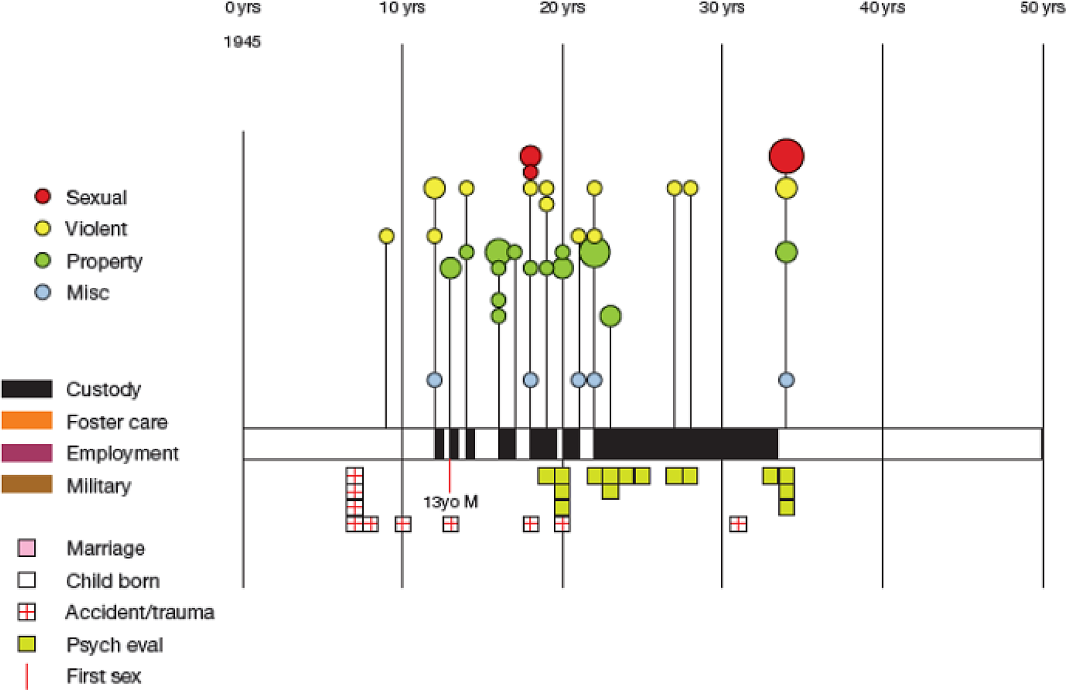
Life history plot Case D. (See online for color publication. In the print version, these colors are rendered as shades of grey).
Discussion
The Life History Plot is a graphic timeline-based chart that provides an individualized examination of a criminal career. Each plot shows the date (year) and type of various life events (such as marriage, family, and employment histories) while preserving their chronological sequencing. It also contains the sequence of offenses committed throughout their criminal career, along with information about the dispositions from those offenses. At a single glance, it is possible to view evidence of onset, persistence, frequency, escalation, crime switching, specialization/versatility, desistance, and recidivism. Life History Plots allow the researcher, the clinician, or indeed the participant themselves, to view the criminologically and psychologically relevant components of an individual’s life in a single chart. It also provides a way of understanding the interaction (if any) between those components and makes it possible to look for patterns or cycles of behavior. This might assist in the answering of questions such as: Does the individual usually offend when he is unemployed? Did divorce lead to drug use? And so on. The most important contribution of this work is that we are quite literally seeing the individual criminal career in a way that we could not see it before, using extant analytical methods.
At first blush, the overall complexity of some lives compared to others can be seen at a glance. Upon deeper inspection, the Life History Plot also has the capacity to indicate participation in offending as well as other elements of the criminal career including frequency, escalation, specialization, and so on. For example, it can be very clearly seen whether an offender escalated from property offending in adolescence to violence and sexual violence in adulthood (as in Case A), or offends indiscriminately across all crime categories over time (as in Case D). It is anticipated that as participants in the present sample continue to be followed, this method will also provide a literal picture of individual patterns of de-escalation, recidivism, or desistance.
Maltz and Mullany (2000) argued that a complete tool for graphical analysis would present a range of benefits. Even at this early stage, many advantages of the Life History Plots are already clear. These include indentifying behavioral patterns and finding interactions between different life events; categorizing individuals based on previously undiscovered characteristics; keeping large caseloads organized for clinicians; and enhancing therapy and treatment by presenting the plots to the participant themselves. Each will be discussed in turn.
The Life History Plot records events from a range of domains of a person’s life (e.g., including criminal, personal, marital, employment, medical, and military histories). This can assist in identifying patterns or connections between events, specifically assessing “whether the nature of stressful events is more important than their intensity, their number, or their timing” (Maltz & Mullany, 2000, p. 276). For example, it is possible to see whether an individual only behaves violently when he is in a relationship or whether his offending declines when he is employed.
A second advantage is the ability for the researcher to categorize individuals based on certain variables that may not have been evident or captured by existing linear statistical analysis. The chance to identify new conditions that might be connected such as military involvement and homelessness, or a progression from property offending to sexual offending, are two examples.
The ability to identify changes over time allows for the generation of hypotheses regarding causality in individuals (Maltz & Mullany, 2000). There is considerable value in being able to explore questions such as: What personal circumstances triggered offending? How effective were different types of treatments? How were certain aspects of an individual’s life interrelated? Or, how might certain experiences or situations ultimately have led a person toward or away from offending? Importantly, such hypotheses relate to criminality on an individual level, and evidently, no claims can be made at this time about the extent to which these individual stories might be relevant for larger samples. It is recommended that this be an avenue for future research, perhaps using these plots.
A very important benefit of the Life History Plot is its practical, clinical utility. Plotting all of the pertinent information from an individual’s case file onto a single and readily accessible chart is an instantaneous way of getting a brief overview of the “shape” of a person’s life. This allows therapists or probation officers, for example, who are often faced with overwhelming caseloads, to “keep their cases straight.” Before an initial meeting with a client, they can instantly see whether the individual is a persistent, specialist with a family, or a criminally versatile offender who has never been employed, for example.
A final advantage of the life history plot is directed toward the participants themselves. As Maltz and Mullany (2000) point out, it is useful from a fact-finding perspective, to get dates and times of events correct, but it also has the ability to be a valuable therapeutic tool. To be able to ask “what was going on at this time in your life?” or to demonstrate that someone only offended when they were single, for example, could provide crucial insight into someone’s offending behaviors. “After the initial interview, the chart could be shown to interviewees to give them an idea of how their own lives have been shaped, and might elicit more information from them about other salient events and processes in their lives” (Maltz & Mullany, 2000, p. 276).
Although the present work examined the lives of sexual offenders specifically, this was largely an artifact of the sample with which the author works and should not be seen as the only population to whom this tool can be applied. For example, in a recent study on desistance and reentry, the author created individual plots on a small sample of men and women who have had their misdemeanor records expunged as part of a countywide record clearance project. Although results are preliminary, the utility of the plots with other samples is clear. In the case of the record clearance project, specifically, the judge commented how useful it was to be able to literally see how, when, and why an individual had turned their life around (M. Stevenson, personal communication, February 19, 2012).
Limitations
This work is not without limitations. The potential generalizability of this work, the true value of further categorizations or classification schemes, restrictions on what is included in the plot, limitations of using archival files, and the obstacles regarding color printing are each discussed below. Evidently, no claims can be made about the extent to which the four cases presented here are in any way representative of the larger sample from which they were drawn, or of subgroups that might exist. However, because the focus is on understanding individuals, it is already clear that meaningful stories can be told from exploring the data in this way. As Maltz (1996) has so rightly argued, until we study at least a few cases in considerable depth, we really have no baseline from which to discuss the characteristics of any case.
A second limitation concerns the question of whether this method can shed any additional light on known subcategories or taxonomies. At this point, it seems likely that certain cases will fall into identifiable and distinct categories but whether they are at all different from the already clear rapist/child molester or specialist/versatile offender classifications remains to be seen. At worst, this graphic method of analysis might provide confirmatory evidence of existing classifications. At best, it could contribute to further delineations or categorizations based on developmental variables that have not yet been considered by traditional statistical analyses.
Not every aspect of a person’s life can be plotted on a graphic such as this one. The variables that are depicted in the present plots were chosen because of their relevance in existing risk assessment tools; they were readily available in the data at hand; and were reported reliably across cases. The relevance of childhood sexual abuse in particular is an element that was noticeably missing from the narratives in many of the files consulted for these plots. This is largely an artifact of the age of these data and it is likely that more contemporary datasets would include more detail on this and other variables that might be of interest such as time in treatment.
Fourth, the present study is limited in part by the use of criminal records and the information as it was presented in archival files (which were not originally collected with this specific project in mind). Although these limitations are relevant, consistent results have been achieved across archival and official sources of data for the present sample. Further, even though it is acknowledged that official statistics likely underrepresent the true nature and extent of actual offenses committed, a second reason to include only officially recorded charges is the standardization they provide across cases. Discrepancies in criminal justice system processing notwithstanding, the exclusion of self-reported data (even though it was available for some participants) made all of the plots comparable to each other.
An interactive user interface is currently being explored. It is anticipated that this would feature options to select or hide various domains (such as to show only certain offenses, hide disciplinary reports during custody, or show only formal marriages and hide common-law relationships, and so on).This could also allow for the magnification of sections of the plot, “to inspect a sequence of closely-packed events” (Maltz & Mullany, 2000, p. 277).
Finally, although color is certainly preferable when “trying to show more than one or two relationships in the data” (Maltz, 1998, p. 405), a comparable level of detail can be achieved in black and white. The graphic designer and programmer (D. Harris, personal communication, 2010), who assisted in the construction of the color plots presented here, has created a black and white alternative. This will be useful for clinicians and therapists working in hard economic times where the cost of color printing is prohibitive. In addition, it is worth noting that as interactive technologies advance and more information is consumed on mobile digital devices, the production of high-resolution color plots will no longer be disadvantageous.
Although this work represents an important contribution to the understanding of individual criminal careers and breaks new ground regarding data visualization in criminology, it is still only the beginning. As this work advances, the author looks forward to building an interactive feature into the plots and replicating the plots using interview data (where more specific information could be collected). Being able to plot the important events of an individual’s life span provides an instant way of gauging an individual’s pattern of offending. This is less sophisticated than methods that detect trajectories across much larger groups, but the advantages of rich description on an individual level are extremely valuable and have not yet been fully realized.
Conclusion
Life History Plots tell a story, and, as Loftus (in Maltz, 2010) reminds us: “a picture is worth a thousand p-values” (p. 48). They provide a visualization of the criminal and personal histories of offenders and have the ability to highlight the relationship between various events and situations across the life span on an individual level. They have the potential to contribute meaningfully to what we know regarding individual criminal careers and the turning points within them. Finally, in addition to these research objectives, the plots have the capacity to be useful in therapeutic contexts for both practitioners and participants.
Footnotes
Acknowledgments
The author would like to thank Dr. Raymond A. Knight (Brandeis University) for access to the MTC dataset and David J. Harris for his technical assistance and collaboration.
Declaration of Conflicting Interests
The author declared no potential conflicts of interest with respect to the research, authorship, and/or publication of this article.
Funding
The author received no financial support for the research, authorship, and/or publication of this article