Investigating Crime Pattern Stability at Micro-Temporal Intervals: Implications for Crime Analysis and Hotspot Policing Strategies

Abstract

Studies of crime hotspot forecasts use various metrics to describe different characteristics of prediction patterns. However, few investigations consider how the stability of crime hotspot, estimated at relatively short temporal intervals, can impact hotspot policing efforts. In response, using address-level incident location data that were collected from six law enforcement agencies in the United States, the current study examines the daily stability of crime hotspots that were estimated over a 1-year period. Results suggest that micro-temporal stability patterns in crime hotspot forecasts are dependent on crime type, jurisdiction, and the interaction between these two factors. Implications for crime analysis and future research are discussed.

Keywords

crime and place micro-temporal analysis crime forecasting

Hotspot policing is an effective crime reduction and prevention strategy that relies on analytic methods designed to identify nonrandom patterns within crime location information. Many of these techniques involve forecasting spatiotemporal crime patterns, based on patterns that have been observed in the past. The effectiveness of hotspot policing is largely dependent on the results of these estimation and prediction methods, and an increasing number of metrics designed to evaluate the performance and characteristics of hotspot mapping results have emerged from the literature as a result.

One way in which the characteristics of crime hotspot patterns can be described is by measuring the stability of crime forecasts over time. For example, Adepeju and colleagues (2016) recently examined multiple prediction methods using a Dynamic Variability Index (DVI) and found that kernel density estimation (KDE) produces highly stable forecasts across consecutive prediction intervals. In describing their findings, researchers noted that evaluating hotspot stability is an important aspect of crime prediction because subtle changes in hotspot patterns across estimation intervals may adversely impact hotspot policing efforts. However, extant hotspot research focuses primarily on the predictive accuracy of various analytic techniques, rather than crime pattern stability.

Nevertheless, research into crime pattern stability has produced empirical knowledge that has been used to improve hotspot policing strategies. For example, Johnson et al. (2008) analyzed the stability of crime patterns produced from KDE maps over multiple interpolation periods. They found that hotspots with the highest concentrations of crime were not always the most stable. Based on these results, they offered recommendations for how simple KDE methods could be modified so that they could produce crime forecasts that could better inform strategic crime-reduction efforts. Although actionable hotspot policing information was derived from this investigation, crime location data were aggregated to a 6-month¹ interval, which could have masked important variation in crime pattern stability that could have occurred within the interval.

Finally, many scholars have studied micro-temporal patterns in crime data, but few have examined the micro-temporal stability of crime hotspots (Adepeju et al., 2016, is a noteworthy exception). For example, researchers have investigated changes in intraday crime risk (Lemieux & Felson, 2012) and the ebb and flow of the ambient population throughout the day and its correlation to when and where crime occurs (Andresen, 2011). Analytic techniques used to detect micro-temporal patterns in crime data have also been developed, such as Ratcliffe’s (2002) aoristic analysis.² However, additional research into crime pattern stability across micro-temporal intervals is needed because understanding crime hotspot stability at a micro-temporal level can help improve our ability to proactively combat crime and make our communities safer. The current study was undertaken in response to this need for additional research.

The remainder of this article is organized in the following manner. First, a review of the relevant empirical literature is provided, focusing on crime hotspot mapping techniques and the metrics commonly used to assess them, with particular attention paid to the time intervals commonly used in crime hotspot mapping. Next, the data and methods employed in the current study are described, followed by a presentation of the results. The article concludes with a discussion of the current findings and their implications for hotspot analysis. Limitations of the current investigation are also presented, and recommendations for future research are offered.

Literature Review

The law of crime concentration represents decades of empirically based knowledge about crime and place, summarized in a single statement: “[F]or a defined measure of crime at a specific microgeographic unit, the concentration of crime will fall within a narrow bandwidth of percentages for a defined cumulative proportion of crime” (Weisburd, 2015, p. 133). Criminological theories that attempt to explain these crime patterns argue that they are linked to the criminal opportunities created by the built environment (Clarke, 1995; Jeffery, 1971; Newman, 1972), to the daily routine activity patterns of potential offenders and victims as they intersect in space and time (Cohen & Felson, 1979; Felson & Eckert, 2019), and to places within the environmental backcloth that generate and attract crime (Brantingham & Brantingham, 1984, 1991; Brantingham et al., 2016). These insights play an important role in supporting law enforcement efforts to reduce and prevent crime through hotspot policing.

Identifying Crime Patterns

Crime analysis is a fundamental component of most hotspot policing strategies, with identifying higher-than-normal concentrations of crime being one of the analysts’ most important objectives (Braga et al., 2017). Various methods capable of detecting crime patterns exist, including those that rely solely on where crime has occurred in the past. These retrospective techniques include formal tests of spatial association such as Local Moran’s I (Anselin, 1995) and Gi*/Getis–Ord local statistic (Getis & Ord, 1992; Ord & Getis, 1995). Other retrospective methods include point pattern analysis or adaptive scanning techniques such as nearest neighbor hierarchical clustering (Hartigan, 1975; Ward, 1963), spatial and temporal analysis of crime (Spring & Block, 1989), and K-means clustering (Ball & Hall, 1970; McBratney & deBruijter, 1992; Thompson, 1956). Applications of these retrospective methods are well-suited for identifying long-term trends or persistent crime problems over long periods of time (i.e., strategic crime analysis [Boba, 2016]), but they are relatively less applicable in the day-to-day identification of emerging or existing crime problems (i.e., tactical crime analysis [Boba, 2016]).

If the goal of crime pattern analysis is to estimate where incidents will likely cluster in the future, based on where it has occurred in the past, then prospective hotspot methods can be used as an alternative to retrospective techniques. Analysis of repeat (R) and near repeat (NR) victimization is one example of these prospective methods. R/NR analysis is based on empirical evidence suggesting the likelihood of people or targets to be victimized more than once is greater than the likelihood of someone or someplace being victimized for the first time (Groff & Taniguchi, 2018; Pease & Farrell, 2016). For example, Townsley and colleagues (2003) found that the chance of a residential burglary more than doubles after an initial burglary and that this elevated risk extends to nearby locations. This is an example of how short-term forecasts of crime risk, based on historic crime data, can help guide the implementation of hotspot policing strategies to proactively address problematic areas within communities.

KDE is another popular prospective method used in hotspot policing. A KDE hotspot map is a prospective risk map created with interpolated data, derived from known crime incident locations and their associated spatial coordinates. The KDE process uses algorithms to “smooth” discrete data points so that a continuous surface area is visualized (Bailey & Gatrell, 1995; Bowers et al., 2004; Johnson, 2017). This process involves overlaying a raster grid with n equally sized cells on top of a study area and calculating a density estimate based on the center point of each cell. Distances between incidents and the center of grid cells are weighted based on a specific method of interpolation (Hart & Zandbergen, 2014).

Past research suggests that KDE can be used to accurately and reliably forecast crime (Adepeju et al., 2016; Bowers et al., 2004; Chainey et al., 2008; Hart & Zandbergen, 2014), although it is not without limitations (see Zambom & Dias, 2012, for a review). As a result, it has become a popular tool used in hotspot policing. KDE maps can be produced in all of the major software packages used in crime analysis, including leading commercial Geographic Information Systems (GIS) products (e.g., ArcGIS [Environmental Systems Research Institute (ESRI), 2016] and MapInfo [Pitney Bowes Software, 2016]) and other noncommercial applications (e.g., R [R Core Team, 2013] and CrimeStat IV [Levine, 2015]). One of the most noteworthy uses of KDE in proactive policing is its integration into risk terrain modeling³ (Caplan & Kennedy, 2010; Caplan et al., 2011).

As an alternative to retrospective and prospective methods, some law enforcement agencies use predictive policing software to support their crime reduction strategies. These applications are built around complex mathematical algorithms that use the known spatiotemporal information of recorded crime to predict where incidents are likely to occur in the future. Data entered into these applications are complemented with other, theoretically relevant, information. Evaluations of some of the most commonly used predictive policing software show they can produce significant reductions in crime (Perry et al., 2013; Weisburd, & Majmundar, 2018).

In one of the most robust evaluations to date, for example, Mohler and colleagues (2011) demonstrated an average 7.4% reduction in the number of incidents for multiple crime types (i.e., burglary, car theft, theft from vehicle) as a result of directing patrols to areas identified as being at increased risk, based on a predictive algorithm. In more targeted applications, reductions as large as 26% have been observed as a result of adopting predictive policing practices (Fielding & Jones, 2011). Despite these promising results, the National Academies of Sciences’ Committee on Proactive Policing recently concluded that “there are insufficient robust empirical studies to draw any firm conclusion about either the efficacy of crime-prediction software or the effectiveness of any associated police operational tactics” (Weisburd & Majmundar, 2018, p. 132).

Metrics for Evaluating Crime Forecasts

Hotspot policing strategies that are informed by crime forecasting models may be less effective if predictions or estimations of where crime is likely to occur are not accurate and reliable. Several metrics for evaluating predictive accuracy and reliability have emerged from the extant literature and are commonly used to evaluate existing hotspot prediction methods. These metrics include the hit rate (HR), the Predictive Accuracy Index (PAI), and the Recapture Rate Index (RRI).

Predictive accuracy and reliability

Within the context of crime hotspot mapping techniques, a HR is defined as the percentage of all Time 2 crimes that are contained within predicted hotspot locations created from Time 1 data. Regardless of the time interval used (e.g., 2 weeks, 1 month, 1 year), the HR can be derived for an entire study area or evaluated for a defined coverage area (see, for example, Adepeju et al., 2016).⁴ When evaluated for a defined area of 20% coverage, for example, the HR is calculated using Equation 1:

HR = \frac{\sum_{k - 1}^{m} (number of crimes)}{\sum_{k - 1}^{n} (number of crimes)},

where i = number of ranked grids, k = number of ranked grid percentile (e.g., 20th), and n = total number of grids.

Although the HR is a popular metric used to evaluate the accuracy of predicted hotspots (Adepeju et al., 2016; Bowers et al., 2004; Drawve, 2016; Hart & Zandbergen, 2014; Van Patten et al., 2009), it is strongly influenced by the size of the study area and the number of crimes observed at Time 2. Recognizing this limitation, Chainey and colleagues (2008) proposed the PAI. PAI is defined as the ratio of a HR to the area percentage or the percentage of the study area’s extent that is defined as a hotspot. Higher PAI values indicate greater predictive accuracy:

PAI = \frac{(\frac{n_{h}}{N_{c}})}{(\frac{a_{h}}{A_{s}})} = \frac{Hit rate}{Area percentage},

where n_h = the number of current crimes observed in the predicted hotspots, N_c = the total number of current crimes, a_h = the area of hotspots, and A_s = the area of the study area’s extent.

Although the PAI is considered an improvement over the HR, Levine (2008) argued that it is an insufficient hotspot prediction evaluation measure because it does not consider changes in crime patterns over time. The RRI, which is presented in Equation 3, was proposed by Levine to address this limitation:

RRI = \frac{{PAI}_{t}}{{PAI}_{t - 1}},

where PAI _t = the PAI at time interval (t) and PAI _t _{− 1} = the PAI at time interval (t − 1).

When the RRI is used to describe the accuracy of crime hotspot predictions, forecasts are commonly based on a 1-month or 1-year time interval. RRI values of 1 indicate a proportionate change in crimes that fall into predicted hotspot areas, relative to the overall change in the volume of crime within a study area across two prediction intervals. Scores of less than 1 indicate a decrease in hotspot precision. Although the HR, PAI, and RRI are metrics frequently used in existing research to assess the predictive accuracy and reliability of hotspot forecasts, they are not designed to describe other important characteristics of crime patterns that can change over time, such as “patrollability.”

Hotspot compactness

Law enforcement resources are limited and agencies cannot patrol every crime hotspot, all of the time, within a given jurisdiction. It stands to reason, therefore, that hotspots will be easier to patrol if they are more concentrated or compact. This could result in targeted policing efforts being more successful at reducing and preventing crime. In other words, the extent to which crime hotspots can be effectively policed is, in part, a function of hotspot compactness. The area-to-parameter ratio (AP; Bender, 1962) and the Clumpiness Index (CI; Turner, 1989) are two metrics that have been used in the existing crime and place literature to measure this particular characteristic of hotspot patterns.

The AP is a well-established metric for measuring the compactness of two-dimensional shapes, which is calculated by dividing the area of a crime hotspot by its perimeter. Large AP values are indicative of more compact patterns, whereas smaller AP values reflect more dispersed hotspots. Using a 2-month time interval, Bowers et al. (2004) demonstrated how law enforcement agencies could evaluate hotspot compactness using the AP and draw conclusions about potential enforcement efficiency based on its value.⁵ Relatedly, Adepeju and colleagues (2016) used daily crime pattern predictions made over 10 months and found that the AP can vary by forecasting method. They argued that coming to conclusions about the patrollability of hotspot can be a function of the prediction method used to forecast hotspot locations, but did not focus on the impact that their chosen time interval could have on crime pattern results.

A noteworthy limitation of the AP is that its value will be a function of the length of units used in the analysis. In other words, the AP will be strongly influenced by the scale of the study area for which hotspots are estimated and the size of grid cells used in the analysis. As a result, cross-study comparisons of hotspot compactness that solely rely on the AP are problematic. In response, the CI has been used in recent evaluations of crime hotspot techniques as an alternative metric for quantifying compactness (Adepeju et al., 2015, 2016; Lee et al., 2017).

The CI quantifies crime hotspot compactness based on the extent to which grid cells share edges with adjoining grid cells that are of the same hotspot classification, relative to the size of the study area. Hotspots that are tightly clumped together within a given study area will have more grid cells that share edges with adjoining cells that are also classified as hotspots; they will have fewer edges that are shared with adjoining cells that are not classified as hotspots. Alternatively, when hotspots are more dispersed, the opposite will be observed: More grid cells that are classified as hotspots will share edges with adjoining grid cells not classified as hotspots, and vice versa. Equation 4 provides the formula for calculating the CI used to evaluate crime patterns:

CI = \frac{G_{i} - P_{i}}{1 - P_{i}},

where G_i = proportion of all hotspot cell edges that are within-class (i) edges (i.e., edges of hotspot grid cells that share an edge with an adjoining cell edge of the same hotspot class) and P_i = the proportion of grid cells in the total study area that are classified as a class (i) of hotspot cells.⁶

As a measure of hotspot compactness, CI values are bound between −1 (maximally disaggregated hotspots) and 1 (maximally aggregated hotspots), with 0 indicating a random distribution of hotspots (Adepeju et al., 2015, 2016). This means that CI results are relatively easy to interpret because they are based on a well-defined scale. Because values are standardized, they can also be easily compared across studies and time intervals. This means that agencies can more easily determine the patrollability of crime hotspots and allocate limited resources more efficiently and effectively—assuming the observed crime patterns are relatively stable over time.

Stability and fluidity

In recent years, an increasing number of studies have investigated the stability and fluidity of crime patterns over time. This scholarship focuses primarily on developing and enhancing prospective forecasting methods (Bowers et al., 2004; Johnson & Bowers, 2004a, 2004b; Johnson et al., 2009), evaluations of these techniques using stability metrics and formal statistical tests (Adepeju et al., 2016; Andresen, 2009; Chainey, 2013), and demonstrating the law of crime concentration at specific geographic units of analysis (Andresen et al., 2017; Steenbeek & Weisburd, 2015; Vandeviver & Steenbeek, 2019). Despite these empirical advancements, little is known about the micro-temporal stability of crime patterns and how this knowledge can be used to directly maximize the benefits of hotspot policing strategies through tactical crime analysis.

In one of the first empirical investigations of prospective hotspotting methods, Johnson and Bowers (2004a) found a strong correlation between residential burglary locations and both where and when future incidents are likely to cluster. Their findings demonstrate that a residential burglary served as a “flag” for future incidents within 1–2 months and within 300–400 m of an originating crime. Their subsequent research also shows that burglary hotspots within these spatiotemporal intervals are relatively stable over time, typically lasting at least 1 month (Johnson & Bowers, 2004b). Studies like these have been used to develop new tools for forecasting crime patterns, such as ProMap—an enhanced KDE method that gives more recent crime events more weight to forward-looking risk estimates (Bowers et al., 2004).⁷

Metrics used to evaluate the stability of crime hotspots over time can also be found in the literature and include the Coefficient of Variation (CoV) and the DVI.⁸ For example, Chainey (2013) investigated the effects that user-defined parameter settings had on crime forecasts produced from KDE. Chainey used time intervals that ranged from 1 to 6 months and found that residential burglary hotspots consistently produce higher CoV values (i.e., they were less stable) than assault hotspots, regardless of grid cell or bandwidth size. Johnson and colleagues (2008) also used the CoV to measure crime pattern stability for hotspots generated from two competing KDE methods (i.e., single vs. dual cumulative KDE).⁹ Their results were based on a 2-week prediction interval and suggest that cumulative dual KDE often produces forecasts that are less stable, compared to cumulative single KDE models. Finally, Adepeju and colleagues (2016) recently introduced the DVI as an evaluation metric and applied it to a range of prospective forecasting techniques and predictive policing algorithms. Their results suggested that crime forecasts based on daily KDE predictions produced consistently lower DVI scores for shoplifting and violent crime patterns than for all other techniques evaluated, meaning KDE produces the most stable crime location forecasts at micro-temporal intervals.

Both the CoV and DVI are straightforward indicators of hotspot stability that consider the importance of time. For example, the CoV represents the degree to which the number of crimes that occur during a specified time interval (e.g., 1 week) vary during a specified time period (e.g., 1 year). It is derived by calculating the standard deviation of crimes for a specified time period, then dividing it by the mean number of crimes that occurred during the same period. Small CoV values represent relatively stable crime patterns, whereas large values (i.e., values greater than 1) represent greater crime pattern fluidity. The DVI is a similarly intuitive metric that considers changes in hotspot stability over time, defined as the number of grid cells classified as newly emerging hotspots after a second estimation period (i.e., Time 2), relative to the total number of grid cells classified as hotspots at that time (Adepeju et al., 2016):

DVI = \frac{E}{(E + R)},

where E = newly emerging hotspot cells at Time 2 and R = number of hotspot cells reoccurring at Time 2.

Figure 1 illustrates the concept of dynamic variability, showing newly emerging, reoccurring, and disappearing crime hotspot cells produced from crime density estimates across two consecutive days.

Figure 1.

Crime hotspot density estimations for two consecutive days. Light gray grid cells correspond to the hotspot areas that reoccur from the first estimation period to the next, dark gray cells correspond to disappearing hotspots, and black cells represent newly emerging hotspots. The Dynamic Variable Index is derived by dividing the number of newly emerging hotspot cells at Time 2 by the number of newly emerging and reoccurring hotspot cells at Time 2 (see Equation 5).

Knowing whether crime pattern forecasts are stable or fluid over time can have important implications for hotspot policing strategies. For instance, hotspots defined as more patrollable because they are more clumped together may appear to be good targets for intervention; however, if they are highly unstable over time, then interventions may be ineffective if they are implemented at the wrong time. The key to success, therefore, would be to understand the micro-temporal patterns of fluidity and stability for these areas. Unfortunately, existing studies tend to assess the stability of crime pattern predictions over weeks, months, or a full year or focus on characteristics of hotspot patterns other than stability. This means that little is known about the daily stability of crime forecasts and the impact that micro-temporal stability (or instability) could have on crime analysis decisions that support hotspot policing efforts. The current study begins to fill this gap in the extant literature.

The Current Study

The current study was conducted to investigate the stability of micro-temporal patterns of crime forecasts, using various types of crimes that occurred within multiple jurisdictions. Three related research questions guided this investigation. First, is crime pattern stability, based on micro-temporal (i.e., daily) forecasts, related to crime type? Second, does the daily stability of crime patterns vary by geographic location (i.e., agency jurisdiction)? And third, are patterns of crime stability impacted by the interaction between crime type and jurisdiction? To answer these questions, crime location data for three types of crime, reported by six U.S. law enforcement agencies, were analyzed over a 1-year period. Specific details of the data and methods used in the current study are presented in the next section.

Data and Methodology

Data from six U.S. law enforcement agencies were collected from online Open Data portals¹⁰ during February 2020. These agencies include the Boston, Dallas, Denver, San Francisco, St. Petersburg, and Washington, DC’s Metropolitan Police Departments. Agencies were chosen because they vary in size and urban density, which are factors that could impact the spatial distribution of crime and an agency’s ability to engage in hotspot policing. Geographic coordinates for three types of crime (i.e., aggravated assault, robbery,¹¹ and larceny/theft) that occurred within these jurisdictions and that were reported in their respective data portals were included in the analysis. These crime types were chosen because they represent incidents that are regularly analyzed by crime analysts; they are also events that involve distinct spatial patterns due to the nature of the offense, which could affect the stability of hotspot patterns over time. Furthermore, although the current special issue is focused specifically on violent crime, a nonviolent crime type (i.e., larceny/theft) was included for comparative purposes. Only those incidents that reportedly occurred from January 1, 2018 through January 30, 2019 were included in the analysis that follows.

Analytic Strategy

ESRI’s (2016) ArcGIS Desktop (v10.5) was used to create a series of crime hotspot maps, using KDE.¹² The first map used in the analysis was an interpolated reference map, based on a 30-day time span and included crimes that occurred between January 1 and January 30, 2018. Subsequent maps were then created for a 1-year time span (i.e., January 31, 2018 to January 30, 2019), using a 1-day time interval. This approach yielded a total of 365 KDE maps for each of the three crime types that occurred within each of the six jurisdictions. After each KDE map was estimated, grid cells were dichotomized, based on whether or not they were classified as a crime hotspot. A grid cell was included in the hotspot category if its interpolated risk value was significantly higher than the average risk value for the entire interpolated surface area for that day’s forecast (i.e., $\bar{X}$ + 1.96[SD]).¹³

Adepeju and colleagues’ (2016) DVI was used to describe the stability of crime pattern predictions across two consecutive estimation periods (i.e., two consecutive days). For each of the 365 KDE maps produced and described previously, this was accomplished by first classifying each hotspot cell into one of three types: (1) a reoccurring hotspot (R) or a hotspot cell that appeared in both the Time n and Time n + 1 prediction maps; (2) a newly emerging hotspot (E) or a hotspot cell that was present in the Time n + 1 prediction map, but not in the Time n map; or (3) a disappearing hotspot (D) or a hotspot cell that was present in the Time n prediction map, but not in the Time n + 1 map. Then the total number of newly emerging hotspot cells in a study area (E) for that particular day was divided by the total number of hotspot cells in the same area that was either newly emerging or repeating (i.e., E + R). Table 1 presents descriptive statistics related to the data used in the current study, including DVI scores observed for each crime type analyzed for each agency.

Table 1.

Descriptive Statistics for Dynamic Variability Index (DVI) Scores of Time 2 Hotspot Patterns by Jurisdiction and Type of Crime (N = 365).

Jurisdiction/Crime Type	DVI Score
Jurisdiction/Crime Type	Min	Max	Mean	SD
Boston
Robbery	.0000	.4557	.0760	.0612
Aggravated assault	.0024	.2864	.0627	.0355
Theft	.0000	.1179	.0276	.0178
Dallas
Robbery	.0075	.2262	.0760	.0421
Aggravated assault	.0000	.2923	.0799	.0500
Theft	.0004	.2461	.0626	.0323
Denver
Robbery	.0000	.2572	.0571	.0492
Aggravated assault	.0000	.4275	.0554	.0498
Theft	.0000	.1649	.0285	.0185
San Francisco
Robbery	.0000	.1894	.0429	.0316
Aggravated assault	.0000	.2086	.0439	.0310
Theft	.0000	.1840	.0354	.0209
St. Petersburg
Robbery	.0000	.3497	.0707	.0657
Aggravated assault	.0000	.0456	.0611	.0456
Theft	.0000	.2486	.0476	.0269
Washington, DC
Robbery	.0014	.2678	.0667	.0387
Aggravated assault	.0000	.2750	.0854	.0460
Theft	.0057	.0795	.0268	.0101

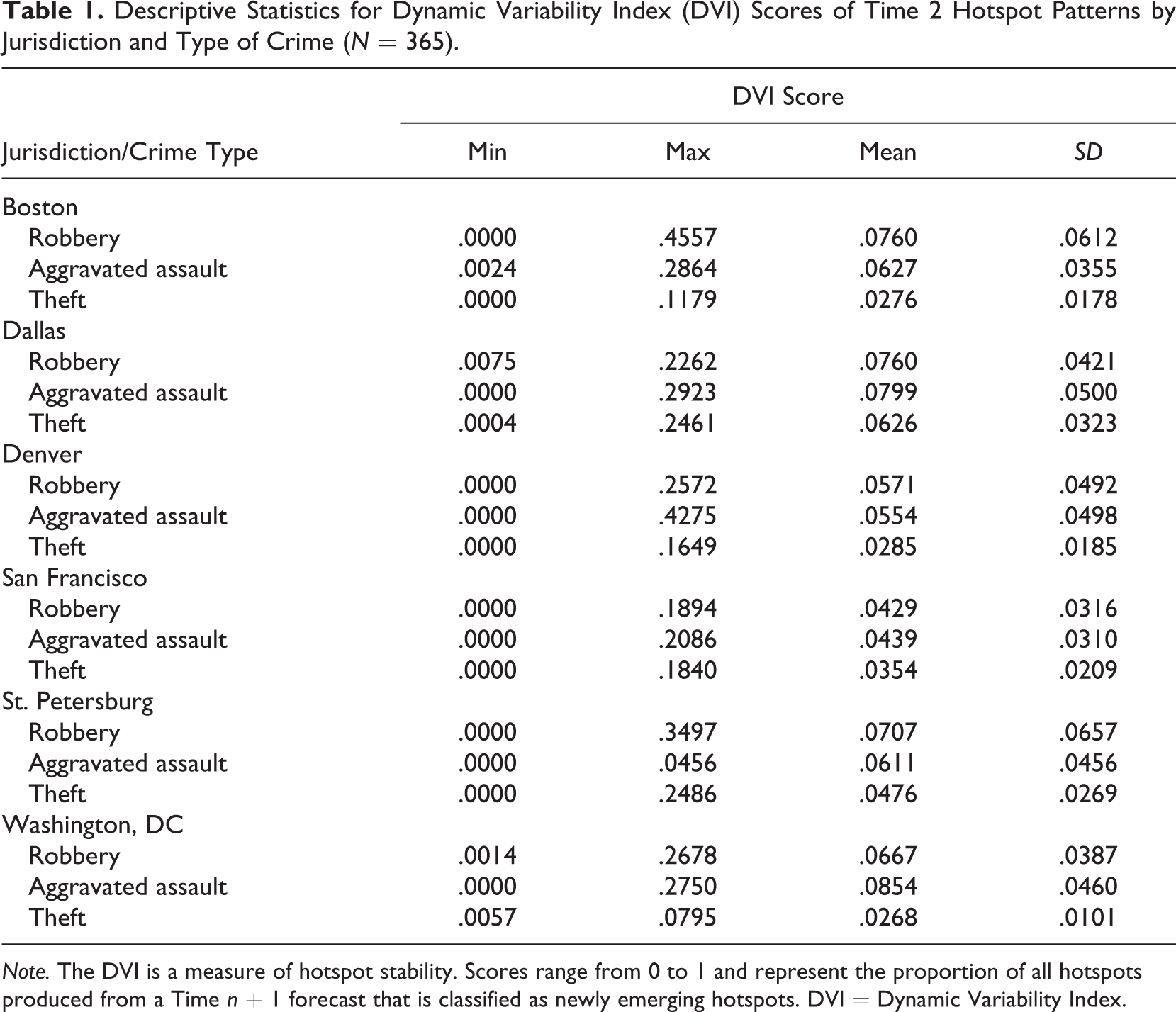
Note. The DVI is a measure of hotspot stability. Scores range from 0 to 1 and represent the proportion of all hotspots produced from a Time n + 1 forecast that is classified as newly emerging hotspots. DVI = Dynamic Variability Index.

Research Hypotheses

Answers to the current research questions were derived from testing a series of hypotheses related to crime pattern stability, based on micro-temporal forecasts. The specific research hypotheses tested in the current study are as follows:

Hypothesis 1: The dynamic variability of crime hotspot patterns, based on micro-temporal (i.e., daily) forecasts, is crime-type dependent.

Hypothesis 2: The dynamic variability of crime hotspot patterns, based on micro-temporal forecasts, differs between geographic locations.

Hypothesis 3: The dynamic variability of crime hotspot patterns, based on micro-temporal forecasts, varies by the interaction of crime type and jurisdiction.

Two-way between-group analysis of variance (ANOVA) was used to test these hypotheses, using a two-tailed test and a .05 α-level. Results are presented in the next section.

Results

Hotspot Stability and Crime Type

Results of the 3 × 6 ANOVA are presented in Table 2 and show that average DVI scores for daily crime patterns differ significantly by crime type, F(2, 6569) = 322.88, p < .001. However, pairwise comparisons for each crime type examined are presented in Table 3 and reveal significant differences in stability were not observed between all three types of crime patterns examined. For example, the average Time 2 DVI score for aggravated assault forecasts was .0267 higher (95% confidence interval [.0238, .0296]) than the average larceny Time 2 DVI score (d = .75). A similar pattern was observed for robbery and larceny, but significant differences were not observed between the two violent crimes examined. These findings provide some evidence in support of the first research hypothesis.

Table 2.

Results of a 3 × 6 ANOVA Showing the Main and Interaction Effects of Crime Type and Jurisdiction on Time 2 DVI Scores.

Source of Variation	SS	df	MS	F	p	η _p ²
Crime type	1.05	2	.52	322.88	<.001	.09
Jurisdiction	0.68	5	.14	84.53	<.001	.06
Crime type × Jurisdiction	0.43	10	.04	26.53	<.001	.04
Total	33.30	6,569

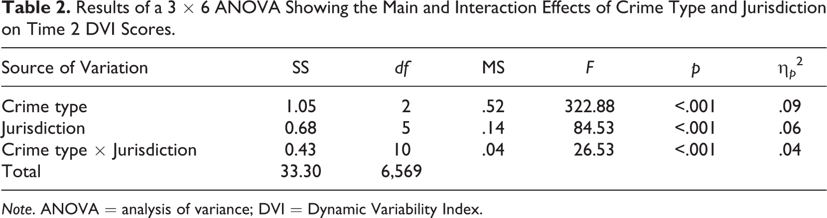
Note. ANOVA = analysis of variance; DVI = Dynamic Variability Index.

Table 3.

Pairwise Comparisons of Time 2 DVI Scores by Crime Type.

Crime Type	Mean Difference	SE	95% Confidence Interval		p
Crime Type	Mean Difference	SE	Lower Limit	Upper Limit	p
Robbery–aggravated assault	.0002	.0011	−.0027	.0031	1.00
Robbery–larceny	.0268	.0011	.0239	.0297	<.001
Aggravated assault–larceny	.0267	.0011	.0238	.0296	<.001

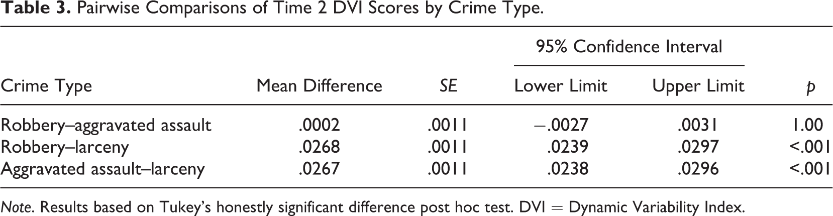
Note. Results based on Tukey’s honestly significant difference post hoc test. DVI = Dynamic Variability Index.

Hotspot Stability and Geographic Location

The main effect that geographic location (i.e., jurisdiction) has on Time 2 DVI scores is also presented in Table 2 and is generally supportive of the second hypothesis. Results show that with very few exceptions, differences in average DVI scores differ across the six jurisdictions studied, F(5, 6569) = 84.53, p < .001. Specifically, Time 2 DVI scores are statistically similar between Boston and St. Petersburg, Boston and Washington, DC, and St. Petersburg and Washington, DC; however, Time 2 DVI scores vary significantly for all other pairwise comparisons made, which are presented in Table 4. Most notably, hotspot patterns are significantly more stable in San Francisco than any other jurisdiction examined, whereas they are more fluid in Dallas than all other jurisdictions. Collectively, the findings indicate that characteristics of jurisdictions in which hotspot policing strategies are implemented (e.g., the city’s size, its urban density, street network, access to and use of public transportation, etc.) may influence the daily stability patterns associated with crime forecasts.

Table 4.

Pairwise Comparisons of Time 2 DVI Scores by Jurisdiction.

Jurisdiction	Mean Difference	SE	95% Confidence Interval		p
Jurisdiction	Mean Difference	SE	Lower Limit	Upper Limit	p
Boston–Dallas	−.0174	.0017	−.0225	−.0124	<.001
Boston–Denver	.0084	.0017	.0033	.0134	<.001
Boston–San Francisco	.0146	.0017	.0096	.0197	<.001
Boston–St. Petersburg	−.0044	.0017	−.0095	.0006	.156
Boston–Washington, DC	−.0042	.0017	−.0093	.0008	.213
Dallas–Denver	.0258	.0017	.0208	.0309	<.001
Dallas–San Francisco	.0321	.0017	.0270	.0371	<.001
Dallas–St. Petersburg	.0130	.0017	.0080	.0181	<.001
Dallas–Washington, DC	.0132	.0017	.0082	.0183	<.001
Denver–San Francisco	.0062	.0017	.0012	.0113	.004
Denver–St. Petersburg	−.0128	.0017	−.0178	−.0077	<.001
Denver–Washington, DC	−.0126	.0017	−.0176	−.0076	<.001
San Francisco–St. Petersburg	−.0190	.0017	−.0241	−.0140	<.001
San Francisco–Washington, DC	−.0188	.0017	−.0239	−.0138	<.001
St. Petersburg–Washington, DC	−.0002	.0017	−.0049	.0052	1.00

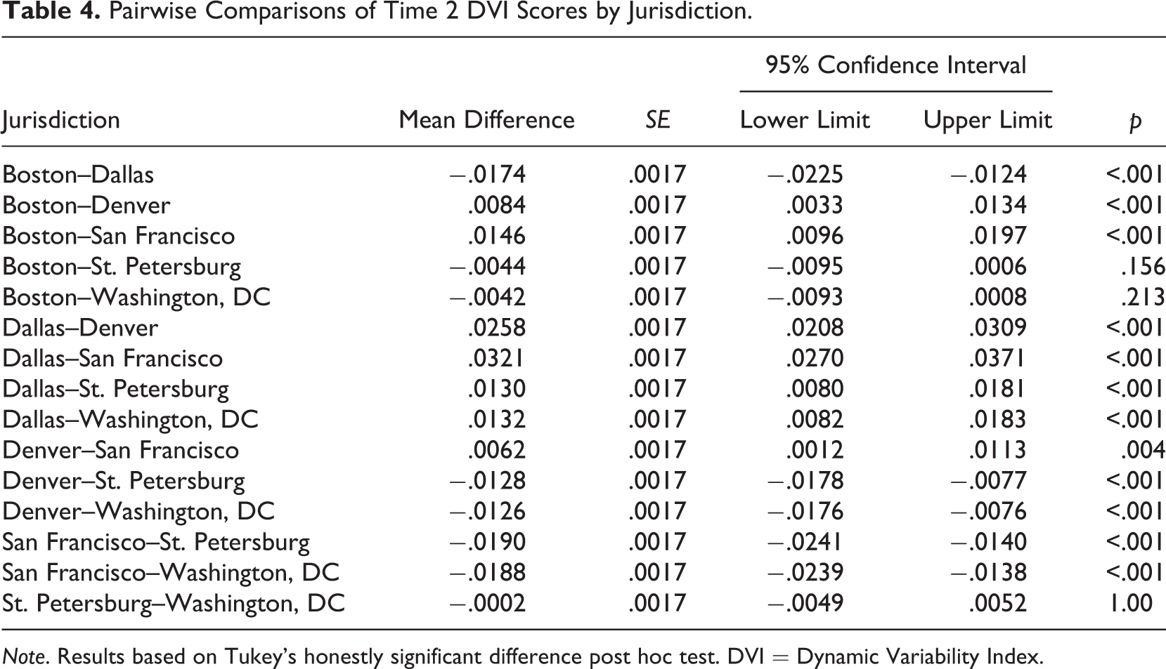
Note. Results based on Tukey’s honestly significant difference post hoc test. DVI = Dynamic Variability Index.

Interaction Effects

Table 2 also shows that Time 2 DVI scores are influenced significantly by the interaction between crime type and jurisdiction (F(10, 6569) = 26.53, p < .001); however, the percentage of variance in Time 2 DVI scores explained by the interaction effect is only about 4%. Figure 2 illustrates the relationship between crime type, jurisdiction, and crime pattern stability. The graph shows that robbery crime patterns are less stable in Boston, Dallas, and St. Petersburg than in Denver or San Francisco; aggravated assault hotspots in Washington, DC are less stable than in all other jurisdictions except Dallas; and larceny crime patterns are less stable in Dallas than in any other jurisdiction considered. Overall, these results provide evidence supporting the third research hypothesis, which states that the dynamic variability of crime hotspot patterns varies by the interaction of crime type and jurisdiction.

Figure 2.

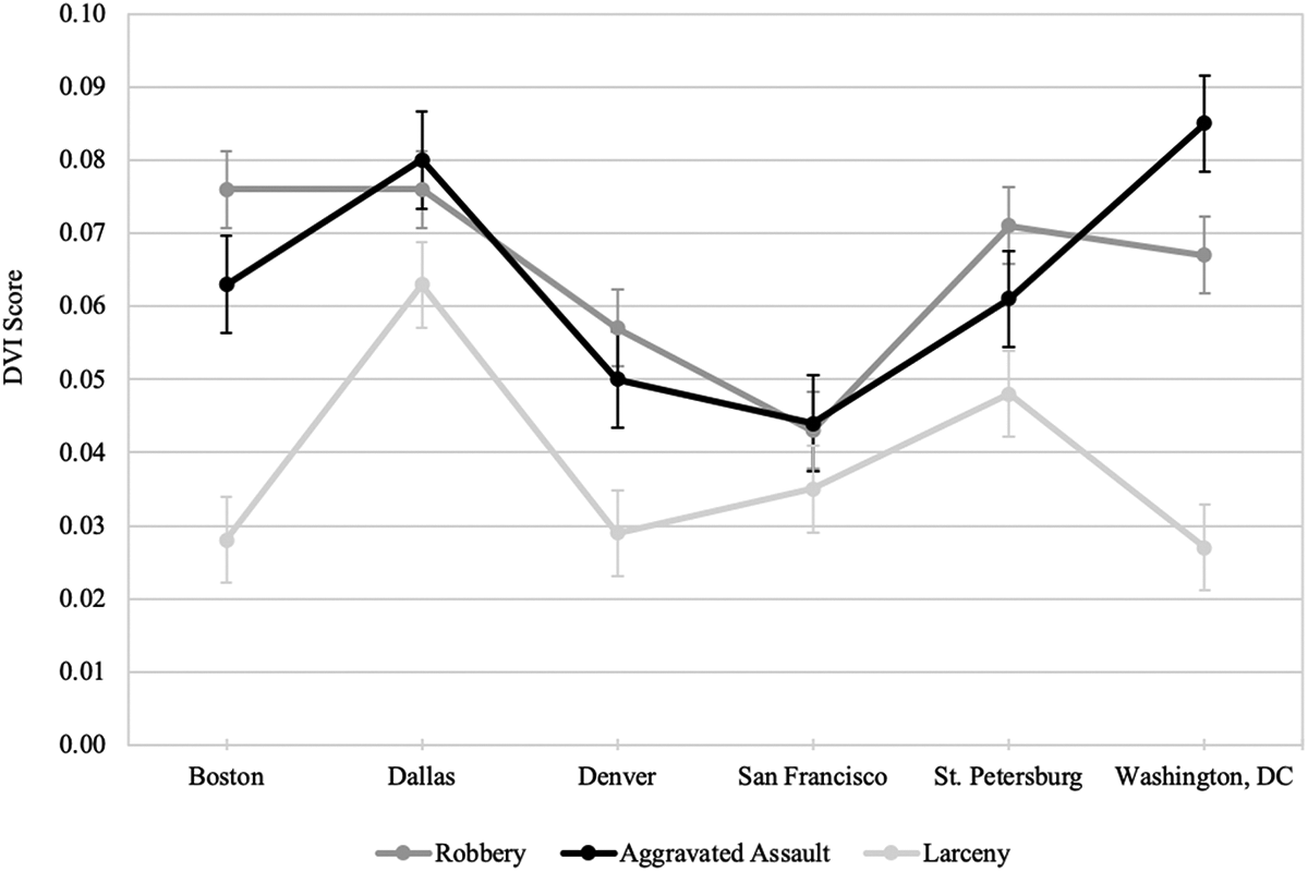
Average Time 2 DVI scores by crime type and jurisdiction. Note. Error bars are based on 95% confidence intervals. DVI = Dynamic Variability Index.

Discussion

The goal of the current investigation was to expand our empirical knowledge about the daily stability of crime hotspot forecasts. Three types of crime patterns were analyzed, based on incident location data produced from six U.S. law enforcement agencies. The stability of hotspot predictions for each crime type was examined every day, over a 1-year period; crime hotspot stability was measured using Adepeju et al.’s (2016) DVI. Answers to three research questions that guided this investigation are discussed in the remainder of this section.

First, the results from the current study provide empirical evidence that the stability of micro-temporal hotspot predictions is crime-type dependent. However, differences in average DVI scores were only observed between robbery and larceny hotspots and aggravated assault and larceny hotspots; they were not observed when DVI scores for robbery and aggravated assault hotspots were compared. These findings could be related to the relative frequency with which these incidents occur or the way in which the opportunities to commit these offenses change over short time intervals. Although identifying factors that could explain the daily stability of crime patterns for these types of hotspots is beyond the scope of the current investigation, future research should pursue this line of inquiry. Until we know more, however, it is recommended that analysts—particularly tactical crime analysts focused on daily crime problems—examine the fluidity of crime patterns as part of their agency’s hotspot policing intervention strategies. Furthermore, given the findings related to the first research question, this analysis should be undertaken separately for each crime type for which an intervention strategy is designed.

Second, the results from the current investigation provide empirical evidence that the daily stability of crime patterns varies by jurisdiction. Differences in crime pattern stability were observed between all jurisdictions studied, except between Boston and San Francisco, Boston and St. Petersburg, and St. Petersburg and Washington, DC. As noted previously, law enforcement agencies were selected purposively for this investigation, in part, because they differ in many ways that could influence crime hotspot patterns. These factors include the size of a jurisdiction’s population, the size of patrol areas, urban density, street network designs, and the availability and use of public transportation. Future research should be undertaken aimed at disentangling the relationship between characteristics of an agency’s jurisdictions and how it could influence crime pattern stability. Until then, given the current findings related to the second research question, analysts should be cognizant of the particular micro-temporal patterns of crime forecast stability within their own jurisdiction, as patterns for similar incidents in different jurisdictions may not produce similar stability patterns in their own. Assuming that these patterns are consistent across every jurisdiction would be a mistake that could diminish the effectiveness of hotspot policing efforts.

Third, the results from the current investigation provide empirical evidence that the daily stability of crime patterns is impacted significantly by the interaction between crime type and jurisdiction. For example, except in San Francisco, daily hotspot predictions associated with larcenies are more stable than patterns associated with robberies or aggravated assaults. Likewise, aggravated assault predictions are more fluid in Dallas and Washington, DC than in the other four jurisdictions studied. Finally, DVI scores for the three crime types examined in Boston and Washington, DC varied from one another significantly; however, Time 2 DVI scores for all three crime types were statistically similar in San Francisco. These findings underscore the importance of the interaction between crime type and jurisdiction on micro-temporal crime pattern stability. Therefore, in addition to the recommendations mentioned previously, analysts must be aware of the unique crime pattern stability signatures within their own jurisdictions and how the patterns of one type of crime compare to others. This is especially important if an agency routinely targets various types of crime hotspots for policing interventions. Understanding which crime patterns are more stable or fluid within a jurisdiction, relative to other crime patterns, can help guide existing hotspot policing strategies in ways that could maximize their benefits.

Answers to these three questions that guided the current study were derived from a relatively new approach to understanding crime hotspot patterns, which involved the creation and application of several algorithms. Unlike proprietary software and tools that lack transparency due to licensing agreements or trade secrets, models applied in the current study are freely available online (see Note 13). In addition to making the current research more transparent, providing access to these models and algorithms allows researchers and practitioners to replicate any aspect of the current investigation. This should be the standard in crime and place research, as it makes the contribution of an investigation more valuable. Future research should commit to a similar approach.

Limitations

Despite producing new empirical knowledge about the stability of micro-temporal crime forecasts, the current investigation is not without certain limitations. For example, the current study used incident location data for three crime types, collected from six law enforcement agencies. Although analysis of these data revealed important insights about crime pattern stability, patterns observed in the current study cannot be generalized to other crime types or to other jurisdictions. In addition, a single micro-temporal interval was used to produce hotspot forecasts (i.e., 1 day). It is unclear whether similar findings would be observed if different time intervals (i.e., 2, 5, or 7 days) were applied. Relatedly, only a single metric was used to measure forecast stability (i.e., the DVI), and other characteristics of crime patterns (i.e., compactness or predictive accuracy) were not considered. There could be trade-offs between the patrollability of crime patterns and their stability that the current study did not address. This is a noteworthy line of inquiry, but beyond the scope of the current investigation. Finally, prospective hotspot forecasts were made using a single method (i.e., KDE). Despite being one of the most popular and reliable methods used in crime hotspot mapping, it is not without its own limitations (see, Zambom and Dias, 2012, for a review), and different results could have been observed if different prediction methods were utilized. Regardless of these shortcomings, the current study has made a meaningful contribution to the extant literature and can be used to support analysts in their efforts to reduce and prevent crime within their communities. It has also generated more questions about crime pattern stability that should be investigated by future research.

Conclusions

Hotspot policing is a law enforcement strategy that can be used to reduce and prevent crime. These initiatives are guided by a fundamental truth: Crime is not randomly distributed in space and time. By targeting policing resources at particular places and at specific times, we can maximize the impact of our hotspot policing efforts within our communities. The current study adds to our understanding of how we can continue to support the efficiency and efficacy of these strategies by demonstrating how the stability of hotspot predictions made at micro-temporal intervals varies by crime type, jurisdiction, and the interaction between both.

Footnotes

Declaration of Conflicting Interests

The author declared no potential conflicts of interest with respect to the research, authorship, and/or publication of this article.

Funding

The author received no financial support for the research, authorship, and/or publication of this article.

ORCID iD

Timothy C. Hart

Notes

References

Adepeju

Cheng

Shawe-Taylor

Bowers

(2015, April 15–17). A new metric of crime hotspots for operational policing [Paper presentation]. 23rd Geographical Information Science Research UK Conference, Leeds, UK.

Adepeju

Rosser

Cheng

(2016). Novel evaluation metrics for sparse spatio-temporal point process hotspot predictions: A crime case study. International Journal of Geographical Information Science, 30(11), 2133–2154. https://doi.org/10.1080/13658816.2016.1159684

Andresen

M. A.

(2009). Testing for similarity in area-based spatial patterns: A nonparametric Monte Carlo approach. Applied Geography, 29, 333–345.

Andresen

M. A.

(2011). The ambient population and crime analysis. The Professional Geographer, 63(2), 193–212. https://doi.org/10.1080/00330124.2010.547151

Andresen

M. A.

Linning

S. J.

Malleson

(2017). Crime at places and spatial concentrations: Exploring the spatial stability of property crime in Vancouver BC, 2003-2013. Journal of Quantitative Criminology, 33(2), 255–275.

Anselin

(1995). Local indicators of spatial association–LISA. Geographical Analysis, 27(2), 93–115. https://doi.org/10.1111/j.1538-4632.1995.tb00338.x

Bailey

Gatrell

(1995). Interactive spatial data analysis. Longman Scientific & Technical.

Ball

G. H.

Hall

D. J.

(1970). A clustering technique for summarizing multivariate data. Behavioral Science, 12, 153–155.

Bender

(1962). Area-perimeter relations for two dimensional lattices. The American Mathematical Monthly, 69, 742–774.

10.

Boba

R. S.

(2016). Crime analysis with crime mapping (4th ed.). Sage.

11.

Bowers

K. J.

Johnson

S. D.

Pease

(2004). Prospective hot-spotting: The future of crime mapping? British Journal of Criminology, 44(5), 641–658. https://doi.org/10.1093/bjc/azh036

12.

Braga

A. A.

Andresen

M. A.

Lawton

(2017). The law of crime concentration at places: Editors’ introduction. Journal of Quantitative Criminology, 33, 421–426. https://doi.org/10.1007/s10940-017-9342-0

13.

Brantingham

P. J.

Brantingham

P. L.

(1984). Patterns in crime. Prentice Hall.

14.

Brantingham

P. J.

Brantingham

P. L.

(1991). Environmental criminology. Waveland Press.

15.

Brantingham

P. J.

Brantingham

P. L.

Andresen

M. A.

(2016). The geometry of crime and crime pattern theory. In Wortley

Townsley

(Eds.), Environmental criminology and crime analysis (2nd ed., pp. 119–136). Routledge.

16.

Caplan

J. M.

Kennedy

L. W.

(2010). Risk terrain modeling manual: Theoretical framework and technical steps of spatial risk assessment. Rutgers Center on Public Security.

17.

Caplan

J. M.

Kennedy

L. W.

Miller

(2011). Risk terrain modeling: Brokering criminological theory and GIS methods for crime forecasting. Justice Quarterly, 28(2), 360–381. https://doi.org/10.1080/07418825.2010.486037

18.

Chainey

(2013). Examining the influence of cell size and bandwidth size on kernel density estimation crime hotspot maps for predicting spatial patterns of crime. Bulletin of the Geographical Society of Liege, 60, 7–19.

19.

Chainey

Tompson

Uhlig

(2008). The utility of hotspot mapping for predicting spatial patterns of crime. Security Journal, 21(1), 4–28. https://doi.org/10.1057/palgrave.sj.8350066

20.

Clarke

R. V

(1995). Situational crime prevention. In Tonry

Farrington

D. P.

(Eds.), Building a safe society: Strategic approaches to crime prevention, vol. 19 of Crime and Justice: A review of research. University Press.

21.

Cohen

L. E.

Felson

(1979). Social change and crime rate trends: A routine activity approach. American Sociological Review, 44(4), 588–608. https://doi.org/10.2307/2094589

22.

Drawve

(2016). A metric comparison of predictive hot spot techniques and RTM. Justice Quarterly, 33(3), 369–397.

23.

Environmental Systems Research Institute. (2016). ArcGIS Desktop: Release 10.5. [Computer software]. https://desktop.arcgis.com/en/

24.

Felson

Eckert

(2019). Crime and everyday life: A brief introduction (6th ed.). Sage.

25.

Fielding

Jones

(2011). Disrupting the optimal forager: Predictive risk mapping and domestic burglary reduction in Trafford. Greater Manchester. International Journal of Police Science & Management, 14(1), 30–41.

26.

Getis

Ord

J. K.

(1992). The analysis of spatial association by use of distance statistics. Geographical Analysis, 24(3), 189–206. https://doi.org/10.1111/j.1538-4632.1992.tb00261.x

27.

Groff

E. R.

Taniguchi

(2018). Micro-level policing for preventing near repeat residential burglary: Final monograph. Police Foundation.

28.

Hart

Zandbergen

(2014). Kernel density estimation and hotspot mapping: Examining the influence of interpolation method, grid cell size, and bandwidth on crime forecasting. Policing: An International Journal of Police Strategies & Management, 37(2), 305–323. https://doi.org/10.1108/PIJPSM-04-2013-0039

29.

Hartigan

J. A.

(1975). Clustering algorithms. John Wiley & Sons.

30.

Jeffery

C. R.

(1971). Crime prevention through environmental design. Sage.

31.

Johnson

S. D.

(2017). Crime mapping and spatial analysis. In Wortley

Townsley

(Eds.), Environmental criminology and crime analysis (2nd ed., pp. 199–223). Routledge.

32.

Johnson

S. D.

Bowers

K. J.

(2004a). The burglary as a clue to the future: The beginnings of prospective hot-spotting. The European Journal of Criminology, 1, 237–255.

33.

Johnson

S. D.

Bowers

K. J.

(2004b). The stability of space-time clusters of burglary. British Journal of Criminology, 44, 55–65.

34.

Johnson

S. D.

Bowers

K. J.

Birks

Pease

(2009). Predictive mapping of crime by ProMap: Accuracy, units of analysis, the environmental backcloth. In Weisburd

Bernasco

Bruinsma

(Eds.), Putting crime in its place: Units of analysis in spatial crime research (pp. 171–198). Springs.

35.

Johnson

S. D.

Lab

S. P.

Bowers

K. J.

(2008). Stable and fluid hotspots of crime: Differentiation and identification. Built Environment, 34(1), 32–45.

36.

Lee

Gong

Shengwen

(2017). Exploring spatiotemporal clusters based on extended kernel estimation methods. International Journal of Geographical Information Science, 31(6), 1154–1177.

37.

Lemieux

A. M.

Felson

(2012). Risk of violent crime victimization during major daily activities. Violence and Victims, 27(5), 635–655. https://doi.org/10.1891/0886-6708.27.5.635

38.

Levine

(2008). The ‘hottest’ part of a hotspot: Comments on “the utility of hotspot mapping for predicting spatial patters of crime.” Security Journal, 21(4), 295–302. https://doi.org/10.1057/sj.2008.5

39.

Levine

(2015). CrimeStat: A spatial statistics program for the analysis of crime incident locations (Version 4.02) [Apparatus and software]. National Institute of Justice.

40.

McBratney

A. B.

deBruijter

J. J.

(1992). A continuum approach to soil classification by modified fuzzy k-means with extragrades. Journal of Soil Science, 43, 159–175.

41.

Mohler

G. O.

Short

M. B.

Brantingham

P. J.

Schoenberg

F. P.

Tita

G. E.

(2011). Self-exciting point process modeling of crime. Journal of the American Statistical Association, 106(493), 100–108. https://doi.org/10.1198/jasa.2011.ap09546

42.

Newman

(1972). Defensible space: Crime prevention through urban design. Macmillan.

43.

Ord

J. K.

Getis

(1995). Local spatial autocorrelation statistics: Distributional issues and an application. Geographical Analysis, 27(4), 286–306.

44.

Pease

Farrell

(2016). Repeat victimisation. In Wortley

Townsley

(Eds.), Environmental criminology and crime analysis (2nd ed., pp. 180–198). Routledge.

45.

Perry

W. L.

McInnis

Price

C. C.

Smith

S. C.

Hollywood

J. S.

(2013). Predictive policing: The role of crime forecasting in law enforcement operations. Rand Corporation.

46.

Pitney Bowes Software. (2016). MapInfo professional. Pitney Bowes.

47.

Ratcliffe

J. H.

(2002). Aoristic signatures and the spatio-temporal analysis of high volume crime patterns. Journal of Quantitative Criminology, 18, 23–43. https://doi.org/10.1023/A:1013240828824

48.

R Core Team. (2013). R: A language and environment for statistical computing. R Foundation for Statistical Computing. http://www.R-project.org/

49.

Silverman

B. W.

(1986). Density estimation for statistics and data analysis. Chapman & Hall.

50.

Spring

J. V.

Block

C. R.

(1989). STAC user’s manual. Illinois Criminal Justice Information Authority.

51.

Steenbeek

Weisburd

D. L.

(2015). Where the action is in crime? An examination of variability of crime across different spatial units in The Hague, 2001–2009. Journal of Quantitative Criminology, 32, 449–469.

52.

Thompson

H. R.

(1956). Distribution of distance to nth neighbour in a population of randomly distributed individuals. Ecology, 37, 391–394.

53.

Townsley

Homel

Chaseling

(2003). Infectious burglaries: A test of the near repeat hypothesis. The British Journal of Criminology, 43(1), 615–633. https://doi.org/10.1093/bjc/43.3.615

54.

Turner

M. G.

(1989). Landscape ecology: The effect of pattern on process. Annual Review of Ecology and Systematics, 20(1), 171–197. https://doi.org/10.1146/annurev.es.20.110189.001131

55.

Van Patten

I. T.

McKeldin-Coner

Cox

(2009). A microspatial analysis of robbery: Prospective hot spotting in a small city. Crime Mapping: A Journal of Research and Practice, 1(1), 7–32.

56.

Vandeviver

Steenbeek

(2019). The (in)stability of residential burglary patterns on street segments: The case of Antwerp, Belgium 2005–2016. Journal of Quantitative Criminology, 35(1), 111–133.

57.

Ward

J. H.

(1963). Hierarchical grouping to optimize an objective function. Journal of the American Statistical Association, 58, 236–244.

58.

Weisburd

(2015). The law of crime concentration and the criminology of place. Criminology, 53(2), 133–157. https://doi.org/10.1111/1745-9125.12070

59.

Weisburd

Majmundar

M. K.

(2018). Proactive policing: Effects on crime and communities. National Academies Press.

60.

Zambom

A. Z.

Dias

(2012). A review of kernel density estimation with applications to econometrics. International Econometric Review, 5, 20–42.