Disorder or Disadvantage: Investigating the Tension Between Neighborhood Social Structure and the Physical Environment on Local Violence

Abstract

A renewed interest in understanding the relationship of the built environment with neighborhood crime patterns has encouraged researchers to utilize novel methods (e.g., risk terrain modeling) to better examine the influence of environmental risk factors on types of crime. The current study engages with this research by operationalizing neighborhoods using Hipp and Boessen’s egohood strategy and using Drawve’s aggregate neighborhood risk of crime measure to assess the relationship of a neighborhood’s physical environment with its spatial vulnerability of experiencing a homicide. Findings demonstrate that the physical environment was a significant predictor of neighborhood homicide; however, social structural neighborhood characteristics were more important. This suggests crime prevention strategies like crime prevention though environmental design or blight remediation may provide prudent and straightforward methods to inhibit lethal violence in a community in the short run, but that addressing a neighborhood’s social structural characteristics may be more effective at reducing homicides in the long term.

Keywords

environmental criminology neighborhoods and crime risk terrain modeling egohoods homicide

Introduction

Municipalities across the country have increasingly sought to address the root causes of crime with strategies that target environmental factors associated with crime such as blight (Braga et al., 2015; Wilcox et al., 2018). The broader research on neighborhood correlates of crime has drawn upon several theoretical frameworks including the social disorganization framework, the broken windows thesis, crime pattern theory, and routine activity theory to explain neighborhood crime patterns. These frameworks differ regarding the specific predictors of higher neighborhood crime, but broadly speaking argue that neighborhood crime levels were a function of a combination of socioeconomic disadvantage as measured through population characteristics and opportunities to engage in crime measured through environmental risk factors (Wilcox et al., 2018). These frameworks were often assessed in competition with each other, which has led to questions about whether social characteristics of neighborhood populations and environmental factors (such as blight or disorder) were equal predictors of crime (Kim & Hipp, 2019; Sampson, 2012; Wilcox et al, 2018).

The discrepancies in findings were likely a function of variation in the operationalization of neighborhood characteristics but may also be due to how neighborhoods were conceptualized. For example, research on neighborhood correlates of crime operationalized neighborhoods through census-based areal units (i.e., tracts, block groups, or blocks; Hipp, 2007), community areas (Skogan, 1990), neighborhood clusters (Sampson & Raudenbush, 1999), a four-block radius of survey respondents (Rountree et al., 1994), and more recently egohoods (Hipp & Boessen, 2013; Kim & Hipp, 2019). The variation in the unit of analysis was potentially important for two reasons. First, neighborhood borders perceived by residents may not match well with administrative boundaries (Hipp & Boessen, 2013; Hipp, Wiliams & Boessen, 2018; Kirk & Laub, 2010). Second, recent neighborhood-level research discussed the modifiable areal unit problem (MAUP), which refers to the potential for relationships to operate differently depending on the unit of analysis used (Kim & Hipp, 2019; Tita & Radil, 2010; Vogel, 2016).

The current study draws upon the broad range of theories of neighborhood correlates of crime to examine whether social structural characteristics or environmental features of neighborhoods were more strongly associated with homicides in Baton Rouge, LA. We make several contributions to the research on neighborhood correlates of crime. First, we employ Drawve’s (2016; Thomas & Drawve, 2018) aggregate neighborhood risk of crime (ANROC), by way of Caplan and Kennedy’s (2016) risk terrain modeling (RTM), to examine the relationship of social structural characteristics and environmental features with homicide. Second, we operationalize neighborhoods using Hipp and Boessen’s (2013) egohood approach, which are created by drawing overlapping concentric buffers around census blocks. We chose egohoods over other types of areal units of analysis because they better approximate resident perceptions of neighborhood boundaries and therefore are more useful for assessing the relationship of localized phenomenon with violent crime (Hipp & Bates, 2018; Kim & Hipp, 2019). The use of egohoods helps us to engage with the MAUP because they provide a conceptual bridge across traditional census units including blocks, block groups, and tracts. Finally, we expand research on neighborhood correlates of violence in medium size cities.

Literature Review

The spatial concentration of violence in cities has been well established (MacDonald & Stokes, 2020; Sampson, 2012; Valasik et al., 2019; Wilcox et al., 2018). The most used explanations for the spatial concentration of violence included the social disorganization framework, geometry of crime/routine activity perspective, and the broken windows thesis (McDonald & Stokes, 2020; Sampson, 2012; Wilcox et al., 2018). These frameworks emphasize the importance of different aspects of neighborhoods, but all generally highlight the importance of population characteristics and opportunities for violence within neighborhoods.

The social disorganization framework highlighted the importance of the spatial distribution of population characteristics. Specifically, this framework argues crime and violence are spatially correlated with poverty, residential instability, and racial/ethnic heterogeneity because they lead to tenuous social ties that decrease the effectiveness of informal social control (Sampson, 2012; Shaw & McKay, 1942/1969). Recent assessments of this framework found community characteristics mediated the relationship of population characteristics with crime but continued to find higher levels of crime in neighborhoods characterized by concentrated disadvantage, residential instability and racial heterogeneity (Markowitz et al., 2001; Sampson, 2012).

While the social disorganization framework highlighted the importance of population characteristics for the spatial distribution of crime, the opportunities for crime research emphasized physical aspects of neighborhoods. P. J. Brantingham and Brantingham’s (1981; 1984) crime pattern theory holds that offenders and targets intersect during overlapping daily movements, providing opportunities for criminal acts to transpire. The overlapping daily movements of individuals and groups create pathways and relatively consistent schedules for offenders to exploit. The locations where individuals spend most of their time (work, school, home) were termed “nodes.” The combination of pathways and nodes make up an individual’s activity space (P. L. Brantingham & Brantingham, 1993). An offender’s most frequently traveled pathways and most frequently visited nodes make up their awareness space. P. L. Brantingham and Brantingham (1993, 1995) propose that awareness spaces and individuals’ paths and nodes with the greatest amount of traffic have the highest likelihood of criminal offending because potential offenders were more likely to be aware of opportunities in such spaces.

Crime pattern theory features substantial conceptual overlap with routine activity theory (Cohen & Felson, 1979; Felson, 1987) which stipulates criminal occurrences require the spatial and temporal intersection of a motivated offender, a suitable target and the absence of capable guardianship. This framework views criminal behavior as the outcome of decisions made after a cost–benefit analysis of the risks and rewards. The aggregation of decisions made by potential offenders and targets influence whether areas become crime generators or crime attractors. Crime generators are areas where potential offenders and victims intersect and feature characteristics that encourage potential offenders to believe criminal activity will be more successful (P. L. Brantingham & Brantingham, 1995). Crime attractors feature characteristics that entice potential offenders to travel to the area for the purpose of engaging in crime (P. L. Brantingham & Brantingham, 1995). Crime generators and attractors often occupy public or commercial spaces (P. L. Brantingham & Brantingham 1995; Valasik et al., 2019). Spaces that limit the offenders’ and targets’ mobility (through fences, buildings, rivers, or highways) create especially crime-prone areas termed as hotbeds (Weatherburn et al., 1999).

The broken windows/incivilities thesis emphasis by the physical appearance of neighborhoods by arguing fear of crime and occurrences of crime tend to be more common in neighborhoods characterized by signs of social (e.g., public arguments, loitering, public drunkenness) and physical disorder (e.g., graffiti, vandalism, neglect; Kelling & Coles, 1996; Taylor, 2001; Wilcox et al., 2018; Wilson & Kelling, 1982). Neighborhoods with greater signs of disorder were crime generators because the visibility of these incivilities discourage neighborhood residents from spending time outside in their neighborhood where they can act as guardians discouraging criminal activity (Kelling & Coles, 1996; Taylor, 2001; Wilcox et al., 2018). While conceptually appealing, empirical assessments of the relationship of neighborhood disorder with crime yielded mixed findings. Rountree et al. (1994) found neighborhood rates of burglary victimization in Seattle were higher in neighborhoods where incivilities were common. Further, a recent meta-analysis of the relationship of order maintenance policing, which focuses on reducing signs of social disorder, with crime found these strategies were associated with moderate declines in all types of crime (Braga et al., 2015). In contrast, Sampson and Raudenbush (1999) found the association of disorder with crime was spurious because both crime and disorder resulted from low levels of neighborhood collective efficacy. Gault and Silver (2008) questioned this conclusion and argued Sampson and Raudenbush’s (1999) finding that disorder was negatively associated with collective efficacy was consistent with Wilson and Kelling’s (1982) original statement. Overall, this suggests that disorder was associated with crime, but that the influence of disorder may be mediated by the characteristics of local communities.

Spatial vulnerability to homicide and RTM

Efforts to explain crime through the lenses of social disorganization and opportunity theories both recognize neighborhoods were interdependent. Land et al. (1990) used several areal units (i.e., cities, metropolitan areas, and states) and found that resource deprivation, population structure, and divorce rates consistently explained trends in homicide across units of analysis. Further, as predicted by the social disorganization framework, research found homicide rates were elevated in or near neighborhoods that featured concentrated disadvantage or moderate levels of residential instability (Giménez-Santana et al., 2018; McCall et al., 2010; Mears and Bhati, 2006). Research also found homicide clustered in specific areas of neighborhoods or cities (Braga et al., 2010; Rosenfeld et al., 1999; Valasik et al., 2019).

Drawing upon Kennedy and colleagues’ (2016) theory of risky places, a place’s vulnerability to experiencing a homicide, is the result of a combination of spatial features in the local environment which are able to significantly increase the risk of lethal violence occurring. Thus, homicides are more likely to transpire in places where vulnerability is greater. Specifically, where the independent environmental features that generate and/or attract homicides combine their spatial influence to make a place risky. Places at greater risk of experiencing a homicide do not solely emerge from spatial vulnerability but also their exposure to prior acts of lethal violence. A place may be more vulnerable to a homicide, but if a homicide has not transpired in that particular location, then the likelihood of a future act of lethal violence in that place is low. Conversely, a place vulnerable to a homicide that has repeatedly endured lethal violence is much more likely to experience homicides in the future. This vulnerability-exposure framework created by Kennedy and colleagues’ (2016) theory of risky places allows for not only a more nuanced understanding of where a homicide is going to occur but also highlights those environmental features contributing to a homicide which could be targeted as strategic points of intervention. Recent advances in spatial data analysis, particularly RTM which draws upon social and physical environment data to help identify places with greater vulnerability of experiencing a crime (e.g., homicide), can be used to test the propositions in the theory of risky places (Kennedy et al., 2016).

RTM was developed by Caplan and Kennedy (2016, p. 12) as a “statistically valid way to articulate vulnerable places” through the creation of risk of crime score for an area that is based upon the criminogenic characteristics present in the physical landscape, including the built environment. Specifically, RTM systematically identifies environmental risk factors associated with a type of crime in a particular area and assesses how the spatial influences of these risk factors collocate to increase an area’s vulnerability of experiencing future incidents of crime. RTM has been used to examine variation in aggravated assaults (Kennedy et al., 2016; Steinman et al., 2020; Thomas & Drawve, 2018), carjackings (Lersch, 2017), robberies (Caplan et al., 2017; Garnier et al., 2018; Kocher & Leitner, 2015), felonious battery to police officers (Caplan et al., 2014), gun-related crimes (Caplan et al., 2011; Drawve et al., 2014), and overall violent crime (Caplan et al., 2013; Drawve, 2016; Gerell, 2018). Most relevant to the current study was prior applications of RTM that examined the relationship of environmental risk factors with lethal violence (Connealy, 2019; Drawve, 2016; Gerell, 2018; Giménez-Santana et al., 2018; Kennedy et al., 2016; Thomas & Drawve, 2018; Valasik et al., 2019). While each of these studies found a unique combination of situational contexts and environmental risk factors successfully forecasted future acts of violence, a general pattern indicates the majority of a jurisdiction was not vulnerable to experiencing a homicide with only a few very high clusters being present. The extant literature’s diversity of research sites and outcome variables showcases the robustness of the Caplan and Kennedy’s (2016) theory of risky places’ three propositions. RTM provides a systematic approach to better understand where “social processes responsible for ‘neighborhood effects’” related to homicide transpire and allow local stakeholders, policy makers, and law enforcement to tailor responses to these criminogenic areas (Tita & Greenbaum, 2009, p. 167).

Neighborhood characteristics for the risk of crime

The broad research on neighborhood correlates of crime argued neighborhood crime was a function of population characteristics (social disorganization) or opportunities to engage in crime (environmental characteristics; Drawve, 2016; MacDonald et al., 2019; Piza et al., 2016; Sampson, 2012). Together, these explanations suggest population characteristics and physical neighborhood features were both important predictors of neighborhood crime, but previous research produced mixed findings which was more important (Rosenfeld et al., 2007; Sampson, 2012; Thomas & Drawve, 2018; Wilcox et al., 2018). To address these disparities in the literature, Drawve’s (2016, p. 89) developed the ANROC measure, a novel approach that measured the vulnerability to violent victimization at the neighborhood level “by simultaneously examining the influence of social and demographic factors as well as characteristics of the built environment.” The creativeness in the ANROC measure was that it linked with early research on the ecological correlates of crime focusing on the combined influence of population dynamics and land usage (Jacobs, 1961; Suttles, 1972). Thus, the use of the ANROC measure is more comprehensive, enhancing the application of RTM to not solely rely on measures of the built environment but also able to incorporate the social structural aspects of a community to better ascertain which characteristics were more strongly associated with the risk of violent victimization for a neighborhood (Drawve, 2016; Giménez-Santana et al., 2018; Thomas & Drawve, 2018). The current study utilizes Drawve’s (2016) ANROC measure to assess the importance of population characteristics and an aggregate measure of a neighborhood’s spatial vulnerability to crime based on the environmental risk factors forecasted by RTM.

Current Study

A renewed interest in the association of environmental factors with crime among policy makers has led to questions about the effectiveness of policies grounded in the combination of environmental explanations discussed prior. This includes policies such as zero-tolerance policing and encouraged a reinterpretation of the importance of physical environment (e.g., abandoned property) as focal point of intervention (Klinenberg, 2018). Furthermore, there remains a tension in the criminological literature about whether neighborhood crime levels were more heavily influenced by social disorganization of the local population or by physical features of neighborhoods associated with increased opportunities to engage in crime, such as signs of disorder (Rosenfeld et al., 2007; Sampson, 2012; Thomas & Drawve, 2018; Wilcox et al., 2018). The current study builds upon this research by incorporating two novel techniques to examine whether social structural characteristics of neighborhoods or features of the physical environment better predict future acts of lethal violence.

Hipp (2007) contends that the “best” areal unit for analyzing neighborhood crime patterns is based upon the issue being examined. Hipp and Boessen (2013) developed the egohood approach to more accurately capture an areal unit that matched with activity patterns of local residents. Similar to Hipp and Boessen (2013), we created egohood areas in Baton Rouge by using a half-mile buffer around each census block.

Additionally, we use RTM and employ Drawve’s (2016; Thomas & Drawve, 2018) ANROC measure, which better captures a neighborhood’s level of risk based upon features of the physical environment. RTM is an increasingly favored approach to forecasting areas that are spatially vulnerable to experiencing future criminal acts due to its ability to incorporate social and physical features of the environment and not rely solely upon prior criminal events (e.g., hot spot mapping [kernel density estimation], near repeat analyses) to anticipate future criminal acts (i.e., homicide; see Drawve, 2016; Dugato, 2013). While it is possible to include prior criminal events or kernel density estimation in RTM, it is not necessary or reliant upon their inclusion to produce reliable and precise forecasts (Drawve, 2016). Another practical benefit of RTM is that moving beyond the prior criminal events and focusing on the built environment provides a variety of points of intervention that do not rely only on policing efforts to inhibit crime but utilizes local businesses, nonprofits, and government agencies to alter areas vulnerability to crime (see Drawve 2016; MacDonald et al., 2019). Additionally, the avoidance of using prior criminal events avoids incorporating any potential bias or beliefs of police officers opaque in the crime data that could infringe upon the constitutional protections of citizens (see Ferguson, 2019; Koss, 2015).

In terms of better understanding patters of homicide, several recent studies utilized RTM across a variety of areal units (Connealy, 2019; Dugato et al., 2020; Giménez-Santana et al., 2018; Valasik, 2018; Valasik et al., 2019). The RTMDx Utility was used in these studies to identify which environmental risk factors were significantly associated with lethal violence and discern the spatial influence of those risk factors. Building on these studies application of RTM we average relative risk score (RRS) for micro units situated by the RTMDx Utility to calculate an ANROC measure, consistently calculated by prior research as the micro units situated within a census tract (Drawve, 2016; Thomas & Drawve, 2018). Given our operationalization of neighborhoods as egohoods, we instead average the RRS values for the micro units located within an egohood. We then evaluated the predictive value through stepwise negative binomial regressions to ascertain social structural characteristics or the ANROC measure had greater explanatory power in assessing where homicides were more likely to transpire.

Data and Methods

Research site

Baton Rouge is the capital and second largest city in Louisiana, behind New Orleans, with an approximate population of 228,694 residing in 57 community-designated neighborhoods (Priola & Kron, 2018; U.S. Census Bureau, 2017). Slightly more than half of Baton Rouge’s residents are Black (54.9%) with White residents making up just over a third (36.6%). Only about a third (32.3%) of residents 25 years and older have a received their bachelor’s degree. There is a substantial amount of residential mobility with just less than a fifth (18.8%) of residents residing at an address that differs from the previous year. Additionally, only half (49.5%) of residents own their home. More than a quarter (26%) of residents live under the poverty line with median household income in 2016 of $39,969, which is $17,000 below the national median income. The unemployment rate (8.8%) is almost double the national average (4.9%). Baton Rouge also has higher than average income inequality which is reflected in a Gini coefficient (0.53) that was more than 1.6 standard deviations above the national average (0.48; U.S. Census Bureau, 2017).

Patterns of violence have fluctuated in Baton Rouge over the past 30 year, but it remains one of the more violent cities in the United States (Johnson, 2013; Thomas, 2017) and continues to occupy a top spot among state per capita murder rates (Federal Bureau of Investigation [FBI], 2016; Lane, 2017). The city has hosted several interventions to curb the excessive levels of violence including the Partnership to Reduce Juvenile Gun Violence Program between 1997 and 1999 (Sheppard et al., 2000) and the Baton Rouge Area Violence Elimination Project (BRAVE), a local version of Operation Ceasefire, which aimed to reduce group-based violence between 2012 and 2015 (Barthelemy et al., 2016). The consistent levels of elevated violence make Baton Rouge an ideal research site to investigate the competing relationships between social structural composition and physical landscape features and lethal violence. As the city limits of Baton Rouge, other than the Mississippi River on the western boundary, are porous the current study includes all zip codes that intersect with the city limits and those contained within (see Valasik et al., 2019). For brevity, the study area is subsequently referred to simply as Baton Rouge.

Data sources

The current study utilizes four data sources. First, all known homicides that took place in East Baton Rouge Parish in 2016 and 2017 were compiled from the East Baton Rouge District Attorney’s Office. In 2017, East Baton Rouge parish experienced 125 homicides, 111 of which transpired within the study area (i.e., Baton Rouge). Second, XY-coordinate data obtained from the East Baton Rouge Parish GIS Open Data Map Portal identified blighted properties, bus stops, parks, and public high schools (Priola & Kron, 2018). Third, XY-coordinate data for all other spatial risk factors (e.g., banks/credit unions, bars/nightclubs, service stations, etc.) were acquired from Infogroup (http://www.infogroup.com), a commercial and residential information provider (see Caplan et al., 2017; Piza et al., 2016, 2018). Finally, block group level census measures were collected from the 2013–2017 American Community Survey 5-Year Estimates (Manson et al., 2019).

Egohoods

Much of the research on neighborhood correlates of crime analyzed variation in among administrative units such as census blocks or tracts, but several studies utilized smaller units including police beats or street segments (Braga et al., 2015; Hipp, 2007; Kim, 2016; Kim & Hipp, 2017). An often-discussed limitation of such areal units was that they did not match with resident perceptions of neighborhood boundaries (i.e., cognitive map) or reflect areas of potential interaction with offenders (Hipp & Boessen, 2013; Kim & Hipp, 2019). Hipp and Boessen’s (2013: 299) egohood approach corrects for this by constructing neighborhoods through a spatial technique where circles were drawn around every census block within a given radius. All blocks within the identified radius or that intersect the drawn circle were classified as part of an egohood. Figure 1 provides a hypothetical example of what this looks like. Each of the cells in Figure 1 represent a census block. Egohoods average the values of a variable for a given cell and all cells within a given radius to create an egohood version of a variable. So, the egohood vacancy rate for Cell 11 would be calculated by averaging the vacancy rate of Cells 6, 7, 8, 10, 11, 12, 14, 15, and 16. In comparison, the egohood vacancy rate of Cell 4 would be calculated by averaging the vacancy rates of Cells 3, 4, 7, and 8.

Figure 1.

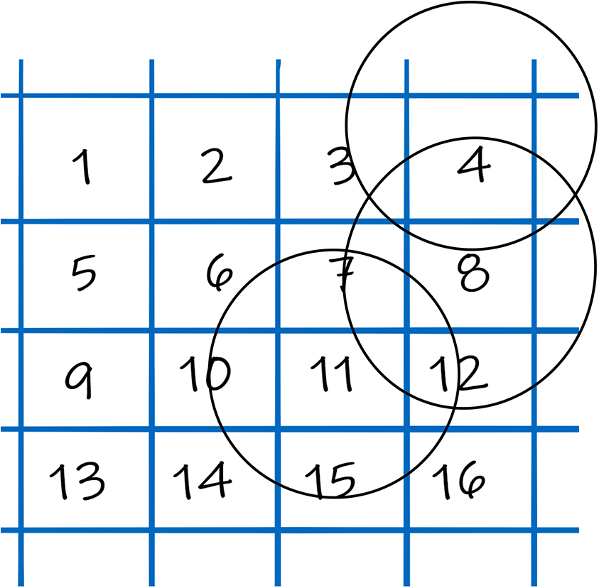
Example of egohoods.

In their foundational study on egohoods, Hipp and Boessen (2013) created egohoods based upon ¼, ½, and ¾ mile radii, but note that the ½ mile radius egohoods were closer approximations to census tracts boundaries most frequently used in research on neighborhood correlates of crime. Therefore, we used the ½ mile radius threshold when creating the current study’s egohoods. Hipp and Boessen (2013) found egohoods better represented how residents describe their local communities and engaged in their daily travel patterns and routine activities within these circumscribed environments (see also Hipp & Bates, 2018; Hipp & Williams, 2020).

Dependent variable

The dependent variable for the current study consists of all known homicides that took place in Baton Rouge during 2017. Information about all known homicides was provided by the East Baton Rouge District Attorney’s Office. We examined variation in homicide because homicide events are a well-documented and consistently tracked type of offense. While definitions of other crime types may vary across jurisdictions, the characteristics and definition of homicide remain constant. Furthermore, homicide’s position at the top of the FBI’s hierarchy rule assured that it would be recorded in official statistics even if it occurred in combination with another type of crime. All 111 incidents of homicide were geocoded and offset 20 ft from the street centerline using ArcGIS 10.6.1. Homicide counts were then aggregated to the egohood level.

Social structural disadvantage

Our study is grounded in several theories of neighborhood crime, but it is not intended to be a test of any of these frameworks. The specifics of these theories highlight the importance of different aspects of neighborhoods, but the common themes among these frameworks were that crime was more likely to occur in disadvantaged neighborhoods where social controls that discourage crime tend to be weaker (Sampson, 2012; Shaw & McKay 1942/1969; Wilcox et al., 2018). Hipp and Boessen (2013) argued that blocks were the best unit to base egohoods upon. This greatly limited our ability to utilize more conventional measures of neighborhood social structure such as concentrated disadvantage or residential mobility. Therefore, we replicated the measures used by Hipp and Boessen (2013) on egohoods as units of analysis for the current study.

Our measures of neighborhood disadvantage include the percent vacant units, the percent owner-occupied units, population density, percent of residents ages 15–29, and Black–White segregation. In addition to replicating Hipp and Boessen (2013), these measures were selected because they have been widely used in research on neighborhood correlates of violent crime (Hipp & Boessen 2013; Light & Thomas, 2019; Peterson & Krivo, 2010a; Valasik et al., 2017). We used the Geo-Segregation Analyzer to create a measure of Black–White entropy (Apparicio et al., 2013). We limited our segregation measure to Black and White residents because census statistics indicate about 54% of the population of Baton Rouge were Black, 36% were White, and the remaining 10% were composed of several other racial groups (U.S. Census Bureau, 2017).

We controlled for neighborhood economic environment with measures of absolute and relative economic inequality because previous research found these characteristics to be associated with conventional opportunities for economic gain and offender motivation (Hipp, 2007; Hipp & Boessen, 2013; Tita & Griffiths, 2005). Information about household income was not available at the block level, so we replicated Hipp and Boessen’s (2013: 300) decision to then create measures of economic inequality at the block level. Specifically, median household income was used to control for absolute economic inequality, and the standard deviation of the logged median household income was used to measure relative economic inequality across neighborhoods.

Physical environment

Eighteen spatial risk factors were identified and included in the RTM to assess the relationship of built environment with homicide. These potential risk factors include banks/credit unions, bars/cocktail lounges, blighted properties, bus stops, convenience stores,¹ food markets, fringe banks,² laundromats, liquor stores, parks, public high schools, public housing, restaurants, recreational centers, service stations, and tobacco/vape shops. The inclusion of these environmental risk factors was guided by personal knowledge of the city of Baton Rouge and the extant literature (Bernasco & Block, 2011; P. L. Brantingham & Brantingham, 1995; Drawve, 2016; Gerell, 2018; Valasik et al., 2018). To discern the spatial influence that these 18 environmental risk factors have on the risk of being a victim of a homicide, the RTM requires an outcome event. The outcome measure used in the current study is the location of homicides from the previous year. Data from 2016 were used to identify the spatial operationalization of features in the built environment impacting homicide and determine the risk associated with these spatial features (see Thomas & Drawve, 2018). Prior homicides were not utilized by the RTM to predict future crime, only environmental risk factors.

Of the 79 homicides that occurred in East Baton Rouge Parish in 2016, 71 transpired within the research site. All homicides were geocoded and offset 20 ft from the street centerline. The RTMDx Utility, created by the Rutgers Center on Public Safety, was employed to conduct this study’s RTM analysis (Caplan et al., 2013). RTM systematically discerns the appropriate operationalization of each included risk factor, determines the model type (Poisson or negative binomial) and ascertains the spatial risk factors that statistically influence outcome variables (i.e., homicide) in an area (Caplan & Kennedy, 2016; Heffner, 2013). The spatial influence for any risk factor remains geographically restrained to just a few city blocks (Caplan & Kennedy, 2016; Kennedy et al., 2011). The present study used the average block length as the areal unit of analysis. For the city of Baton Rouge this is 500 ft (as measured by ArcGIS 10.6.1). A grid of 98,702 cells, 500 ft × 500 ft, covering the research site, was then created. A penalized regression model was used by the RTMDx Utility with homicide counts serving as the dependent variable and the specified environmental risk factors as the independent variables. Across each of 98,702 cells, the RTMDx Utility ascertains whether a cell was located in a specified distance of a risk factor (i.e., proximity) or in a highly concentrated area of a risk factor (i.e., density). We sought to discern which environmental risk factors were positively associated with homicide (i.e., the dependent variable), or increased risk of homicide, so an “aggravating” model was used instead of a “protective” model that infers that the risk factors have a negative correlation with the homicide location, or lowers the amount of risk (Caplan et al., 2013). We set the spatial influence parameter at the maximum of four blocks (2,000 ft) and tested all included risk factors at half-block increments (i.e., 1/2 block [250 ft], 1 block [500 ft], 11/2 blocks [750 ft], 2 blocks [1,000 ft]).

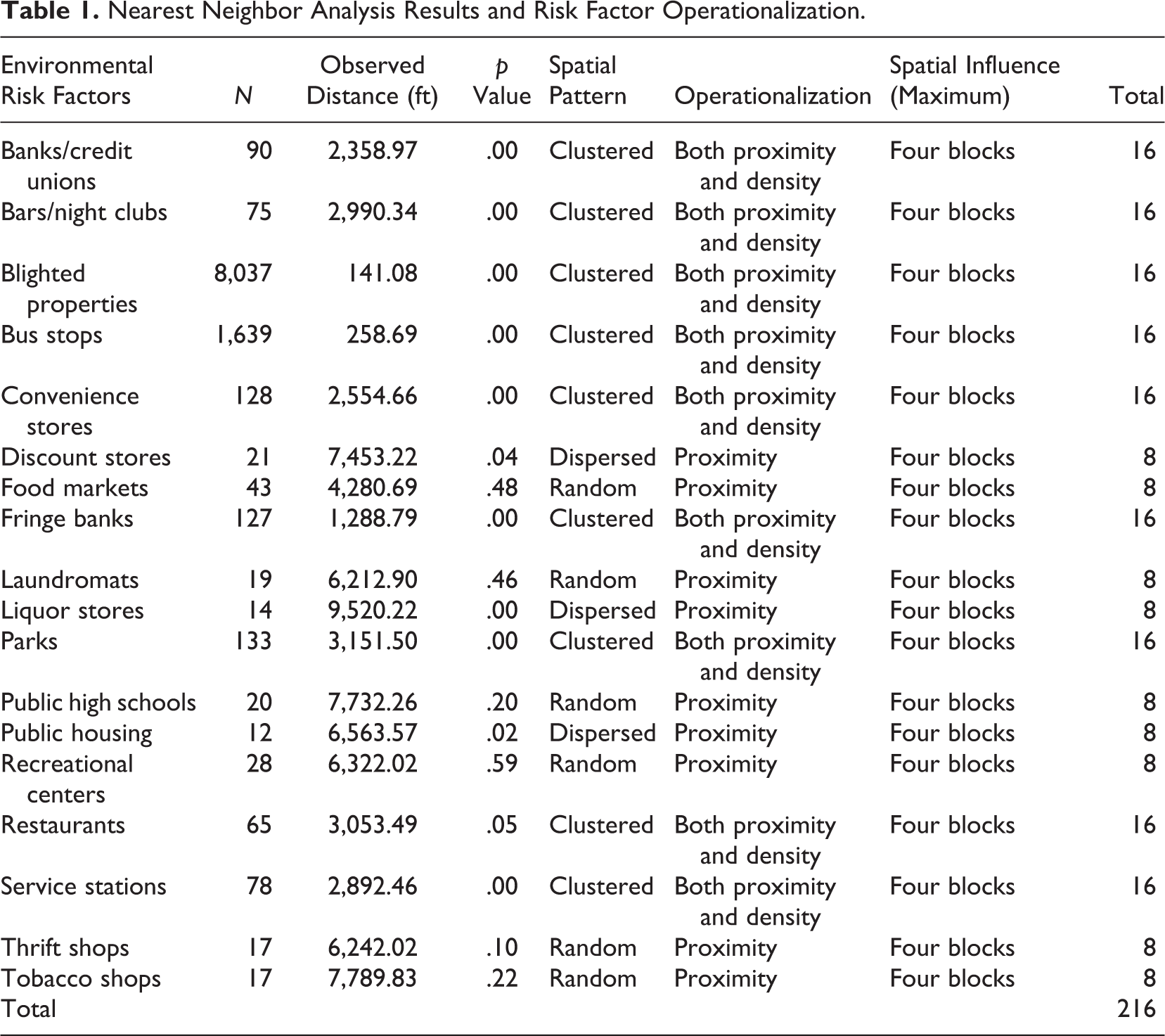
Caplan and Kennedy (2016) suggested conducting a nearest neighbor analysis for each spatial risk factor to assess their spatial operationalization.³ The results of these analyses are recorded in Table 1 along with operationalization parameter that corresponds with test outcomes. Caplan and Kennedy (2016) recommended operationalizing spatial risk factors that both significantly cluster and had a mean distance less than or equal to the nearest neighborhood threshold as both density and proximity. Those spatial risk factors whose observed mean distances were greater than the nearest neighborhood threshold or did not significantly cluster were operationalized only as proximity. Based upon the nearest-neighbor analysis, nine locations were tested in relation to only proximity as there were not enough across the city to cluster. Once the data were inputted and the operationalization parameters were decided, the RTMDx Utility examined each potential environmental risk factors relationship to the location of 2016 homicides, then ascertained what was the best fitting model derived from the risk factors identified as significant. The operationalization of the 18 environmental risk factors produced 216 total iterations (see Table 1). The RTMDx Utility utilizes a cross-validation procedure to overcome any spurious associations when a model includes a large number of variables by generating a penalized Poisson regression model where variables are considered for inclusion in a model when they have a nonzero coefficient (see Heffner, 2013). The model with the lowest Bayesian information criterion (BIC) score is considered to be the most appropriate following a stepwise regression where variables significant at the 0.05 level are selected (Heffner, 2013). For this study, the end product is an output with environmental risk factors that significantly relate to homicide, their appropriate operationalization and a value of their relative risk (see Heffner, 2013, for details on the statistics steering the RTMDx process).

Table 1.

Nearest Neighbor Analysis Results and Risk Factor Operationalization.

Environmental Risk Factors	N	Observed Distance (ft)	p Value	Spatial Pattern	Operationalization	Spatial Influence (Maximum)	Total
Banks/credit unions	90	2,358.97	.00	Clustered	Both proximity and density	Four blocks	16
Bars/night clubs	75	2,990.34	.00	Clustered	Both proximity and density	Four blocks	16
Blighted properties	8,037	141.08	.00	Clustered	Both proximity and density	Four blocks	16
Bus stops	1,639	258.69	.00	Clustered	Both proximity and density	Four blocks	16
Convenience stores	128	2,554.66	.00	Clustered	Both proximity and density	Four blocks	16
Discount stores	21	7,453.22	.04	Dispersed	Proximity	Four blocks	8
Food markets	43	4,280.69	.48	Random	Proximity	Four blocks	8
Fringe banks	127	1,288.79	.00	Clustered	Both proximity and density	Four blocks	16
Laundromats	19	6,212.90	.46	Random	Proximity	Four blocks	8
Liquor stores	14	9,520.22	.00	Dispersed	Proximity	Four blocks	8
Parks	133	3,151.50	.00	Clustered	Both proximity and density	Four blocks	16
Public high schools	20	7,732.26	.20	Random	Proximity	Four blocks	8
Public housing	12	6,563.57	.02	Dispersed	Proximity	Four blocks	8
Recreational centers	28	6,322.02	.59	Random	Proximity	Four blocks	8
Restaurants	65	3,053.49	.05	Clustered	Both proximity and density	Four blocks	16
Service stations	78	2,892.46	.00	Clustered	Both proximity and density	Four blocks	16
Thrift shops	17	6,242.02	.10	Random	Proximity	Four blocks	8
Tobacco shops	17	7,789.83	.22	Random	Proximity	Four blocks	8
Total							216

The RTMDx also produced an RRS for each of 98,702 cells in the research site. When the spatial influence of significant environmental risk factors overlap, a cell’s RRS will reflect this convergence. Thus, it is possible for environmental risk factors to independently influence the risk of being victim of a homicide or for that risk to be compounded when multiple environmental risk factors spatial influence overlaps. The best model identified by the RTMDx Utility was a negative binomial regression model for analyzing the number of homicides in 2016. As Table 2 shows, of the 18 potential environmental risk factors for this analysis, the RTMDx Utility ascertained that only two of those risk factors were significant for homicide in Baton Rouge: the concentration of blighted properties and the proximity to a convenience stores. The relative risk values and the distance at which these two environmental risk factors spatially influenced crime varies. The concentration of blighted properties within a two in a half block radius (i.e., 1,250 ft) elevated the risk of being a victim of a homicide by 13 times (12.613) compared to the least risky areas of Baton Rouge, the vast majority of the city. Similarly, being within a three in a half block radius (i.e., 1,750 ft) of a convenience store elevated the risk of being victimized in a homicide more than five-fold (5.467) compared to the least risky areas of Baton Rouge (see Valasik et al., 2018, for greater detail on the spatial influence of these risk factors). Even though a number of places within Baton Rouge exhibit some level of risk of experiencing a homicide, it was the spatial confluence of these two particular environmental risk factors, the proximity to convenience stores and the concentration of blighted properties that significantly elevated the risk of particular spaces.

Table 2.

The Risk Terrain Model With the Best Fit for Homicide.

Environmental Risk Factors	Spatial Influence (ft)	Operationalization	Coefficient	Relative Risk Value
Blighted properties	1,250	Density	2.535	12.613
Convenience stores	1,750	Proximity	1.699	5.467
Intercept	—	—	−8.600	—

Note. All variables included in the model demonstrate a p value of ≤ .001. Model: Negative binomial type II; BIC: 974.79.

In contrast, the other 16 environmental risk factors included in the RTMDx utility were not statistically associated with occurrences of homicide in Baton Rouge and were not included in subsequent analyses (see Caplan & Kennedy, 2016). While the inclusion of these environmental risk factors was based on the existing RTM literature and personal knowledge their convergence with each other, with blighted properties, or with convenience stores did not indicate any spatial influence with homicide. Furthermore, Valasik and colleagues (2019) testing to the predictive capacity of the RTM confirmed the robustness of the confluence of these two environmental risk factors at forecasting future homicides. RTM stresses that a unique combination of situational contexts and environmental risk factors converge for any particular type of crime in any particular jurisdiction, what Barnum and colleagues (2017) refer to as the “crime kaleidoscope.” As such, every RTM analysis of a crime type in a particular jurisdiction will reveal unique combinations of environmental risk factors and situational contexts that result in a distinct operationalization of spatial characteristics associated with that particular type of crime (see Connealy, 2019).

The RTMDx Utility designated the RRS to micro units (i.e., 500 ft × 500 ft cells). This facilitated the aggregation to more meaningful areal units (e.g., block group, egohood). This aggregation produced the average neighborhood level of risk of being victimized value (ANROC) based upon the significant environmental risk factors. For the current study, the ANROC value was calculated as the average risk score for the raster cells within each egohood. To determine which cells would be averaged to form an egohood’s ANROC, the centroid of each raster cell was used as the anchor point. All cell centroids that were within an egohood were used in ascertaining the ANROC for any given egohood (see Drawve, 2016; Thomas & Drawve, 2018).

Analysis Strategy

Counts of homicide in Baton Rouge were over dispersed, so we utilized a negative binomial regression analysis strategy. All models used neighborhood population as an exposure term. The first model regressed counts of homicide on the census-based measures of a neighborhood’s social structure. The second model regressed counts of homicide on the ANROC measure to highlight the importance of the built environment and neighborhood physical disorder (e.g., density of blighted properties). The final model regressed homicide counts on the census-based measures of neighborhood social structure and the ANROC to assess which is more influential on homicide.

Results

The descriptive statistics for our sample of egohoods are displayed in Table 3. The average neighborhood contained 0.02 homicides, but the standard deviation of 0.143 shows neighborhood homicide levels varied substantially throughout Baton Rouge. Descriptive statistics show the average neighborhood featured a vacancy rate of 5.6% and an owner-occupied rate of about 45%. The population statistics show the average neighborhood featured about 34% Black residents, about 15% of residents in the age range of 15 and 29, a median household income of about $47,707, about three housing units are classified as crowded and a population density of 0.001 residents per square meter. Finally, the mean entropy score of 0.217 indicates Black–White segregation at the egohood level was relatively minor.

Table 3.

Descriptive Statistics.

Variables	Mean	Standard Deviation
Homicides	0.016	0.143
Percent vacant housing	5.607	11.302
Percent owner-occupied housing	45.180	40.682
Percent Black	34.545	41.742
Percent ages 15–29	14.956	16.142
Median household income ($)	47,707.61	32,606.79
Crowded household	3.11	4.30
Population density	0.001	.004
Entropy index	0.217	0.326
ANROC	9.689	18.825

Note. N = 6,600 egohoods.

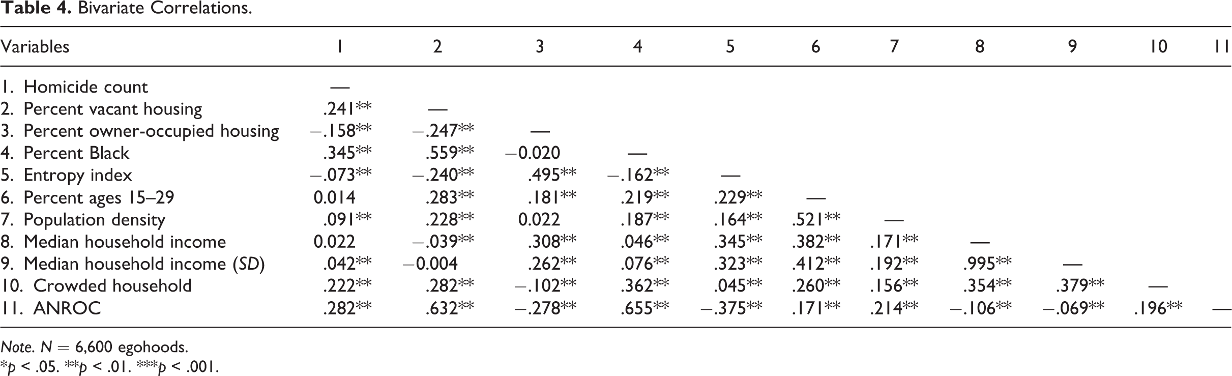
Table 4 presents results of our bivariate correlations. Except for entropy and median household income, all the bivariate associations were consistent with previous research. Specifically, homicides were more likely to occur in neighborhoods that featured greater rates of vacant housing and percent Black, greater population density, more crowded households, and higher values of the ANROC measure. Our entropy measure was negatively associated with homicide, which indicates homicides were less likely to occur in areas of greater segregation. This is a function of the spatial segregation of Baton Rouge, which features an intense north/south racial divide (Cable, 2013), while exploratory spatial data analysis of homicide in Baton Rouge showed that homicides were concentrated in several areas throughout the city. Median household income featured a similar spatial distribution to racial segregation in Baton Rouge, so we believe the reason for the nonsignificant correlation with homicide is similar to that of the negative association with entropy. Inspection of the correlations among the independent variables identified several moderate correlations, but variance inflation factor scores were not determined to be problematic for the regression analyses.

Table 4.

Bivariate Correlations.

Variables	1	2	3	4	5	6	7	8	9	10	11
1. Homicide count	—
2. Percent vacant housing	.241**	—
3. Percent owner-occupied housing	−.158**	−.247**	—
4. Percent Black	.345**	.559**	−0.020	—
5. Entropy index	−.073**	−.240**	.495**	−.162**	—
6. Percent ages 15–29	0.014	.283**	.181**	.219**	.229**	—
7. Population density	.091**	.228**	0.022	.187**	.164**	.521**	—
8. Median household income	0.022	−.039**	.308**	.046**	.345**	.382**	.171**	—
9. Median household income (SD)	.042**	−0.004	.262**	.076**	.323**	.412**	.192**	.995**	—
10. Crowded household	.222**	.282**	−.102**	.362**	.045**	.260**	.156**	.354**	.379**	—
11. ANROC	.282**	.632**	−.278**	.655**	−.375**	.171**	.214**	−.106**	−.069**	.196**	—

Note. N = 6,600 egohoods.

*p < .05. **p < .01. ***p < .001.

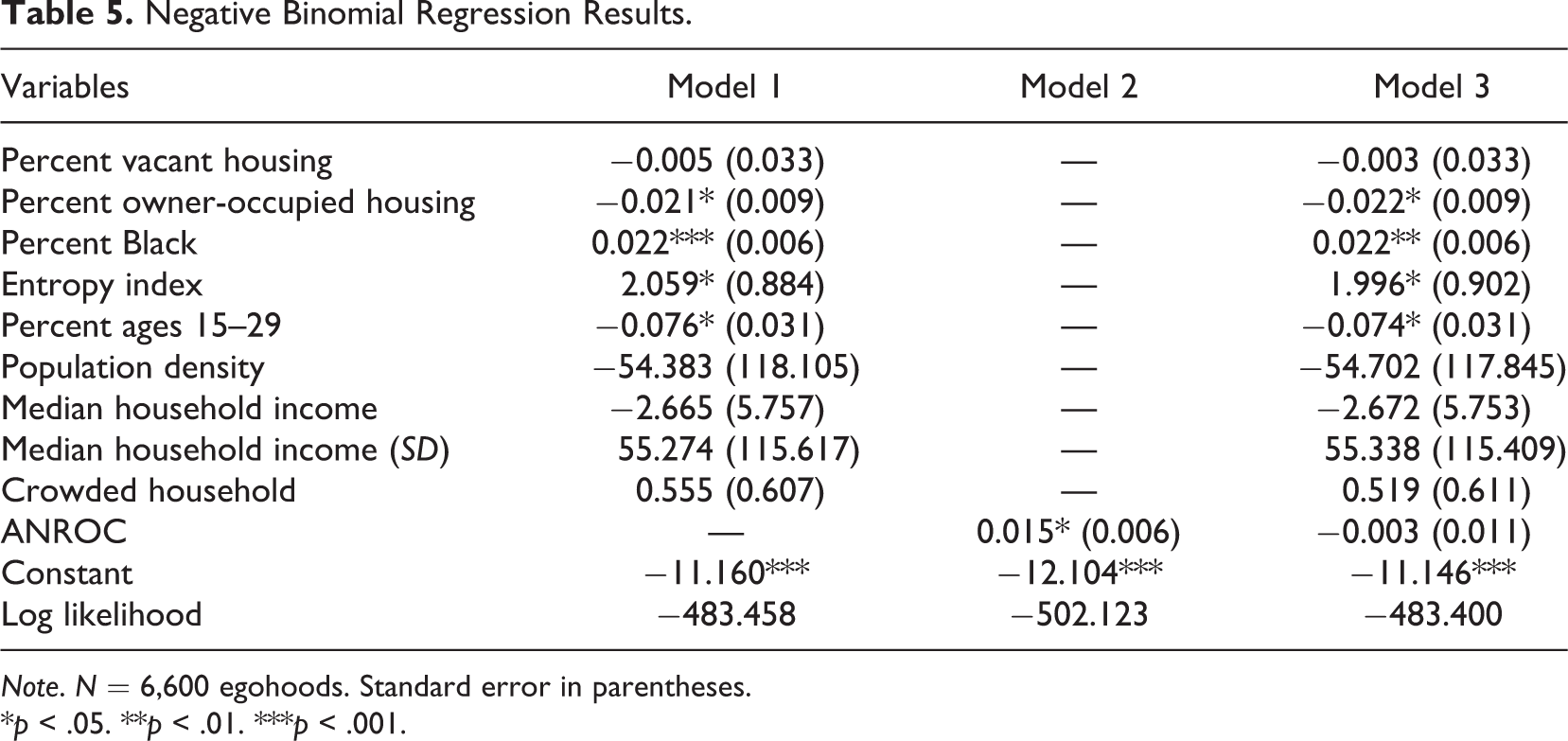
Results of our multivariate regression analyses are presented in Table 5. Neighborhood population was used as an exposure term in all models. Model 1 regressed the number of homicides per egohood on the census-based characteristics of neighborhood disadvantage. As anticipated given prior research and the bivariate correlations, homicide counts were significantly higher in neighborhoods that featured larger black populations (β = 0.022***) and lower rates of homeownership (β = −0.021*).

Table 5.

Negative Binomial Regression Results.

Variables	Model 1	Model 2	Model 3
Percent vacant housing	−0.005 (0.033)	—	−0.003 (0.033)
Percent owner-occupied housing	−0.021* (0.009)	—	−0.022* (0.009)
Percent Black	0.022*** (0.006)	—	0.022** (0.006)
Entropy index	2.059* (0.884)	—	1.996* (0.902)
Percent ages 15–29	−0.076* (0.031)	—	−0.074* (0.031)
Population density	−54.383 (118.105)	—	−54.702 (117.845)
Median household income	−2.665 (5.757)	—	−2.672 (5.753)
Median household income (SD)	55.274 (115.617)	—	55.338 (115.409)
Crowded household	0.555 (0.607)	—	0.519 (0.611)
ANROC	—	0.015* (0.006)	−0.003 (0.011)
Constant	−11.160***	−12.104***	−11.146***
Log likelihood	−483.458	−502.123	−483.400

Note. N = 6,600 egohoods. Standard error in parentheses.

*p < .05. **p < .01. ***p < .001.

The direction of the association of homicide counts with entropy was negative in the bivariate results but was positive in the regression results (β = 2.059*) controlling for other neighborhood characteristics. This is a function of the spatial distribution of the racial groups and measures of neighborhood disadvantage. Specifically, neighborhoods in North Baton Rouge were more likely to feature higher rates of Black residents, vacant housing, crowded housing, and lower median household incomes.

We start to examine the relationship of homicide with the ANROC measure in Model 2. The results indicate that homicides were more likely to occur in neighborhoods that featured higher ANROC scores (β = 0.015*). This finding is consistent with prior research highlighting the important relationship between the built environment, physical disorder (e.g., blighted properties) and neighborhood crime (Drawve, 2016; Thomas & Drawve, 2018; Valasik et al., 2018).

Model 3 assessed the relationship of homicide with the census-based of neighborhood structure and the ANROC. Similar to results of Model 1, we find homicides were more likely occur in neighborhoods that featured higher rates of Black residents (β = 0.022**) and greater segregation (β = 1.996*) controlling for other neighborhood characteristics. Results also indicate homicides were less likely to occur in neighborhoods that featured greater rates of owner-occupied housing units (β = −0.022*) and that featured greater rates of residents in the age range of 15 and 29 (β = −0.074*) controlling for other neighborhood characteristics. In contrast with Model 2, however, the coefficient for ANROC was not significant. This suggests that any influence of neighborhood environmental characteristics on homicide operated through social characteristics of neighborhood populations as predicted by the social disorganization framework (Sampson, 2012; Sampson & Raudenbush, 1999).

Discussion

Efforts to combat crime through remediation of the built environment have a long history and policy makers have increasingly drawn upon these strategies as a mechanism to inhibit crime in disadvantaged communities (Branas et al., 2018; MacDonald et al., 2019; Wilcox et al., 2018). Yet questions remain about whether the social structural characteristics of a neighborhood or the built environment better predict crime. The current study built upon Valasik and colleagues (2019) findings by assessing the relationship of neighborhood homicide levels with social structural neighborhood characteristics through an ANROC measure created with RTM. Our results are consistent with Valasik and colleagues (2019) as they indicate the ANROC measure was a significant predictor of homicide in Baton Rouge neighborhoods. We also found that the inclusion of several social structural characteristics of neighborhoods were more important (see Model 3). In addition to highlighting the greater importance of social structural characteristics of neighborhoods for crime, the current study contributed to research on the neighborhood correlates of crime by operationalizing neighborhoods using Hipp and Boessen’s (2013) egohood approach.

The broken windows thesis has received a great deal of attention among researchers and policy makers, but empirical assessments provided little support for claims that crime was directly associated with neighborhood’s level of physical disorder (Gau & Pratt, 2008; Gault & Silver, 2008; Markowitz et al., 2001; Sampson & Raudenbush, 1999; Wilcox et al., 2018). The lack of a direct relationship of disorder with crime was further supported in the current study. Specifically, we found that the ANROC, the compounding of significant environment risk factors (i.e., the concentration of blighted properties and the proximity to a convenience stores) was associated with the prevalence of neighborhood homicides until social structural characteristics were controlled. This finding diverges slightly from Drawve’s (2016) examination of violent crime rates (e.g., homicide, aggravated assault and robbery) in Little Rock, AR, which indicated that controlling for the social structural characteristics of a neighborhood attenuates the ANROC measure but still significantly influences patterns of neighborhood violence. This disparity among mid-sized cities located in the same regional area showcases how the settings of urban areas are unique across jurisdictions. A turn of the “crime kaleidoscope” reveals a distinct combination of environment risk factors and local contexts that are predictive of violence to a particular jurisdiction (see Barnum et al., 2017). As such, the generalizability of such findings about urban areas may be less practical than prior research has suggested (Connealy, 2019).

Additionally, our results suggest the interrelationship of social (i.e., concentrated disadvantage, residential instability) and physical correlates of violent crime are empirically distinct features (Drawve et al., 2018). The divergence of our findings from those reported by Drawve and colleagues (2018) may be due to different areal units (i.e., egohoods compared to census tracts), divergent social structural measures, and/ or the significance of spatial risk factors in the present study’s RTM that differ. Like Gault and Silver (2008), we propose that the current findings do not suggest that features of the physical environment (i.e., concentration of blighted properties and the proximity to a convenience store) were unimportant in influencing lethal violence in a neighborhood. Instead, we suggest the relationship of physical disorder with crime is more complex than was often discussed in the criminological literature. Beyond simply replicating the current study in other municipalities or by examining other types of crime, future research could explore this complex relationship between physical disorder, as measured through ANROC, and the social structural environment of a community through structural equation modeling which is better able to account for measurement error in the predictor variables (see Bollen, 2002).

Another contribution of the current study was the operationalization of neighborhoods using the egohood approach (Hipp & Boessen, 2013; Kim & Hipp, 2019). Drawve and colleagues (2018, p. 18) suggest that the combination of ANROC and egohoods could provide a more nuanced approach to understanding the relationship between the “environmental backcloth” of a neighborhood and crime. Much of the research on neighborhood correlates of crime analyzes variation in tract level measures of crime despite widely discussed limitations (Gerell, 2018; Hipp, 2007; Hipp & Bates, 2018; Tita & Radil, 2010; Vogel, 2016). The development and use of egohoods as a units of analysis represent one possible strategy for addressing the critique that tracts do not match well with the neighborhood areas or activity spaces recognized by residents (see Hipp & Bates, 2018; Hipp, Williams, & Boessen, 2018). A challenge to using egohoods, however, is that they are best created using data from the smallest units of analysis possible. Like Hipp and Boessen (2013), we used a combination of census blocks and census block groups because only a limited number of census measures were available at the block level.

It is important to recognize several limitations of our study. First, our study focused on a single medium-sized city in the Southern United States, and our analyses were limited to neighborhood variation in homicide. Thus, findings from the current study may only be generalizable to jurisdictions comparable in size to Baton Rouge. Second, egohoods were better conceptual neighborhood units than the commonly used census tracts, but we did not fully engage with the MAUP. Results of sensitivity analyses conducted with block groups reported similar findings. That is, the block group ANROC measure was significantly associated with homicide when controls were not included and not significant when controls were included. Barnum and colleagues (2017) contend that the settings for different jurisdictions are unique and that a turn of the crime kaleidoscope assembles a distinct combination of situational contexts and spatial risk factors for each RTM analysis, producing a different mixture of environmental characteristics that successfully forecast types of crimes (see also Connealy, 2019). As for the creation of the ANROC measure, the environmental risk factors included in the current study’s RTM analysis were guided by personal knowledge of Baton Rouge (see Valasik et al., 2018) and the extant criminological literature to formulate an exhaustive list. It remains possible that important environmental risk factors were not included in the current study and our analyses experience omitted variable bias.

While the current study builds on the growing RTM and egohoods’ literatures contributing to advancements in place-based methods, there are also important policy implications from our findings. Principally, it appears that strategies aimed at reducing crime and violence by solely dealing with the built environment, such as crime prevention through environmental design (CPTED; MacDonald, 2015), blight remediation (Branas et al., 2018; Kondo et al., 2018; MacDonald et al., 2019), or gentrification (Barton, 2016; Barton et al., 2019; Papachristos et al., 2011) in Baton Rouge or analogous municipalities may only provide a temporary downturn in lethal violence. Instead, given the stronger relationship between the social structural characteristics of neighborhoods with homicide to achieve a more long-term goal of eliminating lethal violence, it is necessary to address what Currie (2013) calls the “root causes” of crime: poverty, social exclusion, marginalizing youth, and lack of opportunity. The current study’s findings would support Currie’s proposition.

Conclusion

Despite the limited support for the broken windows thesis, city officials in municipalities across the country have continued to look to neighborhood revitalization strategies such as gentrification and blight reduction to address neighborhood crime and violence problems (Barton, 2016; Barton et al., 2019; Branas et al., 2018; Kondo et al., 2018; Wilcox et al., 2018). The results of the current study indicate that while the physical landscape of a neighborhood was a strong predictor of violent crime, the social structural features of neighborhoods appear to be more important, particularly over the long term. This is not to say efforts to improve the physical environment (e.g., blight reduction, CPTED) of a neighborhood are unimportant, as prior research indicates that neighborhood upkeep does matter (Branas et al., 2018; Kondo et al., 2018; MacDonald et al., 2019). Instead, we suggest the relationship of physical disorder and homicide may be indirect (see Gault and Silver, 2008) and strategies like blight abatement/ remediation may have other important implications for neighborhoods such as improved health and reductions in fear of crime (Branas et al., 2018; Kondo et al., 2018; MacDonald et al., 2019).

Given limitations of the current study and improvements in the ANROC as a measure of an area’s spatial vulnerability and exposure to criminal events (i.e., homicide), we encourage future research to continue investigating the relationship between physical disorder, the social structural environment, and crime in other municipalities using other types of violent crime (e.g., robbery, aggravated assault) as the dependent variable. Additionally, studies should examine neighborhood’s ANROC and social structural environment over time to examine how these relationships vary with violent crime (e.g., homicide) in response to changes in an area’s relative risk (e.g., blight remediation).

Advancing research on where crime occurs requires engagement with two issues. First, more information about incidents of crime for areas along the urbanization spectrum needs to become available. Neighborhood research on crime has long suffered from urban bias with very little research conducted about crime in suburban or rural areas due to data limitations. The release of the National Neighborhood Crime Study data represents a strong first step (Peterson & Krivo, 2010b). Additionally, cities across the country have increasingly released publicly accessible data portals from which information about crime incidents can be downloaded. Second, researchers should provide greater access to the programming required to replicate analyses. For example, the current study was able to create egohoods because of code that was publicly available on Irvine Laboratory for the Study of Space and Crime’s website (Irvine Laboratory for the Study of Space and Crime, 2020). Engagement with these issues will facilitate the development of a more unified body of knowledge about where crimes have occurred in the past and where they ultimately might occur in the future.

Footnotes

Authors’ Note

Michael S. Barton and Matthew A. Valasik shared equal authorship.

Declaration of Conflicting Interests

The authors declared no potential conflicts of interest with respect to the research, authorship, and/or publication of this article.

Funding

The authors received no financial support for the research, authorship, and/or publication of this article.

ORCID iDs

Matthew A. Valasik

Elizabeth Brault

Notes

References

Apparicio

Fournier

É.

Apparicio

(2013). Geo-segregation analyzer: A multiplatform application (Version 1.1). In (SAREL) SAaREL (Ed.). INRS Urbanization Culture Societe.

Barnum

J. D.

Caplan

J. M.

Kennedy

L. W.

Piza

E. L.

(2017). The crime kaleidoscope: A cross-jurisdictional analysis of place features and crime in three urban environments. Applied Geography, 79, 203–211.

Barthelemy

J. J.

Chaney

Maccio

E. M.

Church

W. T.

(2016). Law enforcement perceptions of their relationship with community: Law enforcement surveys and community focus groups. Journal of Human Behavior in the Social Environment, 26, 413–429.

Barton

M. S.

(2016). Gentrification and violent crime in New York City. Crime & Delinquency, 62, 1180–1202.

Barton

M. S.

Valasik

Brault

Tita

(2019). “Gentefication” in the Barrio: Examining the relationship between gentrification and homicide in East Los Angeles. Crime & Delinquency, 66, 1888–1913.

Bernasco

Block

(2011). Robberies in Chicago: A block-level analysis of the influence of crime generators, crime attractors, and offender anchor points. Journal of Research in Crime and Delinquency, 48: 33–57.

Bollen

K. A.

(2002). Latent variables in psychology and the social sciences. Annual Review of Psychology, 53, 605–634.

Braga

A. A.

Papachristos

A. V.

Hureau

D. M.

(2010). The concentration and stability of gun violence at micro places in Boston, 1980–2008. Journal of Quantitative Criminology, 26(1), 33–53.

Braga

A. A.

Welsh

B. C.

Schnell

(2015). Can policing disorder reduce crime? A systematic review and meta-analysis. Journal of Research in Crime and Delinquency, 52, 567–588.

10.

Branas

C. C.

South

Kondo

M. C.

Hohl

B. C.

Bourgois

Wiebe

D. J.

MacDonald

J. M.

(2018). Citywide cluster randomized trial to restore blighted vacant land and its effects on violence, crime, and fear. Proceedings of the National Academy of Sciences, 115, 2946–2951.

11.

Brantingham

P. J.

Brantingham

P. J.

(1981). Environmental criminology. Sage.

12.

Brantingham

P. J.

Brantingham

P. L.

(1984). Patterns in crime. Macmillan.

13.

Brantingham

P. L.

Brantingham

P. J

. (1993). Environment, routine, and situation: Toward a pattern theory of crime. In Ronald V. Clarke and Marcus Felson (Eds.), Routine activity and rational choice: Advances in criminological theory (pp 259–294). Routledge.

14.

Brantingham

P. L.

Brantingham

P. J.

(1995). Criminality of place. European Journal on Criminal Policy and Research, 3, 5–26.

15.

Cable

(2013). The racial dot map. Retrieved March 30, 2019 from https://demographics.coopercenter.org/index.php/racial-dot-map#overview

16.

Caplan

J. M.

Kennedy

L. W.

(2016). Risk terrain modeling: Crime prediction and risk reduction. University of California Press.

17.

Caplan

J. M.

Kennedy

L. W.

Barnum

J. D.

Piza

E. L.

(2013). Risk terrain modeling diagnostics utility user manual (Version 1). Rutgers Center on Public Security, Rutgers, NJ.

18.

Caplan

J. M.

Kennedy

L. W.

Barnum

J. D.

Piza

E. L.

(2017). Crime in context: Utilizing risk terrain modeling and conjunctive analysis of case configurations to explore the dynamics of criminogenic behavior settings. Journal of Contemporary Criminal Justice, 33(2), 133–151.

19.

Caplan

J. M.

Kennedy

L. W.

Miller

(2011). Risk terrain modeling: Brokering criminological theory and GIS methods for crime forecasting. Justice Quarterly, 28(2), 360–381.

20.

Caplan

J. M.

Kennedy

L. W.

Piza

E. L.

(2013). Joint utility of event-dependent and environmental crime analysis techniques for violent crime forecasting. Crime & Delinquency, 59(2), 243–270.

21.

Caplan

J. M.

Marotta

L Piza

W Kennedy

(2014). Spatial risk factors of felonious battery to police officers. Policing: An International Journal of Police Strategies & Management, 37(4), 823–838.

22.

Cohen

L. E.

Felson

(1979). Social change and crime rate trends: A routine activity approach. American Sociological Review, 44, 588–608.

23.

Connealy

N. T.

(2019). Can we trust crime predictors and crime categories? Expansions on the potential problem of generalization. Applied Spatial Analysis and Policy. https://doi.org/10.1007/s12061-019-09323-5

24.

Currie

(2013). Crime and punishment in America (2nd ed.). Picador.

25.

Drawve

, (2016). A metric comparison of predictive hot spot techniques and RTM. Justice Quarterly, 33, 369–397.

26.

Drawve

Grubb

Steinman

Belongie

(2018). Enhancing data-driven law enforcement efforts: Exploring how risk terrain modeling and conjunctive analysis fit in a crime and traffic safety framework. American Journal of Criminal Justice, 44, 106–124.

27.

Drawve

Moak

S. C.

Berthelot

E. R.

(2014). Predictability of gun crimes: A comparison of hot spot and risk terrain modelling techniques. Policing and Society, 26(3), 312–331.

28.

Dugato

(2013). Assessing the validity of risk terrain modeling in a European City: Preventing robberies in the city of Milan. Crime Mapping, 5(1), 63–89.

29.

Dugato

Calderoni

Berlusconi

(2020). Forecasting organized crime homicides: Risk terrain modeling of camorra violence in Naples, Italy. Journal of Interpersonal Violence, 35(19-20), 4013–4039.

30.

Federal Bureau of Investigation, U.S. Department of Justice. Office of Justice Programs. (2016). Uniform crime reporting program data. Inter-university Consortium for political and social research. https://www.icpsr.umich.edu/web/NACJD/studies/36789

31.

Felson

(1987). Routine activities and crime prevention in the developing metropolis. Criminology, 25, 911–932.

32.

Ferguson

A. G.

(2019). The rise of big data policing: Surveillance, race, and the future of law enforcement. NYU Press.

33.

Garnier

Caplan

J. M.

Kennedy

L. W.

(2018). Predicting dynamical crime distribution from environmental and social influences. Frontiers in Applied Mathematics and Statistics, 4, 1–10.

34.

Gau

J. M.

Pratt

T. C.

(2008). Broken windows or window dressing? Citizens’ (in)ability to tell the difference between disorder and crime. Criminology & Public Policy, 7, 163–194.

35.

Gault

Silver

(2008). Spuriousness or mediation? Broken windows according to Sampson and Raudenbush (1999). Journal of Criminal Justice, 36, 240–243.

36.

Gerell

(2018). Bus stops and violence, are risky places really risky? European Journal on Criminal Policy and Research, 24, 351–371. https://doi.org/10.1007/s10610-018-9382-5

37.

Giménez-Santana

Caplan

J. M.

Drawve

(2018). Risk terrain modeling and socio-economic stratification: Identifying risky places for violent crime victimization in Bogotá, Colombia. European Journal on Criminal Policy and Research, 24, 417–431. https://doi.org/10.1007/s10610-018-9374-5

38.

Heffner

(2013). Statistics of the RTMDx utility (pp. 26–34). In Caplan

Kennedy

Piza

(Eds.), Risk terrain modeling diagnostics utility user manual (Version 1). Rutgers Center on Public Security.

39.

Hipp

J. R.

(2007). Income inequality, race, and place: Does the distribution of race and class within neighborhoods affect crime rates? Criminology, 45, 665–697.

40.

Hipp

J. R.

Bates

C. J.

(2018). Egohoods: Capturing change in spatial crime patterns. In Bruinsma

G. J. N.

Johson

S. D.

, (Eds.), The Oxford handbook of environmental criminology. Oxford University Press.

41.

Hipp

J. R.

Boessen

(2013). Egohoods as waves washing across the city: A new measure of “neighborhoods.” Criminology, 51, 287–327.

42.

Hipp

J. R.

Williams

S. A

. (2020). Advances in spatial criminology: The spatial scale of crime. Annual Review of Criminology, 3, 75–95. https://doi.org/10.1146/annurev-criminol-011419-041423.

43.

Hipp

J. R.

Williams

S. A.

Boessen

(2018). Disagreement in assessing neighboring and collective efficacy: The role of social distance. Socius: Sociological Research for a Dynamic World, 4(3), 1–16.

44.

Irvine Laboratory for the Study of Space and Crime (2020). Egohoods. Retrieved September 28, 2020, from https://ilssc.soceco.uci.edu/applications/egohood/

45.

Jacobs

(1961). The death and life of great American cities. Random House.

46.

Johnson

. (2013). Chicago not actually “murder capital” of, well, anything. Retrieved May 25, 2018, from http://chicago.cbslocal.com/2013/09/26/chicago-not-actually-murdercapital-of-well-anything/

47.

Kelling

G. L.

Coles

C. M.

(1996). Fixing broken windows: Restoring order and reducing crime in our communities. Martin Kessler Books.

48.

Kennedy

L. W.

Caplan

J. M.

Piza

E. L.

Buccine-Schraeder

(2016). Vulnerability and exposure to crime: Applying risk terrain modeling to the study of assault in Chicago. Applied Spatial Analysis and Policy, 9(4), 529–548.

49.

Kennedy

L. W.

Caplan

J. M.

Piza

E. L

. (2011). Risk clusters, hotspots, and spatial intelligence: Risk terrain modeling as an algorithm for police resource allocation strategies. Journal of Quantitative Criminology, 27, 339–362.

50.

Kim

Y. A.

(2016). Examining the relationship between the structural characteristics of place and crime by imputing census block data in street segments: Is the pain worth the gain? Journal of Quantitative Criminology, 34, 67–110.

51.

Kim

Y. A.

Hipp

J. R.

(2017). Physical boundaries and city boundaries: Consequences for crime patterns on street segments? Crime & Delinquency, 64, 227–254.

52.

Kim

Y-A.

Hipp

J. R.

(2019). Street egohood: An alternative perspective for measuring neighborhood and spatial patterns of crime. Journal of Quantitative Criminology. https://doi.org/10.1007/s10940-019-09410-3

53.

Kirk

D. S.

Laub

J. H.

(2010). Neighborhood change and crime in the modern metropolis. Crime and Justice, 39(1), 441–502.

54.

Kocher

Leitner

(2015). Forecasting of crime events applying risk terrain modeling. Gi_Forum, 1, 30–40.

55.

Kondo

M. C.

Morrison

Jacoby

S. F.

Elliott

Poche

Theall

K. P.

Branas

C. C.

(2018). Blight abatement of vacant land and crime in New Orleans. Public Health Reports, 133, 650–657.

56.

Koss

K. K.

(2015). Leveraging predictive policing algorithms to restore fourth amendment protections in high-crime areas in a post-Wardlow world. Chi.-Kent Law Review, 90, 301.

57.

Kubrin

C. E.

Hipp

J. R.

(2016). Do fringe banks Create fringe neighborhoods? Examining the spatial relationship between fringe banking and neighborhood crime rates. Justice Quarterly, 33, 755–784. https://doi.org/10.1080/07418825.2014.959036

58.

Land

K. C.

McCall

P. L.

Cohen

L. E.

(1990). Structural covariates of homicide rates: Are there any invariances across time and social space? American Journal of Sociology, 95(4), 922–963.

59.

Lane

. (2017). Louisiana’s murder rate again leads U.S.: See how other states compare. In The Times Picayune. Retrieved March 15, 2018, from http://www.nola.com/crime/index.ssf/2017/09/louisiana_murder_rate_fbi_crim.html

60.

Lersch

K. M.

(2017). Risky places: An analysis of carjackings in Detroit. Journal of Criminal Justice, 52, 34–40. http://doi.org/10.1016/j.jcrimjus.2017.07.011

61.

Light

M. T.

Thomas

J. T.

(2019). Segregation and violence reconsidered: Do whites benefit from residential segregation? American Sociological Review, 84, 690–725.

62.

MacDonald

(2015). Community design and crime: the impact of housing and the built environment. Crime Justice, 44, 333–557.

63.

MacDonald

Branas

Stokes

(2019). Changing places: The science and art of new urban planning. Princeton University Press.

64.

MacDonald

J. M.

Stokes

R. J.

(2020). Gentrification, land use, and crime. Annual Review of Criminology, 3(1), 121–138. http://doi.org/10.1146/annurev-criminol-011419-041505

65.

Manson

Schroeder

Van Riper

Ruggles

. (2019) IPUMS National Historical Geographic Information System: Version 14.0 [Database]. IPUMS. http://doi.org/10.18128/D050.V14.0

66.

Markowitz

F. E.

Bellair

P. E.

Liska

A. E.

Liu

(2001). Extending social disorganization theory: Modeling the relationships between cohesion, disorder, and fear. Criminology, 39, 293–320.

67.

McCall

P. L.

Land

K. C.

Parker

K. F.

(2010). An empirical assessment of what we know about structural covariates of homicide rates: A return to a classic 20 years later. Homicide Studies, 14(3), 219–243.

68.

Mears

D. P.

Bhati

A. S.

(2006). No community is an island: The effects of resource deprivation on urban violence in spatially and socially proximate communities. Criminology, 44(3), 506.

69.

Papachristos

A. V.

Smith

C. M.

Scherer

M. L.

Fugiero

M. A.

(2011). More coffee, less crime: The relationship between gentrification and neighborhood crime rates in Chicago, 1991 to 2005. City & Community, 10, 215–240.

70.

Peterson

R. D.

Krivo

L. J.

(2010a). Divergent social worlds: Neighborhood crime and the racial-spatial divide. Russell Sage Foundation.

71.

Peterson

R. D.

Krivo

L. J

. (2010b). National Neighborhood Crime Study (NNCS), 2000: Inter-university Consortium for political and social research. https://doi.org/10.3886/ICPSR27501.v1

72.

Piza

E. L.

Feng

Kennedy

L. W.

Caplan

J. M.

(2016). Place-based correlates of motor vehicle theft and recovery: Measuring spatial influence across neighborhood context. Urban Studies, 54, 2998–3021.

73.

Priola

Kron

. (2018). The city of Baton Rouge—Parish of East Baton Rouge GIS. Retrieved May 25, 2018, from data.br.gov

74.

Rosenfeld

Bray

T. M.

Egley

(1999). Facilitating violence: A comparison of gang-motivated, gang-affiliated, and nongang youth homicides. Journal of Quantitative Criminology, 15, 495–516.

75.

Rosenfeld

Fornango

Rengifo

A. F.

(2007). The impact of order-maintenance policing on New York City homicide and robbery rates: 1988-2001. Criminology, 45, 355–384.

76.

Rountree

P. W.

Land

K. C.

Miethe

T. D.

(1994). Macro-micro integration in the study of victimization: A hierarchical logistic regression model analysis across Seattle neighborhoods. Criminology, 32, 387–414.

77.

Sampson

R. J.

(2012). Great American city: Chicago and the enduring neighborhood effect. The University of Chicago Press.

78.

Sampson

R. J.

Raudenbush

S. W.

(1999). Systematic social observation of public spaces: A new look at disorder in urban neighborhoods. The American Journal of Sociology, 105, 603–651.

79.

Shaw

C. R.

McKay

H. D.

(1969). Juvenile delinquency and urban areas (3rd ed.). The University of Chicago Press. (Original work published 1942)

80.

Sheppard

Grant

Rowe

Jacobs

(2000). Fighting juvenile gun violence. Juvenile Justice Bulletin (pp. 182–679). Office of Juvenile Justice, Delinquency, and Programs.

81.

Skogan

W. G.

(1990). Disorder and decline: Crime and the spiral of decay in American neighborhoods. The Free Press.

82.

Steinman

Drawve

Datta

Harris

C. T.

Thomas

S. A.

(2020). Risky business: Examining the 80-20 rule in relation to a RTM framework. Criminal Justice Review. https://doi.org/10.1177/0734016820938859

83.

Suttles

G. D.

(1972). The social construction of communities. University of Chicago Press.

84.

Taylor

R. B.

(2001). Breaking away from broken windows: Baltimore neighborhoods and the nationwide fight against crime, grime, fear, and decline. Westview Press.

85.

Thomas

(2017). Baton rouge lands in top 25 on America’s 25 murder capitals list. WAFB News. Retrieved March 15, 2018 from http://www.wafb.com/story/36853780/batonrouge-lands-in-top-25-on-americas-25-murder-capitals-list

86.

Thomas

S. A.

Drawve

(2018). Examining interactive effects of characteristics of the social and physical environment on aggravated assault.” Journal of Crime Justice, 57, 89–98.

87.

Tita

G. E.

Greenbaum

R. T.

(2009). Crime, neighborhoods, and units of analysis: Putting space in its place. In: Weisburd

Bernasco

Bruinsma

(Eds.), Putting crime in its place (pp. 145–170). Springer.

88.

Tita

G. E.

Griffiths

(2005). Traveling to violence: The case for a mobility-based spatial typology of homicide. Journal of Research in Crime and Delinquency, 42, 275–308.

89.

Tita

G. E.

Radil

S. M.

(2010). Making space for theory: The challenges of theorizing space and place for spatial analysis in criminology. Journal of Quantitative Criminology, 26(4), 467–479.

90.

U.S. Census Bureau. (2017). Population estimates: Baton Rouge city, Louisiana. Population Estimates. Retrieved March 15, 2018, from www.census.gov/quickfacts/fact/table/batonrougecitylouisiana/PST045217

91.

Valasik

(2018). Gang violence predictability: Using risk terrain modeling to study gang homicides and gang assaults in East Los Angeles. Journal of Crime Justice, 58, 10–21.

92.

Valasik

Barton

M. S.

Reid

S. E.

Tita

G. E.

(2017). Barriocide: Investigating the temporal and spatial influence of neighborhood structural characteristics on gang and non-gang homicides in East Los Angeles.” Homicide Studies, 21(4), 287–311. https://doi.org/10.1177/1088767917726807

93.

Valasik

Brault

E. E.

Martinez

S. M.

(2019). Forecasting homicide in the red stick: Risk terrain modeling and the spatial influence of urban blight on lethal violence in Baton Rouge, Louisiana. Social Science Research, 80, 186–201.

94.

Vogel

(2016). The modifiable areal unit problem in person-context research. Journal of Research in Crime and Delinquency, 53, 112–135.

95.

Weatherburn

Lind

(1999). Hotbeds of crime? Crime and public housing in urban Sydney. Crime Delinquency, 45, 256–271.

96.

Wilcox

Cullen

F. T

Feldmeyer

(2018). Communities and crime: An enduring American challenge. Temple University Press.

97.

Wilson

J. Q.

Kelling

G. L.

(1982, March). Broken windows: The police and neighborhood safety. The Atlantic Monthly. 29–37.