
Abstract
Steel is an ideal recycling material as it can be recycled almost indefinitely, and steel recycling is a lot more energy-efficient than iron ore steel production. Steel making with usage of steel scrap in electric arc furnaces is heavily influenced by contaminants in the scrap, including non-ferrous metals, stones, or plastic. To produce high-quality steel, it is important to know what contaminants are part of the scrap to adapt the recycling process accordingly. This work presents a three-part processing pipeline to determine the scrap composition and optimise the recycling process parameters. The first part is hyperspectral imaging, recording images with 437 spectral bands in the short-wave infrared range. Next, deep learning-based image recognition, with multilayer perceptron, 2D and 3D convolutional neural networks (CNNs) have been compared. The 3D-CNN showed the best performance in detecting the 14 material classes in the scrap samples. Finally, a mixed integer optimisation is used to select the best scrap mix for the steel classes that are to be produced. The evaluation shows an accuracy of about 76% in detecting the 14 material classes correctly, with a higher accuracy for the steel class. The detected non-ferrous materials determine the scrap class which is input for the optimisation with its constraints that each scrap class has a minimum consumption to prevent storage overflows, and as little energy and additives as possible should be used.
Keywords
Introduction
Steel recycling is an important aspect in decreasing CO2 emissions and the usage of landfill capacity. Due to its material properties, steel can be recycled almost indefinitely and therefore provides a good base for novel recycling processes. However, the demand for steel is high, and forecasts reveal that the crude steel demand will be 30% higher in 2050 than it is today (Mission Possible Partnership [MPP], 2021; Morfeldt et al., 2015). Due to the innovations in refuse sorting and scrap management, an increasing availability of steel scrap is also expected, meaning that the contribution of scrap to the total steel charge will likely grow to 40% in 2050 from 30% today (MPP, 2021). Hence, steel works require ways to incorporate more and more scrap in their production processes, so that the increased scrap input increases the steel recycling rates, therefore reducing the CO2 emissions. At the same time, the requirements of the desired steel qualities need to be fulfilled, and the general movement towards the increased use of electric arc furnaces (EAFs) supported without increasing the production cost (Harvey, 2021). To overcome these challenges, the steel recycling industry is looking towards technologies that have proven themselves in the recycling of other materials (Colla et al., 2020).
One key technology is the characterisation of scrap particles in terms of their composition, made of ferrous and non-ferrous metals, plastics, and other undesired fractions. Knowing the scrap composition allows to react, adapt, and optimise the steel recycling process with respect to the ever-changing compositions of steel scrap. This work presents a pipeline consisting of hyperspectral image capturing, image recognition, and scrap composition optimisation. The pipeline was implemented in laboratory conditions and used scrap samples provided by Austrian steel recycling works. The methods and the presented results show how a hyperspectral imaging system can be designed and used to detect the material compositions with deep learning models. Three different models for the image recognitions are trained, and the best model is evaluated in detail. The results of the image recognition are the input for the optimisation. With this input, the optimisation calculates the best possible scrap composition for an EAF given the available scrap, the desired steel quality to be produced, and the boundary conditions of the process, for instance the energy need or available scrap amounts.
The next section gives a brief overview of related work. This is followed by a description of the implementation in section ‘Method and implementation’ and the results in section ‘Results and discussion’. This publication ends with a discussion of the results and an outlook of future work in section ‘Conclusion and outlook’.
Related work
Steel production is shifting towards EAF steel production motivated by a reduction of fossil fuel and energy consumption, thus resulting in reduced CO2 emissions compared to blast furnace-basic oxygen furnace production. EAFs are especially beneficial when a 100% scrap-rate is achieved, and no direct reduction plant is installed upstream of the EAF (Perpiñán et al., 2023). To satisfy the global steel demand, an increasing share of post-consumer scrap is processed (Morfeldt et al., 2015). However, high-grade steel suffers from tramp elements such as copper, tin, chromium, nickel, or molybdenum as well as non-metal impurities such as stone or plastics in post-consumer scrap. Therefore, the steel industry is looking for new solutions increasing the use of low-quality scrap by detecting non-ferrous scrap fractions (Brooks et al., 2019).
A vast array of techniques for detecting the composition of scrap are available: for instance, spectroscopic methods, covering a wide range of technologies including hyperspectral imaging, X-ray-, plasma-, and neutron-based detection methods (Brooks et al., 2019). Although hyperspectral imaging only shows very limited ability to detect beneath surface coatings, it has the benefits of low cost, safe operation, and capabilities to capture whole areas. Hyperspectral imaging primarily captures the near-infrared (NIR), short-wave infrared (SWIR), or mid-wave infrared (MWIR) light spectrum ranges, often combined with the visible red-, green-, and blue (RGB) spectrum. Current NIR and SWIR systems are already deployed industrially, whereas MWIR technology continues to advance but remains relatively costly. Hyperspectral imaging is already utilised in various applications within the circular economy (Menezes et al., 2024).
Such images are input for the machine learning (ML) step classifying the scrap particles. Deep learning techniques are increasingly adopted for hyperspectral image segmentation due to their ability to handle high-dimensional data (Paoletti et al., 2019; Signoroni et al., 2019). Early methods often employed feedforward neural networks or multilayer perceptrons (MLPs), which treat each pixel’s spectral signature as an input vector mapped directly to a class label (Benediktsson et al., 1995). Although MLPs capture non-linear relationships in the spectral domain, ignoring spatial context can limit performance. Consequently, many approaches now integrate spatial information via patch-based inputs or dimensionality reduction, aiming to counter the ‘curse of dimensionality’ inherent in hyperspectral data (Ahmad et al., 2025). Convolutional neural networks (CNNs) have become the predominant choice for hyperspectral segmentation, with 2D or 3D convolutions applied to spatial–spectral cubes to learn local features that differentiate materials with similar reflectance signatures (Chen et al., 2016; Zhao and Du, 2016). Three-dimensional CNNs often capture spectral continuity more effectively but can introduce higher computational loads and potential overfitting risks. Recurrent neural networks, incorporating Long Short-Term Memory (LSTM) or Gated Recurrent Units (GRUs), frame each pixel’s spectral response as sequential data, enabling the modelling of inter-band dependencies (Liu et al., 2017). More recently, transformer-based architectures have shown promise in capturing global context across entire hyperspectral cubes, although they generally require large datasets to mitigate overfitting (Hong et al., 2021).
Multiple works have been published that use deep learning-based hyperspectral segmentation in recycling. Singh et al. (2023) applied hyperspectral imaging and an artificial neural network to classify post-consumer thermoplastics, whereas Picón et al. (2025) investigated segmentation of metals using 1D and 2D-CNNs, demonstrating that full-spectrum data outperforms RGB inputs. The results of the scrap particle classification are the input to improve the steel melting in the EAF. Improvements can reach from detection and separation of unwanted scrap particles (Smirnov and Trifonov, 2021; SORMEN, 2024) to digitalisation of the steel recycling process (Colla et al., 2020). Schäfer et al. (2023) published a multimodal dataset of RGB images captured with smartphone and drone cameras, categorised into standard European scrap classes. Similarly, Xu et al. (2023) also employed traditional RGB images taken during truck unloading in their deep learning framework for multi-category steel scrap classification. Metal recycling facilities utilise hyperspectral segmentation to distinguish alloys, maximising resource recovery and minimising waste (Picón et al., 2025). Optimisation applications are prominent users of such classifications, due to the immediate benefits of improving energy efficiency and reducing costs (Lee et al., 2023; Riesbeck et al., 2011).
Method and implementation
For the project at hand, a processing pipeline with three stages was designed where the first stage is the hyperspectral image capturing, followed by the image recognition and the optimisation of the scrap composition. The experiments were carried out in laboratory conditions with scrap samples provided by Austrian steel recycling companies. The dataset is available in a publicly accessible repository (Jaschik and Jernej, 2025) holding a total 170 images collected in 4 batches. The dataset consists of the hyperspectral images with 437 channels in the spectral range from 948 to 1692 nm and the associated material labels describing the unsorted scrap samples with foreign and contaminating substances. The scrap samples of the dataset were selected, sorted, and classified into desired materials as well as foreign and contaminating materials by experts from the metal manufacturing industry. In the hyperspectral recordings, the wavelengths at the beginning and end of the spectrum were trimmed, since this data lies in the fringe area of the sensor’s sensitivity and is very noisy. This results in more stable signals, saves storage space and in a reduction from 512 down to 437 channels.
The hyperspectral laboratory equipment is shown in Figure 1. The hyperspectral imaging systems operates in the SWIR (up to 2500 nm) and the MWIR (up to 5500 nm, going beyond the typical MWIR of 5000 nm). Due to high cost and low speed, the MWIR camera is not suitable for use in industrial environments in its currently available form, but the SWIR camera is fast enough. Hence, only the SWIR channels are used in the image recognition. The image capturing equipment also includes a 3D laser triangulation camera, which helps to orthorectify the recorded images in relation to each other. All systems are installed above a conveyor belt for continuous transport. During recording, the scrap particles were placed separately to facilitate annotation and to enable and verify AI-assisted counting of the shredder particles.
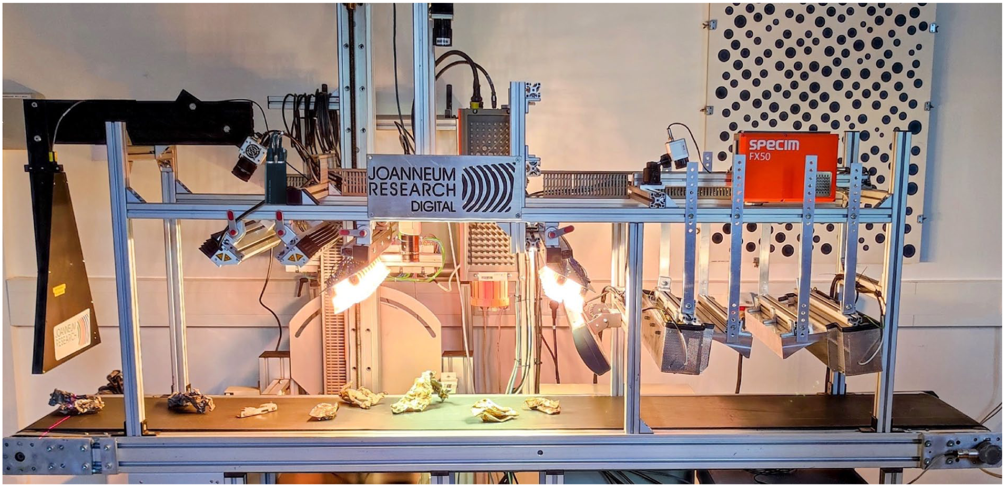
Hyperspectral image capturing system consisting of cameras, lighting, and the conveyor belt moving the scrap particles.
For illumination in the visible spectrum, a specialised LED lighting system for the camera covering RGB and NIR spectrum is used. Lighting for the SWIR range is done by a hybrid setup combining halogen lamps, providing a continuous spectrum up to 2100 nm, and radiant heaters to achieve optimised lighting conditions. However, industrial applications already utilise LED-based illumination systems covering wavelengths up to 1700 nm. For MWIR illumination, a custom-designed heating source featuring a quarter-elliptical radiator was developed.
The hyperspectral image covers the light spectrum from 948 to 1692 nm split into 512 spectral bands, of which 437 are usable. From these hyperspectral images, a unique spectral fingerprint for each material is derived. However, the direct analysis of the raw hyperspectral images is impractical due to the extensive number of spectral bands involved, but these are an ideal input for the image classification. An example of the hyperspectral images is shown in Figure 2 together with the RGB representation. It is harder for the human eye to distinguish the materials in the spectrum of the visible light (Figure 2, left upper image) than by selecting three channels out of the hyperspectral images and displaying them in the RGB spectrum (Figure 2, left lower image). The full hyperspectral signature (Figure 2, right image) shows the different spectral properties.

Hyperspectral images of various materials. Left upper image: RGB image; left lower image: SWIR image with three selected wavelengths represented in RGB spectrum; right image: full hyperspectral information per material.
Three neural network architectures that capture progressively richer spatial–spectral information in hyperspectral images were investigated for the classification of materials. The first model uses an MLP that processes each pixel independently using only its spectral signature. This serves as a baseline to demonstrate how well the other more sophisticated models can improve performance upon a simple approach. The second model is a 2D-CNN taking small image patches as input and predicting the class of the centre pixel. Due to the convolutional filters incorporating information across neighbouring pixels, the model can learn to apply smoothing in a local region, thus making it more robust to measurement noise. Additionally, providing spatial information allows local texture to be incorporated into the prediction. Finally, 3D-CNN was implemented that convolves over both the spectral and spatial dimensions. Unlike 2D kernels, which process the spatial domain for each spectral channel separately, 3D kernels convolve simultaneously over both the spatial and spectral axes. This allows the 3D-CNNs to capture spectral correlations better, resulting in improved classification performance.
The MLP processes the spectral vector of a single pixel with B spectral bands and consists of three fully connected layers mapping
In training and inference, the objects are segmented from the background first and the detected foreground pixels are fed into the respective models. In addition, each spectral channel is normalised using the training-set mean and standard deviation. The 2D- and 3D-CNN work with input patches by the size of 7 × 7. All models were trained with Adam using a learning rate of

where
The results of the image recognition describe the purity of the scrap and are therefore the input for the optimisation of the scrap composition. The optimisation was modelled using the Python API for the established mathematical solver Gurobi capable of mixed integer programming. The optimisation problem was formulated with the mass of scrap used in a given steel production, the decision variable, and two steel types, S235JR and 42CrMo4 as the underlying production target. The characteristic variables for the problem’s setup are collected in Table 1, where the factors denoted with # are specific to each production facility.
Summary of characteristic variables of the optimisation problems, clustered by their category. Entries denoted with # are specific for each plant.

In the centre of the optimisation problem is matrix
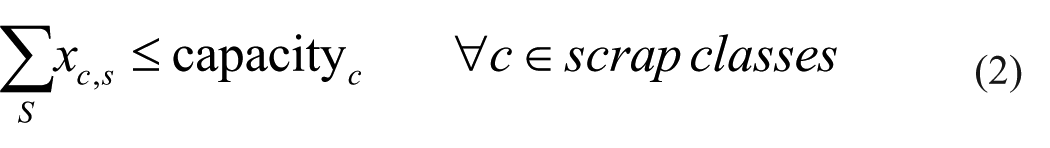
where

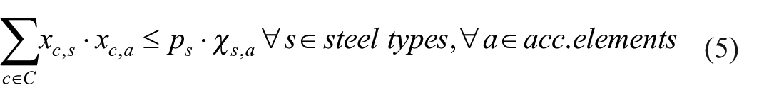
where ks defines how much steel of a specific steel quality

where
Furthermore, to prevent the optimisation algorithm from minimising the energy levels by setting all scrap usage amounts to zero, a constraint demands a minimum fraction
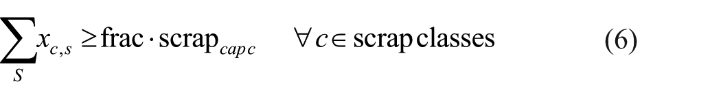
where
where
Results and discussion
Recordings in the hyperspectral laboratory were conducted using the SWIR camera with 437 usable channels together with the three channel RGB camera to analyse desired materials in the metal residue stream as well as foreign and contaminant materials. All investigated steel-related materials exhibited partially rusted surfaces. In the RGB image, which is used just for human inspection, only the rust or the colour of the particles is visible, without any information about the material. In contrast, the SWIR technology significantly enhances the available information by revealing details about the material, also beneath the rust. This capability of SWIR technology enables a deeper and more precise analysis of material composition, which is particularly beneficial in industrial applications.
However, the confusion matrix in Figure 5 indicates an overlap between metal classes in the SWIR measurements. Examples are the copper and aluminium classes, since only 23.4% of copper samples are correctly identified and 38.39% are misidentified as steel, whereas aluminium shows a 69.09% correct rate with 10.36% confused as steel. This data suggest the SWIR measurement alone yields limited discrimination between metal classes. Further spectral or other measurement approaches would be necessary to improve separability. As only the intensity of the spectral information differs, separation can only be achieved by multi-modal analysis including colour information and/or shape analysis.
Samples were taken in 4 series, manually sorted, and assigned to 1 of 14 material classes steel, aluminium, copper, metal with dark rust, metal with light rust, painted metal, drink can, stone, wood, painted wood, plastic, rubber, Styropor, and fabric. The class steel is considered the desired class, whereas all others are foreign or contaminant materials. The statistics of Figure 3 show that the materials are not equally represented, for instance steel is overrepresented. For each of the 4 recording series, approximately 55 individual scrap samples are available, which have been recorded multiple times in different positions and orientations on the conveyor belt. The scrap samples were placed manually on the conveyor belt, often in different orientations, to create a diverse dataset with respect to reflections, paint or colour, and geometry of the particles. Although the resulting images are processed in patches, it is ensured that all patches of one scrap particle are either part of the training or the test set, but objects are not split between training and test set.

Distribution of pixel percentages across material classes in our full hyperspectral dataset, including both training and testing subsets. The histogram represents the proportion of pixels assigned to each class, highlighting variations in class representation.
The hyperspectral images were pixel-wise class annotated. Figure 3 shows the distribution of pixels across the material classes. Before training, individual objects from the annotated images were extracted, and the objects split into training and test sets at an 80/20 ratio. During training, pixels were randomly sampled for the MLP model and 7 × 7 image patches for CNN-based models, respectively.
Table 2 shows the quantitative results for our three trained models on the test dataset, reporting the average accuracy across all pixels along with macro-averaged precision and recall. The MLP performs noticeably worse compared to both CNN-based models, indicating that incorporating spatial information significantly boosts performance. Furthermore, the 3D-CNN yields higher scores than the 2D-CNN, demonstrating that extending convolutional operations across the spectral dimensions provides an additional performance gain. However, a notable downside of the 3D-CNN is its inference speed, which is approximately five times slower than the 2D-CNN. Despite this drawback, the 3D-CNN was investigated further since it is the best-performing model.
Quantitative results for the three trained models on the test dataset. The table shows the average accuracy across all pixels along with macro-averaged precision and recall.

MLP: multilayer perceptron; CNN: convolutional neural network.
Figure 4 qualitatively shows the classification results of the 3D-CNN model for selected objects from the test dataset. In particular, the results for objects of the steel class shown in the first row are very good. Notably, for the shown aluminium object, most errors occur in regions where the RGB image suggests that the material is highly reflective. Such reflections are challenging to handle, since, in hyperspectral data, the signal can quickly become saturated in these areas, making classification challenging. Furthermore, the classification for the stone object and the circular plastic piece exhibits some pixel misclassifications. However, despite these localised errors, most of the pixels are still correctly classified. Therefore, the material of the entire object can still be accurately identified by applying a simple majority vote across the predictions.
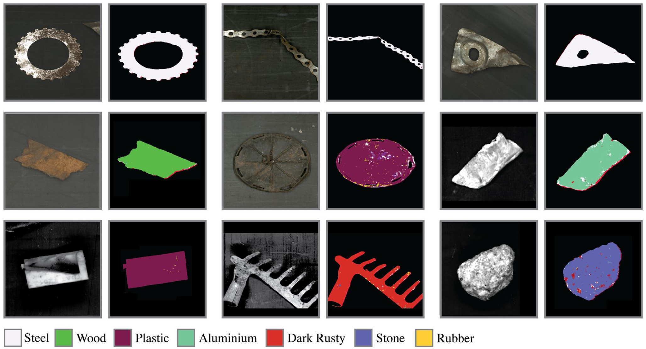
Classification results for a selection of test objects. For each object, the left RGB image was acquired with a four-channel NIR camera for visualisation, whereas the right image displays the corresponding classification output computed from the recorded hyperspectral imaging data.
Figure 5 shows the column-normalised confusion matrix for the 3D-CNN model, where the diagonal entries illustrate the accuracy for each material. Notably, the model performs particularly well in classifying steel, wood, painted wood, dark rusted metal, painted metal, plastic, and fabric. The classification accuracy for copper is relatively low, likely due to the small number of copper samples available during training. Additionally, misclassifications occur among plastic, rubber, and styropor, suggesting a degree of similarity or insufficient differentiation in the learned features for these materials.
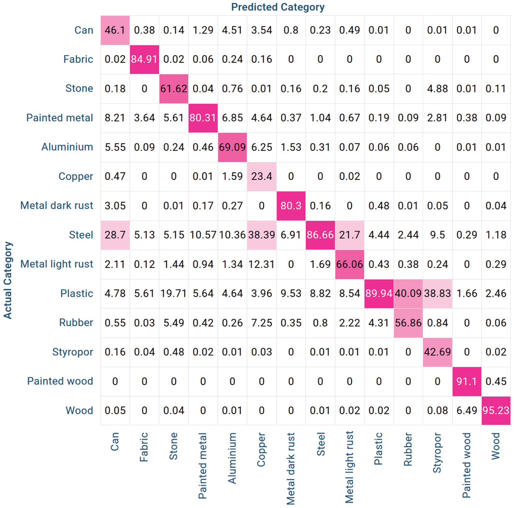
Confusion matrix for the predictions of the 3D-CNN on the test dataset.
The material predictions of the 3D-CNN model are used in the optimisation to quantify the distribution of the scrap classes. Although the model does not directly predict the scrap classes, the share of non-ferrous materials are a reasonable indicator for the scrap classes. This is combined with the parameters, objectives, and constraints to find the most efficient utilisation of scrap metals in storage to produce the required steel classes. It is necessary to specify the available capacity per scrap class, as well as the respective energy needed to melt these classes down to the model as initial condition. The optimisation is able to calculate how many charges of each specific output product can be produced and is expandable indefinitely as long as the necessary information on steel quality and accompanying element limits are defined.
Conclusion and outlook
This work provides insights into the design and test of a scrap classification and optimisation pipeline in steel scrap recycling. The objective is to detect the steel composition, so that the steel making process can be adapted to changing scrap compositions and contaminants. The pipeline starts with hyperspectral image capturing, includes deep learning methods for image recognition, and uses the detected scrap composition in a final optimisation step.
The hyperspectral imaging shows that the separation between metals and foreign or contaminant materials in the SWIR range works very well, for instance, detection of stone or wood particles. However, a highly reliable separation of the individual metal types needs support by visible range detection, since the reflectivity of metals differs in the visible spectrum and levels for longer wavelengths as shown in Tong et al. (2016; Figure 1). The image capturing system with its multiple cameras, lighting, and conveyor belt proved valuable in recoding the images in a quantity and quality necessary for the sub-sequent image recognition. The image recognition itself evaluated three distinct deep learning models differing in their architecture and therefore also complexity. Both qualitative and quantitative evaluations show promising results for classifying material classes in scrap using the spectral information for the images. In particular, the good performance for steel classification is promising and especially significant. Given that steel is the primary material class of interest for our use case. A clear recommendation for the use of the 3D-CNN over the MLP and 2D-CNN can be given. However, the greater inference complexity can be a limiting factor in industrial application, since this either causes higher costs for the computing hardware or greater latencies. The optimisation of scrap compositions selected the best possible scrap usage given the boundary conditions of a specific steel plant. Therefore, it supports cost reduction and further automation in the plant operation and is also a valuable tool to qualify the costs of increasingly using post-consumer scrap fractions of lower purity standards.
This publication is a good basis for future work in all three investigated parts. Starting with the hyperspectral imaging, a promising next step is the determination of key wavelength to design the most efficient recording system. The development of recording equipment robust enough to be installed in the harsh condition of a steel plant is also essential for industrial applications. Then, images can be recorded directly in the recycling process since the image capturing system is improved to cope vibrations, stray light, contamination, etc. of such an industrial environment. The collected dataset is expected to be much larger with an increased diversity of objects for training and testing. A larger dataset would enable using more sophisticated deep-learning methods. For instance, transformer-based models have demonstrated strong performance in hyper spectral classification but require relatively large amounts of training data. Finally, also the optimisation has to be extended to handle the industrial conditions. Although the numbers in this work specifying energy demand, additive consumption, furnace capacity, etc. have been selected close to real steel plants in Austria, many aspects of industrial steel recycling have been simplified, like scheduling order of different charges, variable energy costs, or shift planning of the workers.
Footnotes
Acknowledgements
The authors like to thank Stefan Körner for the discussions and ideas.
Author contributions
Heimo Gursch: Writing – Review & editing, Methodology, Writing – Original draft, Conceptualisation.
Andreas Ofner: Writing –Original draft, Software, Investigation.
Robert Harb: Writing – Original draft, Software, Investigation, Conceptualisation, Methodology.
Malte Jaschik: Writing – Original draft, Investigation, Conceptualisation, Project administration.
Harald Ganster: Funding acquisition, Conceptualisation, Supervision, Methodology.
Johannes Rieger: Writing – Original draft, Validation.
Funding
The authors disclosed receipt of the following financial support for the research, authorship, and/or publication of this article: This work is funded by the project ‘InSpecScrap – INtelligent multi-SPECtral characterisation for material analysis on SCRAP yards’ (No. 1510) funded by the Future Fund of the State of Styria (‘Zukunftsfonds Steiermark’). Additional funds are from the project ‘REDUCE – REDUCEed carbon footprint using explainable AI for human empowerment in design/engineering and production’ (No. FO999925795) funded by the Austrian Research Promotion Agency (FFG). Know Center is a Competence Center for Excellent Technologies (COMET) competence centre that is financed by the Austrian Federal Ministry of Innovation, Mobility and Infrastructure (BMIMI), the Austrian Federal Ministry of Economy, Energy and Tourism (BMWET), the Province of Styria, the Steirische Wirtschaftsförderungsgesellschaft m.b.H. (SFG), the Vienna business agency, and the Standortagentur Tirol. The COMET programme is managed by the Austrian Research Promotion Agency FFG. K1-MET competence centre gratefully acknowledges the funding support by COMET, the Austrian programme for competence centres. COMET is funded by the Federal Ministries BMIMI and BMWET, the Federal States of Upper Austria, Tyrol and Styria as well as the Styrian Business Promotion Agency (SFG) and the Standortagentur Tirol. Furthermore, Upper Austrian Research GmbH continuously supports K1-MET.
Declaration of conflicting interests
The authors declared no potential conflicts of interest with respect to the research, authorship, and/or publication of this article.