Is It Good to Be Green? Assessing the Ecological Results of County Green Infrastructure Planning

Abstract

This study assesses the process and outcomes of landscape-scale green infrastructure planning as a strategy for supporting biodiversity and ecosystem services. The research examines how nine county planning agencies carry out green infrastructure planning and the effectiveness of those strategies in retaining, preserving, and connecting green space over time. The study develops and applies a new framework for green infrastructure planning and uses remote sensing, land conversion analysis, and a landscape ecology–oriented spatial analysis program (FRAGSTATS) to assess on-the-ground change. Results confirm the relationship between green infrastructure planning and green space outcomes, question conventional metrics, and highlight the importance of strategies that support connectivity and manage growth.

Keywords

green infrastructure green space ecosystem services connectivity conservation networks

Recent projections by the U.S. Census Bureau suggest that the U.S. population will increase by nearly 90 million people by 2050 (United States Census Bureau 2012). Given predominant settlement patterns, many communities will accommodate this growth through greenfield development. This strategy converts and degrades lands that provide critical ecosystem services such as habitat, climate regulation, and air and water purification. The forests, wetlands, and other landscapes that provide these services comprise a community’s green infrastructure, a fundamental part of healthy, livable, and resilient communities (Randolph 2004; Benedict and McMahon 2006). In recent years, the term green infrastructure has been used principally to describe the “greening” of urban infrastructure, often with the objective of managing stormwater. This study uses the term more broadly to reference land that supports natural systems, regardless of form, scale, ownership, or level of protection. The interpretation acknowledges the importance of large-scale green space and conservation networks, those that most effectively provide many of the services on which we and other organisms depend.

According to the United States Forest Service, “conversion of forest land to commercial and residential use is increasingly affecting the ability of ecosystems to provide basic services” (Small and Lewis 2009, 1). Much of this impact is due to poor local planning, weak land use controls, and short-sighted decisions that favor development. Research shows that factors such as landscape fragmentation that degrade ecosystems—and consequently their ability to provide services—“occur at the local level and are generated by local land use decisions” (Brody 2003, 512). But the connection between local land use planning and green infrastructure works both ways. If local government planning, land use regulations, and decision-making can cause the problem, they can also be the solution.

In response to the growing understanding of the many benefits of green spaces, local governments are increasingly adopting programs and policies designed to protect or enhance lands that provide ecosystem services. Collectively, these strategies can be classified as green infrastructure planning. But despite the fact that green infrastructure planning is on the rise—and increasingly important given the uncertainty surrounding climate change—there have been few overall assessments of the effectiveness of current approaches to supporting green space networks.

This study addresses this gap by examining green infrastructure planning strategies and their ecological results over time. It details the plans, implementation techniques, and outcomes of nine counties with different levels of green infrastructure planning to determine the on-the-ground impact of green infrastructure strategies. The study then provides recommendations for local governments that are seeking to improve their green space planning and create healthy, resilient, and biologically diverse regions. The two organizing questions are (1) Are county planning agencies that employ many green infrastructure planning strategies more effective at retaining green space, preserving ecologically significant lands, and supporting connectivity than those that employ fewer strategies? and (2) If they are, what makes the difference? Budget shortfalls, ecological uncertainties, and population growth suggest that the efficient use of conservation dollars and effective support of ecosystem services are as important as ever. So, as public funding is likely to remain constrained, while the number of communities adopting green infrastructure planning increases, it will be critical for local governments to focus on strategies that most clearly maximize ecological services over time.

Two Aspects and Three Challenges of Assessing Green Infrastructure Planning

Two aspects of large-scale green infrastructure planning distinguish it from other environmental planning efforts. The first is a broad focus on natural systems, ecological function, and associated ecosystem services (McDonald et al. 2005). The second is planning and land development strategies that emphasize green space characteristics that support those services (Randolph 2004). Of the two characteristics, the first—the simplest to understand and implement—dominates the field both in theory and practice. The second is less well documented and is the focus of this study. While research on how counties can protect and retain important green spaces is common, most studies emphasize mapping and analysis, often with the objective of prioritizing land for preservation (Walmsley 2005; Weber, Sloan, and Wolf 2006). Such studies usually mention implementation as a next step, but do not assess on-the-ground outcomes. So while the body of literature surrounding green infrastructure planning has grown significantly in the past ten years, the majority of published research is theoretical. Empirical research on the variety of strategies that comprise green infrastructure planning, and their long-term success in creating green space networks with desirable characteristics, is minimal.

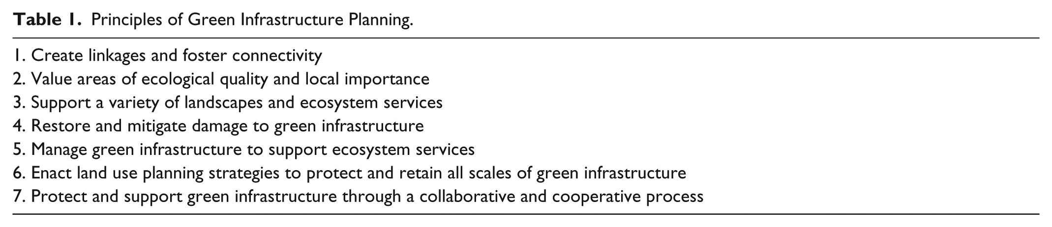
A rigorous analysis of the success of green infrastructure planning over time faces three challenges. The first is how to define success in a clear and practical way. The Conservation Fund (TCF), a leader in green infrastructure planning, suggests three attributes for assessing green infrastructure planning: (1) landscape-scale; (2) driven by public process; and (3) resulting in a strategy intended to protect an ecological network (McDonald et al. 2005). Other researchers have suggested strategies that are holistic, multifunctional, interconnected, contextual, and value quality over quantity (Sandstrom 2002; Benedict and McMahon 2006; Erickson 2006; Kambites and Owen 2006; Tzoulas et al. 2007). From a local land use planning perspective, these can be translated into seven action-oriented principles of green infrastructure planning (see Table 1).

Table 1.

Principles of Green Infrastructure Planning.

1. Create linkages and foster connectivity

2. Value areas of ecological quality and local importance

3. Support a variety of landscapes and ecosystem services

4. Restore and mitigate damage to green infrastructure

5. Manage green infrastructure to support ecosystem services

6. Enact land use planning strategies to protect and retain all scales of green infrastructure

7. Protect and support green infrastructure through a collaborative and cooperative process

The specificity of the principles is important as it helps to overcome the second challenge of assessing green infrastructure planning: time frame. A temporal mismatch exists between planning actions and their effects. The vast majority of local governments have instituted green infrastructure plans and programs only in the last five to seven years, meaning efforts are too recent to have been implemented completely, much less yield measurable on-the-ground impacts. This study overcomes that limitation by examining local government programs that may not be explicitly labeled “green infrastructure planning” but have incorporated the key principles that define it. Local governments have been planning in support of green space for over a century. The inclusion of strategies under other headings acknowledges that legacy. Including green infrastructure strategies that may not be labeled as such also enables the study to examine mature green infrastructure efforts—activities that began around 2000—and related change in on-the-ground green space. Although ten years is a short period of time, ecologically speaking, longer-term studies would include more changes in planning strategies and implementation techniques and further confound results. The length of this study balances the time scales of environmental outputs and local government actions.

The third challenge is measuring outcomes. Ecological systems are complex and ecosystem services are notoriously difficult to measure. There are many variables at play and it is difficult to conclusively link environmental outcomes with planning actions. Here, ecology and conservation biology provide a critical link. Decades of research in these fields confirm that the environmental outcomes of a conservation network are largely a result of the characteristics of that network, the extent and qualities of which can be measured far more easily. Consequently, while the outcomes of green infrastructure planning may be difficult to measure, the outputs in the form of the resultant green spaces are comparatively easy to identify. This study leverages that connection by using green space network characteristics as indicators rather than attempting to directly measure ecosystem services and environmental quality outcomes. These metrics simplify complex and dynamic natural systems to a series of discrete, point-in-time measurements. They capture only a portion of the impact of green space planning activities, and do not fully account for local and seasonal variation; but they provide a good foundation for understanding green infrastructure outcomes over time. In short, if the benefits of a community green infrastructure program are derived from specific landscape characteristics, the most straightforward way to understand the program’s effectiveness is to measure the gain/loss of those characteristics over time (e.g., land conversion, landscape connectivity). It is also an appropriate strategy for local communities that are interested in understanding green space success but lack the in-depth natural systems data that would be necessary to measure ecosystem services directly.

Important Green Space Characteristics in the Literature

The objective of landscape-scale green infrastructure planning is to ensure adequate ecosystem services by delineating, preserving, and maintaining a functional green space network (Benedict and McMahon 2006; Kambites and Owen 2006). Since the benefits of a green infrastructure network are naturally derived, their provision depends upon the network’s ecological characteristics. And because green infrastructure covers only a portion of the landscape, communities must think carefully about the attributes of the network they are creating and implications for ecosystem services. In doing so, communities have decades of ecological research at their disposal. The connections that research (summarized below) makes between key green space characteristics and environmental quality and services enables the assessment detailed in this study.

Research in the fields of landscape ecology and conservation biology indicates that there are three main characteristics that impact the ecological success of a conservation network: quality, size/shape, and connectivity. Large, undisturbed natural areas provide services more effectively and efficiently than smaller degraded areas, mainly because they contain a greater amount of core area—interior area that is not impacted by surrounding land uses—and cover a larger percentage of the natural landscape (Forman 1995). Landscape ecology research shows that large patches of a land cover type—for example forest—have more interior species (which are usually the most sensitive), larger interior species populations, lower probabilities of species extinctions, greater overall diversity of habitats and species, greater coverage of species ranges, more natural disturbance regimes, and more comprehensive cover of important natural features than small patches (Harris 1984; Shafer 1990; Opdam 1991; Forman 1995). The shape and proximity of natural areas is also important. Irregular or geometric (e.g., square) features have a higher proportion of edge area than rounder shapes. The increased edge area means increased interaction with surrounding land uses and increased diversity of edge species—which tend to be in abundance in the landscape overall. In addition, green spaces that are close together provide for more movement of species between patches and more continuous protection of features (ibid.). In their landscape ecology synthesis for land use planning, Dramstad, Olson, and Forman (1996) identify the “ecologically optimum patch shape” to be an amoeboid structure with a large rounded core, a few irregular bumps and dips along the boundary to enhance edge species diversity, and connective corridors leading to adjoining patches.

In landscapes that are fragmented by development, corridors between green spaces allow for movement of species and environmental flows (Dramstad, Olson, and Forman 1996). There has been considerable debate over the years on whether corridors provide support for species diversity and populations (Simberloff 1992; Beier and Noss 1998), but enough studies support their ecological benefits that the concept remains relevant (Tewksbury et al. 2002; Damschen et al. 2006). Green infrastructure networks are usually conceived as a system of hubs and links, a configuration adapted from landscape ecology and applied by two of the states discussed in this study: Maryland in their 2001 green infrastructure assessment and Florida in 2000 and 2008 (Weber, Sloan, and Wolf 2006; Florida Natural Areas Inventory 2009).

Urban planning and environmental management literature is most robust on actions that support green space quantity results. Furthermore, land preservation practitioners routinely use green space quantity as a success measurement (somewhat pejoratively referred to as “bucks and acres calculus”) (Sawhill and Williamson 2001). Such metrics make no mention of the quality, location, or configuration of protected land. Few studies address the overall quality and connectivity outcomes of green infrastructure planning efforts, but several do examine the outcomes of individual strategies—most commonly land preservation and clustered development.

A variety of land preservation studies describe how conservation organizations can prioritize easements to lands that maximize ecological value per dollar spent (Ando et al. 1998; Abbitt, Scott, and Wilcove 2000; Newburn, Berck, and Merenlender 2006), but most are applied statistical studies and mainly theoretical. One notable empirical study out of Larimer County, Colorado, suggests that city and county open space programs are more effective at fostering connectivity than biodiversity or agricultural values, but are more successful at preserving biodiversity than nongovernmental organizations (Wallace et al. 2007). Wallace and colleagues also found that land preservation was more effective at supporting high or outstanding biodiversity than clustered development. Other studies suggest that clustered development provides minimal quality and connectivity benefits over conventional subdivision development (Nassauer et al. 2004; Lenth, Knight, and and Gilgert 2006; Milder, Lassoie, and and Bedford 2008). Many local planning tools rarely appear in the literature in the context of green infrastructure outcomes, even though they have implications for ecological quality and connectivity at the landscape scale.

Research Design and Methods

This study assesses the differences in outcomes between local planning agencies that are highly involved in green infrastructure planning and those that are not and identifies the local planning strategies and implementation techniques that make the difference. It does so through a comparative approach—a quasi-experimental multiple case study analysis. The study includes a pretest (2000) and posttest (2010), and a qualitative examination of three sets of three case studies, grouped by state and other attributes. The study highlights the outcomes of high- versus low-level green infrastructure planning in the three states. A framework to measure green infrastructure planning success provides additional clarity and allows for identification of strategies that could improve green space outcomes.

This paper limits the discussion to changes in county forestland and other natural land types. Counties, rather than cities, are the appropriate unit of analysis because landscape-scale green infrastructure planning emphasizes natural areas, open spaces, and large-scale green space networks, and counties simply have much more land of this type under their jurisdiction. For a similar reason, most large-scale green infrastructure planning takes place at the county level. The overarching hypothesis (hypothesis 1) is that county planning agencies that employ many of the strategies and implementation techniques associated with green infrastructure planning will be more effective at retaining, protecting, and connecting green infrastructure over time than county planning agencies that employ fewer strategies and techniques. A strong relationship between the level of green infrastructure planning and green space success disproves the null hypothesis that there is no difference in on-the-ground green space outcomes between county planning agencies that apply many green infrastructure planning policies and strategies and those that employ few in favor of the alternative.

The study includes two main components: (1) creating and applying a green infrastructure planning framework and (2) assessing the on-the-ground outcomes of green infrastructure planning in nine case counties: Baltimore, Anne Arundel, and Charles Counties in Maryland; Leon, Alachua, and Marion Counties in Florida; and Boulder, Arapahoe, and Adams Counties in Colorado. The inclusion of three states and three counties (in each state) balances practical and methodological considerations. Fewer than three states or counties resulted in insufficient replication and more than three presented increasing categorization, comparability, and data acquisition challenges. The included states were chosen for their progressive and mature green space planning and the availability of natural resources data. Counties were selected for their matching size and growth characteristics and varying levels of green infrastructure planning. All nine counties had populations greater than one hundred thousand in 2000, which grew by at least 5 percent over the study period, and fall within the same general region of their state. For example, the Colorado counties are within the Front Range, Floridian counties are inland and in the northern half of the state, and Maryland counties are within the Chesapeake Bay watershed and coastal zone. These similarities ensure that counties within the same state have comparable regulatory environments.

A Framework for Understanding Green Infrastructure Planning

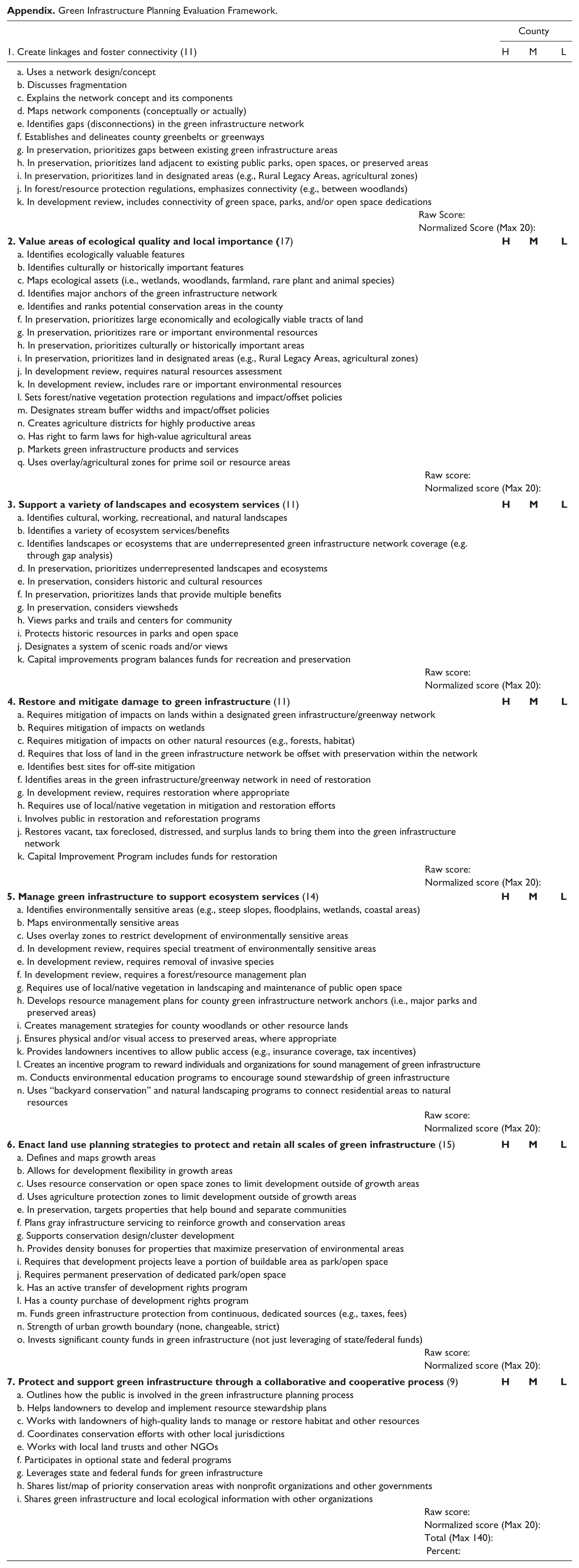
This study uses what could be called a “principle-policy” framework to understand county green infrastructure planning programs. Derived from content analysis and plan evaluation literature (Berke and French 1994; Baer 1998; Berke and Manta Conroy 2000; Brody 2003; Norton 2007), a principle-policy framework is an assessment structure composed of the principles that define an overarching planning goal and implementation strategies that—if integrated into planning practice—would show support for the principles. The more strategies and techniques that a local plan includes, the greater its support for the overarching planning goal. The framework for green infrastructure planning developed through this study—called the Green Infrastructure Planning Evaluation Framework (the Framework)—enables a standardized analysis of the level and relative emphasis of green infrastructure planning in each of the case study counties. Similar frameworks exist for other planning regimes and goals (e.g., smart growth [Edwards and Haines 2007], sustainable development [Berke and Manta Conroy 2000]), but this is the first such framework for green infrastructure planning. The backbone of the Framework is the seven principles of green infrastructure planning described in the previous section. The “policy” portion was populated with strategies, and techniques that support the principles through a review of ten green infrastructure plans written since 2000. The plans are representative of green infrastructure planning throughout the country and include at least one plan from each case state.¹ The review resulted in between nine and seventeen strategies/policies for each of the seven principles, for a total of eighty-eight policies and strategies (see appendix).

The resulting Framework provides a platform for comparison of the case counties and a way to understand how the counties perform relative to national leaders in green infrastructure planning and the principles that define the strategy. To apply the Framework, I reviewed the plans, programs, zoning ordinances, capital improvement programs (only 2004–2010, as they were available for all communities), and subdivision and land development regulations for each of the nine case counties. The review identified the extent to which each county implemented the eighty-eight green infrastructure planning components identified in the Framework. Given that counties may gather information and implement strategies and policies completely, partially, or not at all, results were coded 0, if absent; 1, if present but not required/complete; or 2, if present and required/complete. The scale is a common standard and is used in the majority of plan assessment studies, including those employing principle-policy frameworks (Berke and French 1994; Brody 2003; Edwards and Haines 2007; Evans-Cowley 2009, 2011). Follow-up interviews with local planners in the counties were used when necessary to verify and complete the Framework. While one of the considerations in case selection was the level of green infrastructure planning, the framework also served to confirm designations of “high,” “moderate,” and “low” green infrastructure planning effort.

The primary objective of green infrastructure planning is to protect and maintain green spaces that provide critical ecosystem services. The clearest indicator of county green infrastructure planning success, then, is a locality’s ability to retain or enhance green space characteristics that are supportive of such services, specifically (1) retain green infrastructure, (2) retain or protect high-quality green spaces, and (3) maintain or increase network connectivity.

Assessing On-the-Ground Change: Quantity

This study examines changes in the quantity of green infrastructure between 2000 and 2010 using remote sensing and GIS analysis of Global Land Survey (GLS) data. It uses three different vegetation indices (Normalized Difference Vegetation Index [NDVI], Normalized Built-Up Index [NDBI; Waqar et al. 2012], and a third unnamed combination of bands 5 and 7 [Ozesmi and Bauer 2002]) to classify orthorectified leaf-on 30m Landsat TM and ETM+ satellite images for each of the nine counties into simple land use/land cover maps. Resulting maps include four categories: forest/grassland/wetland (depending upon the county), agriculture, development, and water. Accuracy of the maps was verified by hand and adjusted, when necessary, to reflect on-the-ground conditions. Differencing the 2000 and 2010 maps showed change in landscape type and configuration, including the most significant change—the conversion of land from natural to developed uses. Change estimates can be considered conservative as a two-cell (60m) negative buffer was used on change areas. Negative buffers reduce the size of an output area by a specified distance. Their use here accounts for land use differences that were due to year-to-year variations in temperature, rainfall, and annual image dates rather than development or re-growth.

Assessing On-the-Ground Change: Quality

The quality of green infrastructure also impacts its ability to support ecosystem services. One way for a county to protect high-quality land is to use zoning and subdivision and land development regulations to guide development away from critical ecosystem service areas and toward more marginal lands. Another way is to permanently preserve high-quality areas through fee simple purchase or the acquisition of conservation easements from willing landowners. This study examines both by comparing the ecological quality of lands developed between 2000 and 2010 to that of locally protected lands (as opposed to state or federal lands) in the same county. The metric “difference in quality between protected and developed land” or DiQ is unique to this study. While areas of a state may be similar, and many of the counties used in this analysis are located in the same region, no two counties have the same environment. Natural systems are complex and naturally variable. The DiQ metric accounts for some of that variability by comparing ecological qualities within each county, rather than between counties.

State planning and natural resources departments in Maryland, Colorado, and Florida make available a variety of geographically referenced natural resource information that can be combined into an “ecological value” GIS layer. In Maryland, such an index already exists. The Department Natural Resource created a GIS layer called “green infrastructure ecovalue,” as part of the state’s 2001 Green Infrastructure Assessment (Weber 2003). It is composed of high-value and sensitive areas such as interior forest, wetlands, and stream valleys, in addition to key green infrastructure hubs and links, combined and scaled from 0 to 100. The data are available through the agency’s website and provide information on the relative ecological importance of each 30m by 30m cell in the Maryland grid. Calculating DiQ required creating similar layers for Florida and Colorado. Creating identical ecovalue layers for Florida and Colorado would be impossible, but also undesirable. Each state has different physiographic regions, ecosystems, species, programs, and interests. Consequently, each collects information on—and values—environmental systems differently. In creating ecovalue layers for Florida and Colorado, this study followed Maryland’s methods but used different data layers when analogs to those provided by Maryland were unavailable or inappropriate or the state valued different species or natural characteristics. The three ecological value layers included the same methods, most of the same components, and the same 0 to 100 scale.² Furthermore, since comparisons are between counties in the same state, rather than between states, small differences between state ecological value layers are not significant.

Assessing On-the-Ground Change: Connectivity

A robust green infrastructure network is interconnected, particularly within individual land use types, such as farmland or forestland. This study examines connectivity from the perspective of landscape ecology, which envisions landscapes as series of patches, hubs, and linkages and uses a variety of metrics to measure the spatial arrangement of landscape elements, particularly patches—contiguous areas—of forestland and farmland. There is a robust literature surrounding the selection of composition and configuration metrics, but the overwhelming consensus is that metrics must be carefully selected to align with the landscape processes being studied (Li and Wu 2004). A variety of landscape metrics provide appropriate composition and connectivity information and are supported broadly by landscape assessment literature (Riiters et al. 1995; Hargis, Bissonette, and David 1998; Li and Wu 2004; Leitao et al. 2006). The list of selected metrics (see Table 2) emphasizes measures that are known to be useful for planning applications (Leitao et al. 2006) and those available in FRAGSTATS, the raster-based spatial analysis program used to carry out the analysis. The emphasis of this study is the connectivity of individual land use classes, so all metrics of interest are at the class level, which averages values for all patches of a certain land use/land cover type.

Table 2.

Metrics Used to Assess Landscape Connectivity.

Metric	Type	Purpose
Mean radius of gyration	Area-edge metric	Measures the mean patch extensiveness (how far a patch extends) for each class (larger patches have a larger radius of gyration); the average distance a landscape can be traversed without leaving the patch
Mean shape	Shape metric	Measures the mean geometric complexity (irregularity) of patches in each class
Mean Euclidian nearest neighbor	Aggregation metric	The average distance between a patch of a certain class and its nearest neighbor of the same class
Proximity	Aggregation metric	Measures patch isolation based upon the size and distance of like patches; provides information on the distribution of patches of each type across the landscape; defined search radius of 1,000 meters

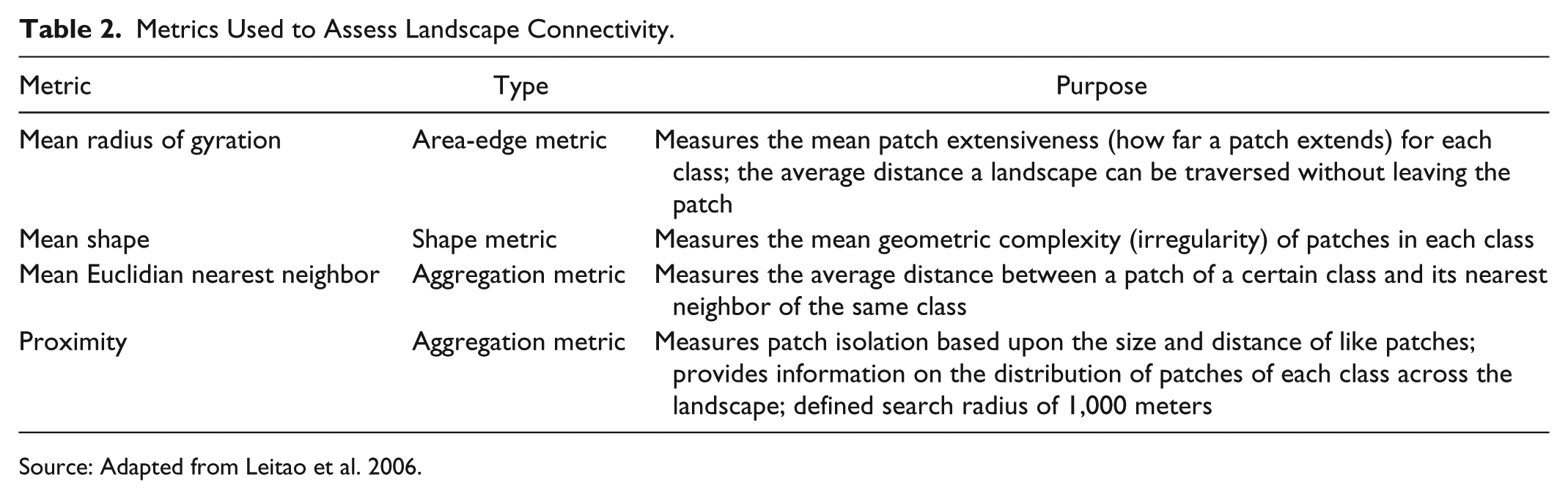
Source: Adapted from Leitao et al. 2006.

Does Green Infrastructure Planning Lead to Better Outcomes?

Results suggest that it is “good to be green” in Colorado, Florida, and Maryland. The relationship between level of green infrastructure planning and green space outcomes in the nine case study counties is strong enough to reject the null hypothesis and support the alternative hypothesis that counties that employ many green infrastructure policies and strategies are more effective at retaining green space quantity, quality, and connectivity over time than those that use fewer. In general, counties with a high level of green infrastructure planning exhibit a high level of success in the three outcome categories and low-level counties show the least success, with moderate counties falling in the middle. When the high-level county in a state performs best, the moderate-level county performs moderately, and the low-level county falls behind, the ordering for that state can be described as following the expected H/M/L ordering. Colorado has the strongest trend; it follows the H/M/L ordering of results, which indicates a strong relationship between green infrastructure planning level and outcomes. Maryland exhibits the second strongest relationship between level of green infrastructure planning and green space outcomes, with one divergence from the H/M/L ordering, and Florida is third with two divergences. Assessments of high, moderate, and least success in green infrastructure outcomes are relative and apply only within each state. But examining the overall trends in each state provides information on green infrastructure planning outcomes and what may cause deviations from the H/M/L ordering in some states and not in others.

Quantity

The level of a county’s green infrastructure planning clearly relates to its ability to retain green infrastructure over time in Colorado and Florida and to a lesser extent in Maryland as well. Only Baltimore County (H) and Anne Arundel County (M), Maryland, did not follow the H/M/L ordering. Results suggest that green space planning has the greatest impact in moderate and slow-growing counties, particularly where green infrastructure programs are mature and robust (see Table 3). This is particularly true of Boulder County, Colorado (H), and Baltimore County, Maryland (H), which grew in population by 8.4 and 6.7 percent over the study decade (compared to 9.7 percent nationwide) and increased in developed area by a modest 2 and 8 percent, respectively. Both counties are known for their strong land preservation programs and mature growth management regimes. For example, while Baltimore County (H) lost slightly more natural land to development than Anne Arundel (M) over the study period, unlike Anne Arundel, newly developed lands were mostly within the county’s urban services boundary. For counties with growth rates double that of comparable localities (i.e., Charles County, Maryland, and Marion County, Florida) and low levels of green infrastructure planning, planning appears to have had a minimal impact on developed area per capita.

Table 3.

Growth and Development Statistics for Counties in Colorado, Florida, and Maryland between 2000 and 2010.

	Colorado			Florida			Maryland
	H	M	L	H	M	L	H^a	M^a	L
Population added	23,000	84,000	77,700	36,000	29,400	74,400	51,000	48,000	25,000
Growth rate (%)	8.40	17.20	21.40	15	13.50	28	6.70	9.80	21.60
Increase in developed area (%)	2	28	26	22	22	34	8	7	25
Land developed (per capita added)	.04 ac	.08 ac	.12 ac	.12 ac	.25 ac	.58 ac	.18 ac	.15 ac	.50 ac

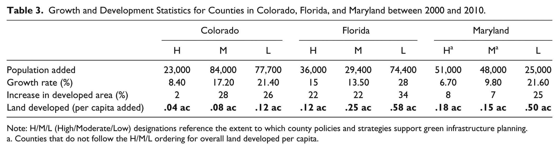
Note: H/M/L (High/Moderate/Low) designations reference the extent to which county policies and strategies support green infrastructure planning.

Counties that do not follow the H/M/L ordering for overall land developed per capita.

Quality

The level of green infrastructure planning a county employs also relates to green space quality, as indicated by DiQ metrics. For natural lands—forest, wetland, and grassland—all three states generally follow the H/M/L ordering (see Figure 1). In Florida, while the ordering holds, there is little variation between high- and moderate-level counties. Leon (H) and Alachua (M) have the same—relatively high—level of success. But they do both outperform Marion County (L). The overall result is that green infrastructure planning helps to protect high-quality green space over time, but the total acreage and quality of green space—protected or not—also has an impact.

Figure 1.

Difference between the area-weighted mean ecovalue of natural lands that were developed between 2000 and 2010 and those that were protected.

There are two major results from this analysis. First, in all cases, there was some difference in the ecological quality between developed lands and protected areas. All nine counties succeeded in protecting higher quality lands than they developed, to some extent. The smallest difference was 3, for Adams County, Colorado, but the low value is similar to that of Arapahoe County. Natural areas in both counties are largely grassland, which is less variable in quality than other types of natural land. Second, the extent of high-quality natural area in a county—particularly forestland—impacts overall ecological value, which inflates differences between protected and developed lands. Two counties that performed better than expected are Marion County, Florida, and Boulder County, Colorado. While Marion (L) was the lowest-performing county in Florida, it was generally successful at retaining high-quality lands. And while most high- and moderate-level counties performed similarly, the developed/preserved land difference for Boulder (H) was double that of the moderate-level green infrastructure planning county in Colorado. The most likely explanation is that the two have very large forested areas. Marion County has Ocala National Forest, the second largest national forest in the country, and the western half of Boulder County is mountainous and heavily forested, with large sections that are publicly owned. Large hubs of forest have significant core area and are highly supportive of biodiversity, particularly when not fragmented by other types of development, which is true of forests in Boulder and Marion.

Connectivity

Patch metrics for the nine counties indicate that there is also a relationship between the level of green infrastructure planning a county employs and the county’s success in retaining or improving connections between green spaces. Results also further confirm the importance of large hubs and a critical mass of green space in anchoring a green infrastructure network.

The only two counties that deviated from the H/M/L ordering were Alachua County (M) and Marion County (L), Florida (see Table 4). The explanation again is Ocala National Forest. The Forest covers the eastern half of Marion and is one large contiguous hub. That portion of Marion is perfectly connected. Because metrics are area-weighted, the Ocala National Forest provides Marion County enough base connectivity that significant fragmentation in the western half of the county—which has less forest to begin with—has less impact than forest fragmentation does in Alachua. The Cross-Florida Greenway also bisects Marion, providing additional connectivity. Alachua County had less fragmenting development than Marion, but with far less state and federal green space experienced more loss of connectivity. The result shows the importance of preserving large hubs of green space. The areas serve as anchors for a green infrastructure network and bolster overall connectivity.

Table 4.

Interpretation of Change in Landscape Metrics between 2000 and 2010 for Natural Lands in Nine Counties in Colorado, Florida, and Maryland.

	Colorado			Florida			Maryland
Metrics	H	M	L	H	M	L	H	M	L
Patch length (GYRATE_AM)
Patch shape complexity (SHAPE_AM)
Index of patch size and distance (PROX_AM)

Note: Includes only metrics that showed change from 2000 to 2010. White = minimal change; More Shading = greater change.

What Contributes to the Positive Relationship?

Results indicate a positive relationship between the level of green infrastructure planning a county employs and its green space outcomes over a ten-year period. The completed Green Infrastructure Planning Evaluation Framework identifies likely causes of this outcome. Framework results by state show which of the seven green infrastructure planning principles exhibit the greatest variation in score between high-level and low-level green infrastructure planning counties. A large score difference suggests that the principle is one of high variation and likely to make a difference in green infrastructure planning outcomes.

Framework result differences for Colorado, Florida, and Maryland range from 1 to 11, with a natural break (low-frequency point) in the middle, at 6 (see Table 5). Principles with a maximum score difference greater than 6 in more than one state are most likely to influence the differences in green infrastructure planning outcomes. Two principles fit this criterion: 6 = Enact land use planning strategies to protect and retain all scales of green infrastructure, and 1 = Create linkages and foster connectivity. Based on score variation and overall outcomes, these two facets of green infrastructure planning have the greatest potential impact on outcomes.

Table 5.

Maximum Framework Score Difference by Principle for Nine Counties in Florida, Maryland, and Colorado.

Green Infrastructure Principle	Florida Framework Score (Out of 20)			Maximum Score Difference
Green Infrastructure Principle	Leon (H)	Alachua (M)	Marion (L)	Maximum Score Difference
Create linkages and foster connectivity^a	14	8	3	11
Value areas of ecological quality and local importance	11	12	7	4
Support a variety of landscapes and ecosystem services^a	14	10	6	8
Restore and mitigate damage to green infrastructure^a	11	10	4	7
Manage green infrastructure to support ecosystem services	14	14	9	5
Enact land use planning strategies to protect and retain all scales of GI^a	13	12	6	7
Protect and support GI through a collaborative and cooperative process	12	12	8	4
	Maryland Framework Score (Out of 20)
	Baltimore (H)	Anne Arundel (M)	Charles (L)
Create linkages and foster connectivity^a	13	14	7	7
Value areas of ecological quality and local importance	15	11	10	5
Support a variety of landscapes and ecosystem services	10	7	5	5
Restore and mitigate damage to green infrastructure	7	6	5	2
Manage green infrastructure to support ecosystem services	12	8	9	3
Enact land use planning strategies to protect and retain all scales of GI^a	15	13	5	10
Protect and support GI through a collaborative and cooperative process	15	12	10	5
	Colorado Framework Score (Out of 20)
	Boulder (H)	Arapahoe (M)	Adams (L)
Create linkages and foster connectivity	7	6	6	1
Value areas of ecological quality and local importance	12	11	12	1
Support a variety of landscapes and ecosystem services	15	9	9	6
Restore and mitigate damage to green infrastructure	7	5	4	3
Manage green infrastructure to support ecosystem services^a	12	9	8	4
Enact land use planning strategies to protect and retain all scales of GI^a	18	14	9	9
Protect and support GI through a collaborative and cooperative process^a	16	12	9	7

Note: GI = green infrastructure.

Principles with score differences greater than 6.

Connectivity Planning: The Piecemeal versus the Landscape Approach

The Framework includes eleven planning strategies and implementation techniques under the connectivity heading (see Appendix). Many are related to the general culture of green infrastructure planning and whether a given county plans green infrastructure using a network concept. The first, “uses a network design/concept,” exhibits the greatest variation among counties and could make the most difference. Counties that do not use a network concept will have difficulty achieving positive connectivity outcomes. Yet, only four of nine counties clearly use the strategy in their planning documents. The same is true of “maps green infrastructure network components (conceptually or actually).” Most counties map some network components, say state and federal land, but overlook private green space, potential open space, or other types of green infrastructure. Only three of nine counties extensively map green infrastructure networks. Related, only three counties establish greenways or green corridors, which are a useful way to guide future land use decisions.

Nearly all counties in the study consider connectivity in prioritizing land for preservation and in delineating open space dedications in the subdivision or site planning process. Most planning documents mention fragmentation, at least in passing, and include a map with existing green infrastructure components such as parks and other protected areas. These strategies are the status quo of planning for connectivity in the nine study counties. But they are piecemeal rather than network approaches. Each of the four strategies considers green space one parcel at a time rather than as a countywide system.

Implementation techniques with a landscape approach are characteristic of higher-level green infrastructure planning counties. The three high-level counties (and one moderate-level) use a network design or concept for their green space planning, and most go a step further to identify critical connections or gaps in protection of that network. Consequently, they outperform the remaining counties in retaining connections. Without a large-scale understanding of green infrastructure interconnections—protected or not—a county cannot adequately target protection to support connectivity. But, while an open space or green infrastructure plan is one way to support such a system, plans are not always effective. In this study, counties without explicit green infrastructure plans outperformed counties with them, likely because of a lack of implementation of plan recommendations. Regulatory strategies were more characteristic of high-performing counties (e.g., Baltimore County [H], MD, and greenway protection).

Growth Management and Land Preservation: Individual versus Synergistic

The Framework includes 15 strategies and implementation techniques that indicate support for Principle 6: Enact land use planning strategies to protect and retain all scales of green infrastructure. The majority relate to growth management. Most of the case study counties use growth management strategies to minimize the spread of development into rural resource areas and define and map growth areas and support them with gray infrastructure planning. Many also fund open space acquisition from a dedicated source such as sales tax revenue, which is indicative of high levels of resident support for green space.

Purchase of development rights (PDR) programs and, more broadly, open space preservation programs are common among the counties. Counties with older land preservation programs (i.e., Boulder County, CO, and Baltimore County, MD) have tens of thousands of acres of preserved land (see Table 6). Preserved acres are not the only important aspect of green infrastructure planning, but an active land preservation program is a good indicator of broader dedication to retaining open space. With one exception, the acreage of land preserved through PDR or open space programs between 2000 and 2010 matches a county’s overall level of green infrastructure planning.

Table 6.

Acres of Land Preserved between 2000 and 2010 in Nine Counties in Colorado, Florida, and Maryland.

	High	Moderate	Low
Colorado	34,276	16,825	6,756
Florida	3,600	13,400	3,200
Maryland	22,300	7,307	13,599

Note: H/M/L (High/Moderate/Low) designations reference the extent to which county policies and strategies support green infrastructure planning.

Marion and Charles Counties lack local PDR programs but do have modest transfer of development rights (TDR) programs, as does the other low-level green infrastructure planning county, Adams. Among the nine study counties there is a higher incidence of TDR programs among low-level counties than high-level counties, and no moderate-level counties use TDRs as a land preservation strategy. The result could be due to strong developer interests, high development pressure, or a reluctance to spend local funds on land preservation in low-level counties that make PDR, down-zoning, or other protective strategies less feasible than the incentive-based TDR.

The Framework identifies two additional strategies that are more common among high-level green infrastructure planning counties and could make a difference in green infrastructure quantity outcomes: urban growth boundaries and strong open space or rural zoning. All three high-level green infrastructure planning counties have urban growth boundaries or urban service areas, as do two moderate-level counties. In addition, counties that used urban growth boundaries and restrictive rural zoning in addition to land preservation were more successful in retaining and connecting green space over time than counties that used land preservation alone, even if the program was prolific (e.g., Charles County). This synergistic strategy is one of the defining features of the high-level green infrastructure planning counties in this study.

Open space or natural resource zoning is also associated with high-achieving counties. All three high-level green infrastructure planning counties have restrictive rural zoning, most moderate-level counties have somewhat restrictive zoning, and most low-level counties have relatively permissive zoning in rural areas. Cluster development and conservation subdivisions are also more common among high-level green infrastructure planning counties than low-level counties, but the counties studied here rarely used the regulations, so they did not impact green infrastructure outcomes.

Conclusions and Recommendations

Results suggest that green infrastructure planning does make a difference. Decades of research connect the size/shape, quality, and connectivity of green space networks to functional natural systems and ecosystem services. This study shows that counties that incorporate many green infrastructure planning strategies have more success in supporting these qualities over time than those that use fewer. Furthermore, the Framework identifies several local government planning strategies that have significant potential for supporting these important characteristics: creating large hubs of green infrastructure, connectivity/network planning, and growth management.

Quality and connectivity outcomes highlight the particular importance of retaining large hubs of green space over time. This result suggests that counties seeking to support long-term green space quality and connectivity should focus on maintaining at least one large block of contiguous green space to anchor their network. The hub will buffer green space quality and connectivity scores over time. The action could be a feasible way for counties that have lagged behind in green space planning to catch up, particularly rural and fringe area counties that have significant undeveloped forest or farmland and low to moderate development pressure.

Connectivity results also suggest that using a network concept in green infrastructure planning is associated with positive outcomes, but that landscape-scale green space plans may not be as important. While using parcelwise decision making to create a connected network is counterintuitive, individual evaluations are far simpler than those involving an entire county. Implementation mechanisms for landscape-scale plans may be vague or nonexistent, but evaluating a single parcel for its conservation merits or regulated resources is a straightforward process and a routine task for planners and decision makers. More research is needed to understand the implementation mechanisms necessary for green infrastructure plans to be supportive of long-term green space outcomes and the potential for less comprehensive strategies (e.g., prioritized land preservation and regulatory protection) to support interconnected green space. Further research is also needed on other connectivity strategies such as identifying gaps in the green infrastructure network. When network gaps are prioritized in land preservation, the action has great potential for supporting green space connections. Yet only one county used the strategy during the study period.

Results also corroborate that urban growth boundaries, urban service areas, and restrictive rural zoning help communities to retain green infrastructure in rural areas and support the relationship between land preservation and green space outcomes, to an extent. While land preservation was associated with positive green space outcomes, it was most successful when supported by other actions such as urban growth boundaries and protective zoning. Land preservation alone (e.g., not backed by other strategies) was less successful. So, growth management does support positive green infrastructure outcomes, and counties seeking to support green space over time should consider strengthening their growth management and support land preservation programs with restrictive zoning and infrastructure planning.

Notably, the three-faceted approach to assessing green infrastructure planning (quality, quantity, and connectivity) also corroborates that measures traditionally associated with conservation biology and landscape ecology have relevance for environmental planning. Without the full complement of metrics, communities are unable to fully understand the outcomes of their green space planning activities and may undervalue strategies that create significant ecosystem services gains but fail to move the needle on acreage. Patch metrics can help communities to track the size and proximity of green infrastructure. Even counties without GIS capabilities can estimate the area-weighted average distance between patches of the same land cover time and understand the overall connectivity of their landscape. Some quality measures are also straightforward. DiQ has particular potential. With just one measure, it provides information on two strategies for retaining quality green space and it is based upon data that most communities have or can easily obtain from state or federal agencies. However, this study and its associated metrics are most appropriate for outcomes related to biodiversity and broad ecological function. Further studies will be needed to create appropriate assessment mechanisms for other outcomes of green infrastructure planning, such as carbon sequestration, food production, and flood mitigation.

Footnotes

Appendix

Appendix.

Green Infrastructure Planning Evaluation Framework.

	County
1. Create linkages and foster connectivity (11)	H	M	L
a. Uses a network design/concept
b. Discusses fragmentation
c. Explains the network concept and its components
d. Maps network components (conceptually or actually)
e. Identifies gaps (disconnections) in the green infrastructure network
f. Establishes and delineates county greenbelts or greenways
g. In preservation, prioritizes gaps between existing green infrastructure areas
h. In preservation, prioritizes land adjacent to existing public parks, open spaces, or preserved areas
i. In preservation, prioritizes land in designated areas (e.g., Rural Legacy Areas, agricultural zones)
j. In forest/resource protection regulations, emphasizes connectivity (e.g., between woodlands)
k. In development review, includes connectivity of green space, parks, and/or open space dedications
Raw Score:
Normalized Score (Max 20):
2. Value areas of ecological quality and local importance (17)	H	M	L
a. Identifies ecologically valuable features
b. Identifies culturally or historically important features
c. Maps ecological assets (i.e., wetlands, woodlands, farmland, rare plant and animal species)
d. Identifies major anchors of the green infrastructure network
e. Identifies and ranks potential conservation areas in the county
f. In preservation, prioritizes large economically and ecologically viable tracts of land
g. In preservation, prioritizes rare or important environmental resources
h. In preservation, prioritizes culturally or historically important areas
i. In preservation, prioritizes land in designated areas (e.g., Rural Legacy Areas, agricultural zones)
j. In development review, requires natural resources assessment
k. In development review, includes rare or important environmental resources
l. Sets forest/native vegetation protection regulations and impact/offset policies
m. Designates stream buffer widths and impact/offset policies
n. Creates agriculture districts for highly productive areas
o. Has right to farm laws for high-value agricultural areas
p. Markets green infrastructure products and services
q. Uses overlay/agricultural zones for prime soil or resource areas
Raw score:
Normalized score (Max 20):
3. Support a variety of landscapes and ecosystem services (11)	H	M	L
a. Identifies cultural, working, recreational, and natural landscapes
b. Identifies a variety of ecosystem services/benefits
c. Identifies landscapes or ecosystems that are underrepresented green infrastructure network coverage (e.g. through gap analysis)
d. In preservation, prioritizes underrepresented landscapes and ecosystems
e. In preservation, considers historic and cultural resources
f. In preservation, prioritizes lands that provide multiple benefits
g. In preservation, considers viewsheds
h. Views parks and trails and centers for community
i. Protects historic resources in parks and open space
j. Designates a system of scenic roads and/or views
k. Capital improvements program balances funds for recreation and preservation
Raw score:
Normalized score (Max 20):
4. Restore and mitigate damage to green infrastructure (11)	H	M	L
a. Requires mitigation of impacts on lands within a designated green infrastructure/greenway network
b. Requires mitigation of impacts on wetlands
c. Requires mitigation of impacts on other natural resources (e.g., forests, habitat)
d. Requires that loss of land in the green infrastructure network be offset with preservation within the network
e. Identifies best sites for off-site mitigation
f. Identifies areas in the green infrastructure/greenway network in need of restoration
g. In development review, requires restoration where appropriate
h. Requires use of local/native vegetation in mitigation and restoration efforts
i. Involves public in restoration and reforestation programs
j. Restores vacant, tax foreclosed, distressed, and surplus lands to bring them into the green infrastructure network
k. Capital Improvement Program includes funds for restoration
Raw score:
Normalized score (Max 20):
5. Manage green infrastructure to support ecosystem services (14)	H	M	L
a. Identifies environmentally sensitive areas (e.g., steep slopes, floodplains, wetlands, coastal areas)
b. Maps environmentally sensitive areas
c. Uses overlay zones to restrict development of environmentally sensitive areas
d. In development review, requires special treatment of environmentally sensitive areas
e. In development review, requires removal of invasive species
f. In development review, requires a forest/resource management plan
g. Requires use of local/native vegetation in landscaping and maintenance of public open space
h. Develops resource management plans for county green infrastructure network anchors (i.e., major parks and preserved areas)
i. Creates management strategies for county woodlands or other resource lands
j. Ensures physical and/or visual access to preserved areas, where appropriate
k. Provides landowners incentives to allow public access (e.g., insurance coverage, tax incentives)
l. Creates an incentive program to reward individuals and organizations for sound management of green infrastructure
m. Conducts environmental education programs to encourage sound stewardship of green infrastructure
n. Uses “backyard conservation” and natural landscaping programs to connect residential areas to natural resources
Raw score:
Normalized score (Max 20):
6. Enact land use planning strategies to protect and retain all scales of green infrastructure (15)	H	M	L
a. Defines and maps growth areas
b. Allows for development flexibility in growth areas
c. Uses resource conservation or open space zones to limit development outside of growth areas
d. Uses agriculture protection zones to limit development outside of growth areas
e. In preservation, targets properties that help bound and separate communities
f. Plans gray infrastructure servicing to reinforce growth and conservation areas
g. Supports conservation design/cluster development
h. Provides density bonuses for properties that maximize preservation of environmental areas
i. Requires that development projects leave a portion of buildable area as park/open space
j. Requires permanent preservation of dedicated park/open space
k. Has an active transfer of development rights program
l. Has a county purchase of development rights program
m. Funds green infrastructure protection from continuous, dedicated sources (e.g., taxes, fees)
n. Strength of urban growth boundary (none, changeable, strict)
o. Invests significant county funds in green infrastructure (not just leveraging of state/federal funds)
Raw score:
Normalized score (Max 20):
7. Protect and support green infrastructure through a collaborative and cooperative process (9)	H	M	L
a. Outlines how the public is involved in the green infrastructure planning process
b. Helps landowners to develop and implement resource stewardship plans
c. Works with landowners of high-quality lands to manage or restore habitat and other resources
d. Coordinates conservation efforts with other local jurisdictions
e. Works with local land trusts and other NGOs
f. Participates in optional state and federal programs
g. Leverages state and federal funds for green infrastructure
h. Shares list/map of priority conservation areas with nonprofit organizations and other governments
i. Shares green infrastructure and local ecological information with other organizations
Raw score:
Normalized score (Max 20):
Total (Max 140):
Percent:

Declaration of Conflicting Interests

The author declared no potential conflicts of interest with respect to the research, authorship, and/or publication of this article.

Funding

The author disclosed receipt of the following financial support for the research, authorship, and/or publication of this article: This research was supported by a C. Lowell Harriss Dissertation Fellowship from the Lincoln Institute of Land Policy.

Notes

Author Biography

Amy J. Lynch is an assistant professor in the Department of Geography at Ohio University. Her research interests include planning for green infrastructure and ecosystem services and sustainable community indicators.

References

Abbitt

Scott

Wilcove.

David S.

2000. “Geography of Vulnerability: Incorporating Species Geography and Human Development Patterns into Conservation Planning.” Biological Conservation Planning 96:169–75.

Ando

Camm

Polasky

Solow.

1998. “Species Distributions, Land Values, and Efficient Conservation.” Science 279:2126–28.

Baer

1998. “General Plan Evaluation Criteria.” Journal of the American Planning Association 63 (3): 329.

Beier

Noss.

R. F.

1998. “Do Habitat Corridors Provide Connectivity?” Conservation Biology 12:1241–52.

Benedict

McMahon

2006. Green Infrastructure: Linking Landscapes and Communities. Washington, DC: Island Press.

Berke

French.

1994. “The Influence of State Planning Mandates on Local Plan Quality.” Journal of Planning Education and Research 13:237–50.

Berke

Conroy

M. Manta

. 2000. “Are We Planning for Sustainable Development: An Evaluation of 30 Comprehensive Plans.” Journal of the American Planning Association 66 (1): 21–33.

Brody

2003. “Implementing the Principles of Ecosystem Management through Local Land Use Planning.” Population and Environment 24 (6): 511–37.

Damschen

E. I.

Haddad

N. M.

Orrock

J. L.

Tewksbury

J. J.

Levey.

D. J.

2006. “Corridors Increase Plant Species Richness at Large Scales.” Science 313:1284–86.

10.

Daniels

Lapping.

2005. “Land Preservation: An Essential Ingredient in Smart Growth.” Journal of Planning Literature 19:316–29.

11.

Dramstad

Olson

Forman.

Richard T.

1996. Landscape Ecology Principles in Landscape Architecture and Land-Use Planning. Washington, DC: Island Press.

12.

Edwards

Haines

2007. “Evaluating Smart Growth: Implications for Small Communities.” Journal of Planning Education and Research 27:49–64.

13.

Erickson

2006. MetroGreen: Connecting Open Space in North American Cities. Washington, DC: Island Press.

14.

Evans-Cowley

2009. “Evaluating New Urbanist Plans in Post-Katrina Mississippi.” Journal of Urban Design 14 (4): 439–61.

15.

Evans-Cowley

2011. “Evaluating Food Systems in Comprehensive Planning? Is the Mississippi Gulf Coast Planning for Food?” Journal of Agriculture, Food Systems, and Community Development 2 (1): 105–26.

16.

Florida Natural Areas Inventory. 2009. Florida Forever Conservation Needs Assessment: Technical Report. Gainesville: University of Florida.

17.

Forman

R. T. T.

1995. Land Mosaics: The Ecology of Landscapes and Regions. Cambridge: Cambridge University Press.

18.

Hargis

Bissonette

David.

J. L.

1998. The Behavior of Landscape Metrics Commonly Used in the Study of Habitat Fragmentation. Landscape Ecology 13:167–86.

19.

Harris

L. D.

1984. The Fragmented Forest: Island Biogeography Theory and the Preservation of Biotic Diversity. Chicago: University of Chicago Press.

20.

Ingram

Carbonell

Hong

Y.-H.

Flint

2009. Smart Growth Polices: An Evaluation of Programs and Outcomes. Cambridge: Lincoln Institute of Land Policy.

21.

Kambites

Owen

2006. Renewed Prospects for Green Infrastructure Planning in the UK. Planning, Practice, and Research 21 (4): 483–96.

22.

Leitao

A. B.

Miller

Ahern

McGarigal

2006. Measuring Landscapes: A Planner’s Handbook. Washington, DC: Island Press.

23.

Lenth

Knight

Gilgert.

W. C.

2006. Conservation Value of Clustered Housing Developments. Conservation Biology 20 (5): 1445–56.

24.

Wu.

2004. “Use and Misuse of Landscape Indices.” Landscape Ecology 19:389–99.

25.

McDonald

L. A.

Allen

Benedict

O’Connor.

2005. “Green Infrastructure Plan Evaluation Frameworks.” Journal of Conservation Planning 1:6–25.

26.

Milder

Lassoie

Bedford.

B. L.

2008. “Conserving Biodiversity and Ecosystem Function through Limited Development: An Empirical Evaluation.” Conservation Biology 22 (1): 70–79.

27.

Nassauer

J. I.

Allan

J. D.

Johengen

Thomas

Kosek

Sandra E.

Infante

Dana

. 2004. “Exurban Residential Subidivision Development: Effects on Water Quality and Public Perception.” Urban Ecosystems 7:267–81.

28.

Newburn

Berck

Merenlender

Adina M.

2006. “Habitat and Open Space at Risk of Land-Use Conversion: Targeting Strategies for Land Conservation.” American Journal of Agricultural Economics 88 (1): 28–42.

29.

Norton

2007. “Using Content Analysis to Evaluate Local Master Plans and Zoning Codes.” Journal of Land Use Policy 25:432–54.

30.

Opdam

1991. “Metapopulation Theory and Habitat Fragmentation: A Review of Holarctic Breeding Bird Studies.” Landscape Ecology 5:93–106.

31.

Ozesmi

Bauer.

2002. “Satellite Remote Sensing of Wetlands.” Wetlands Ecology and Management 10:381–402.

32.

Randolph

2004. Environmental Land Use Planning and Management. Washington, DC: Island Press.

33.

Riiters

K. H.

O’Neill

R. V.

Hunsaker

C. T.

Wickham

J. D.

Yankee

D. H.

Timmins

S. P.

Jones

K. B.

Jackson

B. L.

1995. “A Factor Analysis of Landscape Pattern and Structure Metrics.” Landscape Ecology 10:23–39.

34.

Sandstrom

2002. “Green Infrastructure Planning in Urban Sweden.” Planning, Practice, and Research 17 (4): 373–85.

35.

Sawhill

Williamson

2001. “Measuring What Matters in Nonprofits.” McKinsey Quarterly 2:98–107.

36.

Shafer

C. L.

1990. Nature Reserves: Island Theory and Conservation Practice. Washington, DC: Smithsonian Institution Press.

37.

Simberloff

D. J.

1992. “Movement Corridors—Conservation Bargains or Poor Investments.” Conservation Biology 6:493–504.

38.

Small

Lewis.

2009. “Forest Land Conversion, Ecosystem Services, and Economic Issues for Policy: A Review.” USDA Forest Service. General Technical Report PNW-GTR-797.

39.

Tewksbury

J. J.

Levey

D. J.

Haddad

Nick M.

Sargent

Sarah

Orrock

John L.

Weldon

Aimee

Danielson

Brent J.

Brinkerhoff

Jory

Damschen

Ellen I.

Townsend

Patricia

. 2002. “Corridors Affect Plants, Animals, and Their Interactions in Fragmented Landscapes.” Proceedings of the National Academy of Sciences 99:12923–26.

40.

Tzoulas

Korpela

Venn

Yli-Pelkonen

Kazmierczak

Niemela.

2007. “Promoting Ecosystem and Human Health in Urban Areas Using Green Infrastructure: A Literature Review.” Landscape and Urban Planning 81:167–78.

41.

United States Census Bureau. 2012. “2012 National Population Projections.” http://www.census.gov/population/projections/data/national/2012.html (accessed April 15, 2014).

42.

Wallace

Theobald

Ernst

King

2007. “Assessing the Ecological and Social Benefits of Private Land Conservation in Colorado.” Conservation Biology 22 (2): 284–96.

43.

Walmsley

2005. “Greenways: Multiplying and Diversifying in the 21st Century.” Landscape and Urban Planning 76:252–90.

44.

Waqar

M. M.

Mirza

J. F.

Mirza

J. F.

Mumtaz

Hussain.

2012. “Development of New Indices for Extraction of Built-Up Area and Bare Soil from Landsat Data.” Science Reports 1 (1): 136.

45.

Weber

2003. Maryland’s Green Infrastructure Assessment: A Comprehensive Strategy for Land Conservation and Restoration. Baltimore: Maryland Department of Natural Resources.

46.

Weber

Sloan

Wolf.

2006. “Maryland’s Green Infrastructure Assessment: Development of a Comprehensive Approach to Land Conservation.” Landscape and Urban Planning 77 (1-2): 94–110.