Raising State Gas Tax Rates for Transportation Revenues: Navigating a Bumpy Road

Abstract

State funds for surface transportation are not only key for roadway investments but generally instrumental for transportation planning at all levels. State fuel taxes still represent a major revenue source of transportation funds. This paper makes two contributions. First, we seek to identify a revenue-optimizing gas tax rate. We find that there is considerable room for the majority of states to increase tax rates before reaching the fiscally optimal gas tax rate. Second, the road to maximizing transportation funds through gas tax hikes is bumpy with multiple countervailing forces that may undermine the revenue-enhancing capacity of the tax increases.

Keywords

gas tax Laffer curve reference dependence tax salience transportation revenue

Introduction

State funds are instrumental in transportation planning at state, regional, and local levels. Taylor (1995, 2000) discussed how finance led freeway planning in California. Forty-six states distribute transportation revenues to partially fund local governments’ transportation responsibilities, including planning activities (Rall et al. 2011). Further, several metropolitan planning organizations rely on states to provide required matches to federal transportation planning grants (Institute of Transportation Studies and ICF Consulting 2005). In addition, states such as Kansas use transportation revenue to fund incentives for effective state–local planning coordination (Vanka, Handy, and Kockelman 2005).

State transportation funds—which finance investments in transportation, including roadway maintenance and repair—are also instrumental for positive regional economic effects as well as safe and economical transportation. Regional planning practitioners and researchers have long recognized surface transportation as a key determinant of regional development because of its central role in firm and household location as well as in interregional trade (Gauthier 1970; Straszheim 1972). As reviewed in Bhatta and Drennan (2003), several studies provide empirical support for the positive impact of such roadway investments, which have been shown to increase both county and regional economic growth. However, in 2012, about 20.5 percent of major highways were in poor condition and needed repaving or even substantive repairs (American Road & Transportation Builders Association 2014), and one in nine bridges in the United States was classified as structurally deficient (American Society of Civil Engineers 2013). These poor road conditions can increase travel costs (as a result of both traffic congestion and repair expenses) and even traffic fatalities (Nguyen-Hoang and Yeung 2014; Winston and Langer 2006).

Sufficient funds for surface transportation investments have been a major challenge for states (Pew Charitable Trusts 2014; Upchurch 2006). An important transportation revenue source comes from the taxes states levy on motor fuels, namely gasoline (or gas) and diesel.¹ From 1992 to 1998, state fuel taxes represented more than 50 percent of total state highway expenditures. However, their contribution has steadily declined since 1998. As of 2012, state fuel taxes represented only about 32 percent of total state highway expenditures.

States have different options to raise funding for highways: use of general sales taxes (Crabbe et al. 2005; Hannay and Wachs 2007), property value–capture strategies (Junge and Levinson 2012), recourse to general funds, and raising fuel tax rates. The last option is the focus of this article. While one might expect gas tax revenue to track a gas tax rate, this is not always the case. Tax revenue depends on both the tax rate and gas sales, and gas sales depend on the tax rate. As the tax rate increases, sales may decrease as people change their driving behavior to reduce gas consumption such as driving less, reducing speed, and the use of cruise control (Reed 2009). In fact, changes in consumer behavior can be so pronounced that, under certain circumstances, a rate hike may actually drive down tax revenue. The nonlinear, or inverted U-shaped relationship between tax rates and tax revenue is represented by the well-known Laffer curve. Figure 1 examines whether we have reached this point of inversion. As illustrated, changes in real fuel tax revenues have largely covaried with changes in real state gas tax rates. Additionally, it appears that the gas tax base has not been substantively eroded through increases in vehicle fuel efficiency.² Instead, total gallons of highway gas consumed shows a general increasing trend, even when total real tax revenues declined starting in 1998.³ This offers suggestive evidence that state fuel taxes can be increased and are still to the left of the revenue-maximizing point of the Laffer curve.

Figure 1.

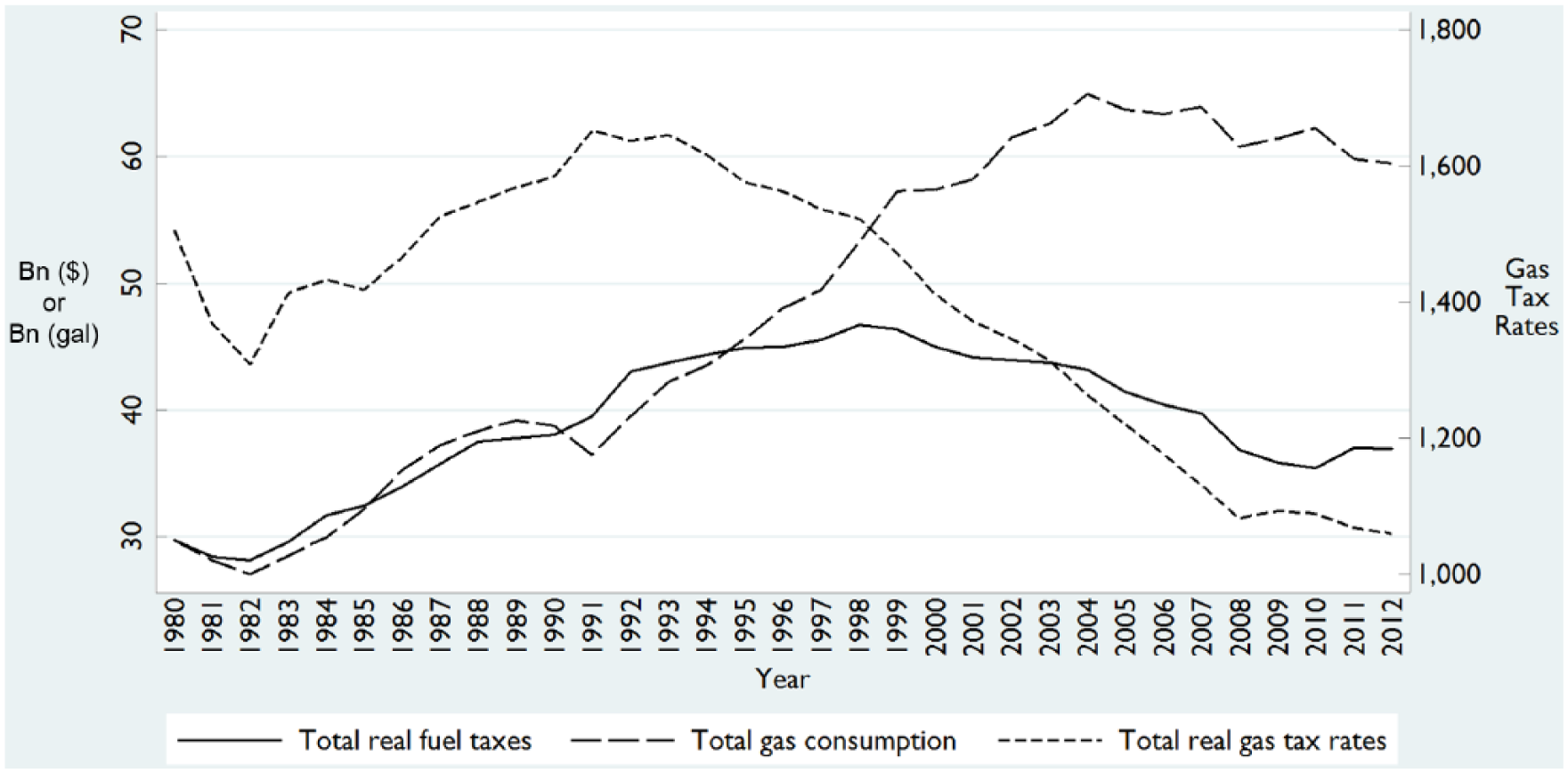
Fuel tax revenues, gasoline consumption, and gas tax rates for 48 contiguous states during 1980–2012.

Several studies have examined socially optimal gas tax rates, which take into account the negative externalities associated with driving (air pollution, traffic congestion, and accidents) and oil dependence (as in Lin and Prince 2009). For instance, Parry and Small (2005) conclude that the combined optimal fuel tax rates (both federal and state) in the United States should be about $1.01 per gallon, which was nearly double the highest federal and state rate of 57.4 cents per gallon in Connecticut in 1997. The current literature, however, has not settled on a revenue-maximizing gas tax rate. This paper seeks to answer this question by conducting a state-level analysis on a data panel of 48 contiguous states between 1980 and 2010. We find that states have considerable room to raise gas tax rates for higher transportation funds. However, as detailed in a series of supplementary analyses, the road to maximizing state fuel tax revenue can be bumpy, with countervailing forces resulting from tax-induced consumer behavior changes. We highlight these revenue-dampening countervailing effects that policy makers and planners should consider.

The paper proceeds as follows. The next section provides a background on state gas tax rates, followed by a review of related articles. We then present our empirical model and strategy and discuss our results. We finally conclude the paper with policy and planning implications from our empirical findings.

Background

State Gasoline Tax Rates

State gas taxes were first introduced in Oregon in February 1919 and quickly spread across the country. By 1924, gas taxes were in effect in 36 states (Martin 1924). Early gas tax rates started as low as 1 cent per gallon but have since increased considerably. Since 1960, the average nominal state-level gas excise tax has increased almost fourfold (O’Connell and Yusuf 2013). As of this analysis, Connecticut currently has the highest state gas tax rate of 39 cents per gallon with several states close behind.

Since 1966, there have been more than 500 (often incremental) changes to state-level gas excise taxes, which represents a change in the average state’s excise tax rate approximately once every four years (Li, Linn, and Muehlegger 2014). More than 90 percent of these state-year changes have been associated with a tax rate increase. Figure 2 shows that states vary in the frequency and size of their tax rate changes, and that five states (California, Connecticut, Pennsylvania, Rhode Island, and Washington) had the highest standard deviations in gas tax rates during the period 1980–2012.

Figure 2.

Gas Tax Rates by State during 1980–2012.

Much of this year-to-year variation can be attributed to the introduction of variable tax rates, which were popularized in the 1970s. A variable gas tax rate that can be adjusted every three to six months is generally indexed to one of several market indicators (e.g., the consumer price index, wholesale gas prices, and retail gas prices) and allows for a flexible yet rules-based response to changing market conditions. Unfortunately, even under a system of regular tax rate adjustments, state-level nominal excise gas tax rates have largely failed to keep pace with overall inflation. In fact, Bowman and Mikesell (1983) found that gas rate increases as a result of indexed rate adjustment during 1963–1983 were not larger than those from statutory change. Between 1980 and 2012, the average state-level nominal tax rate increased from nearly 10 cents to 22.3 cents per gallon. However, after adjusting for inflation, the average real tax rate actually decreased from nearly 10 cents per gallon in 1980 to 7 cents per gallon in 2012.

The national survey by Rall et al. (2011) shows that fuel tax revenues are used primarily for transportation purposes. Specifically, twenty-six states have constitutional or statutory provisions on earmarking fuel tax revenues exclusively for highway and road purposes. The remaining twenty-two lower states use fuel tax revenue principally for transportation purposes. In four contiguous states, state transportation funds including fuel taxes flow directly (without legislative appropriations) to state departments of transportation—the state’s leading agency in transportation planning activities. Many states also have explicit constitutional/statutory prohibitions on the diversion of fuel tax revenues for other nontransportation purposes. Nesbit and Kreft (2009) found that highway spending increased by nearly one dollar for every dollar of earmarked highway revenues, suggesting little diversion of earmarked gas tax dollars for other nontransportation purposes.

Excise gas tax rates are also levied at the federal and local levels. The federal excise gas tax rate was quite stable over time at 4, 9, 9.1, and 14.1 cents per gallon in 1980, 1983, 1987, and 1991, respectively. It increased to 18.4 in 1993 and remains so ever since. Unfortunately, these excise taxes are of limited use in local governments. Goldman, Corbett, and Wachs (2001) find in their comprehensive survey of local option transportation taxes that local gas taxes have been widely adopted in only four (Alabama, Florida, Illinois, and Nevada) of the thirteen contiguous states that currently authorize local option fuel taxes. Further, local gas tax rates are quite low (e.g., the median county fuel tax rate in Alabama in 2016 is 2 cents per gallon).

Related Studies

This review covers related studies in the extant literature (additional works will be discussed in supplementary analyses). In 1974, Arthur Laffer sketched a hypothesized relationship between tax rates and government revenues on a cocktail napkin. Under this concave continuous curve, tax revenue achieves a global maximum at a positive but less than 100 percent tax rate. The shape of this curve is driven by two competing effects, which Laffer termed “arithmetic” and “economic.” The arithmetic effect states that, holding all else constant, an increase in the tax rate will increase total revenue. In contrast, the economic effect recognizes that an increase in the tax rate will erode a portion of the tax base, muting (or even wholly negating) any tax revenue increase. At low tax rates, the arithmetic effect dominates and an incremental tax increase raises total revenue. As tax rates continue to rise, more and more of the underlying tax base is eroded, and total revenue eventually declines.

The Laffer curve has been the subject of considerable research since the early 1980s (e.g., Fullerton 1982). Although there have been a large number of studies on how government revenue responds to tax rate changes (e.g., Strulik and Trimborn 2012; Trabandt and Uhlig 2011), there has been relatively little work on the effect of state-level gas tax rates on state revenues. O’Connell and Yusuf (2013) concluded from a simulation analysis that a variable-rate gas tax structure based on indicators of need generates more revenues than a fixed-rate gas tax. An earlier study by Ang-Olson, Wachs, and Taylor (2000) concluded that states were experiencing a fiscal crisis because gas tax rates did not keep pace with inflation and suggested indexing the tax rates to the Consumer Price Index for revenues to be on par with inflation. In a rebuttal to Ang-Olson, Wachs, and Taylor (2000), Farkas (2000) argued that states were having “a steady, increasing, and sufficient flow of revenues” from gas taxes.

Recent studies have sought to determine the optimal gas tax taking into account negative driving externalities. Similar to Parry and Small (2005) discussed earlier, West and Williams (2007) estimated the optimal gas tax to be twice as large as the current level. Using Parry and Small’s (2005) model, Lin and Prince (2009) suggested that the optimal gas tax in California would be $1.37 per gallon, much higher than the 2010 excise gas tax rate of 35.3 cents (excluding the federal excise tax, and state and local sales taxes).

As long as the current gas tax rate is lower than the revenue-maximizing rate, raising tax rates constitutes a potential policy lever a state can tap to increase needed funding for transportation purposes. Although Uri and Boyd’s (1998) computable general equilibrium model produced positive results on production and consumption from a reduction in gas tax rates, later studies provided strong support for higher gas taxes. Wachs (2003) discussed a dozen reasons for raising gas taxes, including the fact that gas tax rates in the US were still low relative to other countries as well as to the past (due to inflation). Compared to fuel efficiency standards and other transportation fuel alternatives, Litman (2005) rated fuel tax increases as a more effective mechanism to accomplish policy-maker objectives such as energy conservation, emission and congestion reductions, traffic safety, and equity. In line with Litman, Karplus et al. (2013) showed that gas taxes are much less costly than fuel economy standards for new passenger vehicles to achieve the same level of emission reductions. Using expenditures, instead of annual income, as an indicator of household well-being, Poterba (1991) found the gas tax to be far less regressive than conventional analyses. Bento et al. (2009) showed that increases in the gas tax improved efficiency. Grabowski and Morrisey (2006) found that higher taxes saved lives. Specifically, they found that a 10 percent increase in the state gas tax was associated with a 0.6 percent decrease in the traffic fatality rate.

Empirical Model and Strategy

A state’s annual gas tax revenue is a function of its prevailing excise gas tax rate and the quantity of gas consumed. While state governments have no direct control over the market-determined equilibrium quantity consumed, gas tax rates act as a policy tool that can be used to raise additional revenue. Assuming a constant oil supply curve, a standard analysis of demand for gas indicates that quantity consumed changes with (1) retail or tax inclusive gas prices, represented as a movement along the demand curve, and (2) external factors, represented as a shift in the demand curve. Holding all outside factors constant, a tax rate change will increase total revenue when the resulting percentage increase in gas prices is greater than the percentage decrease in quantity consumed. This occurs when demand is relatively price-inelastic, which is empirically supported by recent studies (Brons et al. 2008). This price inelasticity leads to a higher pass-through rate of gas taxes to retail prices. Coyle, DeBacker, and Prisinzano (2012) find that 80 percent of fuel tax increases fall on consumers.⁴

This economic theory informs our empirical specification in which we model a state’s per capita fuel tax revenue (R) as a function of the state-level excise tax (T), the pre-tax price of gas (P), and a series of demand shifters (X₁ and X₂). Our estimating equation is specified as follows:

R_{s t} = γ_{s} + δ_{t} + θ_{1} T_{s t} + θ_{2} T_{s t}^{2} + ψ P_{s t} + β_{1} X_{1, s t - 1} + β_{2} X_{2, s t} + ε_{s t}

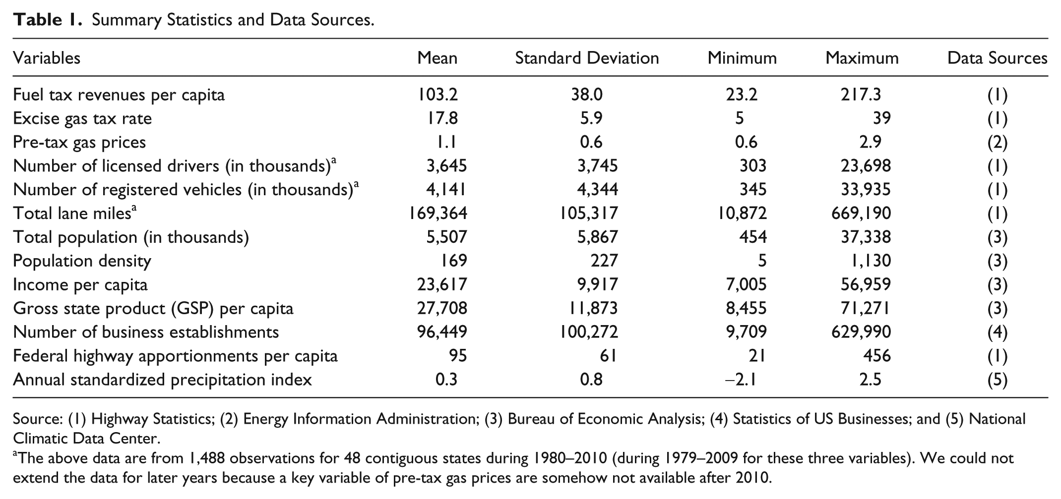
where s and t index states and years, respectively. State ﬁxed effects, $γ_{s}$ , control for time-invariant state-speciﬁc unobserved heterogeneity. These unobserved state-level factors can have both direct (e.g., local tax enforcement efforts) and indirect (e.g., demand shifters such as local topography, local option fuel taxes) effects on fuel tax revenue. Year fix effects, $δ_{t}$ , control for macro shocks to gas consumption across the states, which includes federal gas tax changes and technological advances leading to higher average vehicle fuel efficiency.

To estimate equation (1), we collected data primarily from Highway Statistics for our 1980–2010 sample period. Table 1 provides summary statistics for each of the included variables and their data source. Our key explanatory variable is the state-level excise gas tax rate (T), which is levied on a per gallon basis. We also control for the pre-tax price of gas (P), which excludes all federal, state, and local assessments, impacts consumer demand for fuel, and often partially informs the size of a state-mandated rate increase (Hajiamiri and Wachs 2010). T enters our specification as a quadratic to allow for nonlinear effects. Introducing this nonlinearity allows us to examine whether current gas tax rates are still to the left of the revenue-maximizing point of the Laffer curve.

Table 1.

Summary Statistics and Data Sources.

Variables	Mean	Standard Deviation	Minimum	Maximum	Data Sources
Fuel tax revenues per capita	103.2	38.0	23.2	217.3	(1)
Excise gas tax rate	17.8	5.9	5	39	(1)
Pre-tax gas prices	1.1	0.6	0.6	2.9	(2)
Number of licensed drivers (in thousands)^a	3,645	3,745	303	23,698	(1)
Number of registered vehicles (in thousands)^a	4,141	4,344	345	33,935	(1)
Total lane miles^a	169,364	105,317	10,872	669,190	(1)
Total population (in thousands)	5,507	5,867	454	37,338	(3)
Population density	169	227	5	1,130	(3)
Income per capita	23,617	9,917	7,005	56,959	(3)
Gross state product (GSP) per capita	27,708	11,873	8,455	71,271	(3)
Number of business establishments	96,449	100,272	9,709	629,990	(4)
Federal highway apportionments per capita	95	61	21	456	(1)
Annual standardized precipitation index	0.3	0.8	−2.1	2.5	(5)

Source: (1) Highway Statistics; (2) Energy Information Administration; (3) Bureau of Economic Analysis; (4) Statistics of US Businesses; and (5) National Climatic Data Center.

The above data are from 1,488 observations for 48 contiguous states during 1980–2010 (during 1979–2009 for these three variables). We could not extend the data for later years because a key variable of pre-tax gas prices are somehow not available after 2010.

The first group of demand shifters, X₁, include the total number of licensed drivers, yearly vehicle registrations (including automobiles, buses, and trucks), and highway lane miles. The number of licensed drivers and yearly vehicle registrations proxy for the number of motorists on the road, while highway lane miles provide a measure of road capacity. Because these variables may be affected by contemporaneous changes in fuel tax rates, they enter our specification with one-year lags.

The remaining controls are plausibly exogenous and enter our model unlagged as X₂. Demand for gasoline may change with economic activity in a state. We proxy for such activity using total income per capita, gross state product per capita, and number of business establishments. These economic variables are expected to be positively correlated with demand for gas consumption because they are often associated with additional road traffic. For instance, increases in income are linked to higher rates of car ownership (Varma and Sinha 1997). X₂ also includes population density. While a larger population is expected to have higher demand for gasoline (Hymel, Small, and Dender 2010), population density may be negatively correlated with fuel tax revenues. Low population density is usually coupled with less available public transit, which leads to more use of private vehicles and heavier gasoline consumption (Parry and Small 2005).

This vector of controls also includes federal apportionments per capita for state highways and a variable measuring precipitation. States’ willingness to raise gas tax rates and thus gas tax revenues are dependent on federal transportation fund transfers. The higher the transfers, the less willing states are to raise gas tax rates. Following Gamkhar (2003) and Nguyen-Hoang (2015), we use federal apportionments, rather than federal grant expenditures, for state highways because federal highway expenditures, given their reimbursement nature, are potentially endogenous in equation (1). A rainfall index allows us to capture the potential effects of weather conditions on travel and thus demand for gasoline. A greater proportion of commuters are more likely to drive to work instead of taking public transportation when it rains, impacting the extent of motor vehicle usage (Maze, Agarwai, and Burchett 2006). We therefore include the annual average Standardized Precipitation Index (SPI). The SPI indicates the number of standard deviations that the observed amount of precipitation deviates from its long-term mean. A zero index value indicates the median of the distribution of precipitation, while −3 and +3 represent extreme dry and wet spells, respectively.

Treatment for Endogeneity

State governments are likely to consider forecasts of fuel tax revenues for a proposed gas tax increase. As a result, changes in the state fuel excise tax are potentially endogenous.⁵ To account for this potential endogeneity, we instrument for our two tax rate variables (T and T²) using three plausibly exogenous variables and Fuller’s (1977) modified limited-information maximum likelihood (LIML) estimator.⁶

The three independent variables (IVs) we instrument for T and T² are (1) a binary indicator for the presence of any tax and expenditure limitations (TELs) on state budgets as used in Kioko and Martell (2012), (2) the share of wage and salary public employees who are union members, and (3) the share of members in the state House of Representatives who are Republicans (we code the third variable to be 0 for Nebraska, which has a unicameral and nonpartisan legislature). While fuel taxes are usually earmarked for transportation purposes, states can also spend general funds (income taxes, sales taxes, or lotteries) on state highways. State-level TELs may limit a state’s total taxes or income taxes (Mullins 2010), which potentially affects the amount of general funds available for transportation and thus the amount of fuel taxes to be raised. In response to the effects of TELs on the availability of general funds for transportation, states may need to raise gas tax rates to increase fuel tax revenue. In other words, TELs may affect the size and timing of gas tax rate increases.

Earlier studies, such as Marlow and Orzechowski (1996), have shown that the degree of public sector unionism affects the level and nature of state spending, which is at least partially financed through fuel taxes. Also, for states with a gas tax rate structure that is not tied to a price index, the gas tax rate remains fixed until legislation is passed to change it. The frequency of this legislation and the size of proposed rate increases are at least partially driven by the composition of the state government. This suggests that the share of members in the state House of Representatives who are Republicans is potentially correlated with the fuel tax rate.

Results

Main Results

Table 2 reports our main estimation results. Column 1 details coefficient estimates from an initial ordinary least squares (OLS) regression without state fixed effects. As illustrated, the coefficients attached to T and T² are equal to 0.084 and −0.0012, respectively. These estimates are statistically significant at the 1% level and, together, indicate an average revenue-maximizing fuel tax rate of 35 ( $= - 0.084 / (- 0.0012 \times 2))$ cents per gallon. These estimated coefficients are potentially biased because this regression fails to control for time-invariant unobserved factors such as state fuel tax enforcement efforts, physical land features, or average road grades. When we add state fixed effects to our OLS regression, the coefficient on T increases to 0.094 while the coefficient on T² remains unchanged. These estimates are presented in column 2 and indicate an optimal average state-level excise tax rate of 39.2 cents per gallon.

Table 2.

Main Results (Dependent Variable: Log Per Capital Fuel Tax Revenue).

Key Variable	(1)	(2)	(3)
State-level excise tax (T)	0.084*** (0.0039)	0.094*** (0.0035)	0.10*** (0.016)
State-level excise tax squared (T²)	−0.0012*** (0.000092)	−0.0012*** (0.000081)	−0.0012*** (0.00030)
Pre-tax gas price (P)	−0.45*** (0.080)	−0.17** (0.068)	−0.39*** (0.15)
Year fixed effects	Yes	Yes	Yes
State fixed effects	No	Yes	Yes
p-value of Hansen J statistic			0.65
Cragg-Donald Wald F statistic			7.08
Number of observations	1,488	1,488	1,488

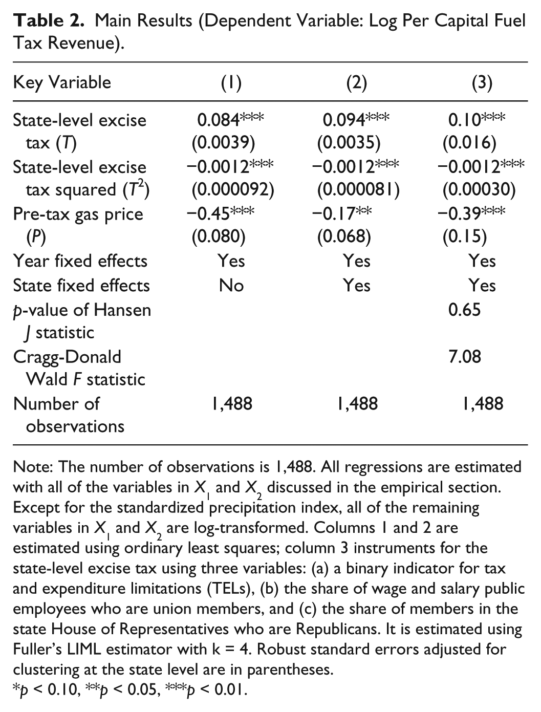
Note: The number of observations is 1,488. All regressions are estimated with all of the variables in X₁ and X₂ discussed in the empirical section. Except for the standardized precipitation index, all of the remaining variables in X₁ and X₂ are log-transformed. Columns 1 and 2 are estimated using ordinary least squares; column 3 instruments for the state-level excise tax using three variables: (a) a binary indicator for tax and expenditure limitations (TELs), (b) the share of wage and salary public employees who are union members, and (c) the share of members in the state House of Representatives who are Republicans. It is estimated using Fuller’s LIML estimator with k = 4. Robust standard errors adjusted for clustering at the state level are in parentheses.

p < 0.10, **p < 0.05, ***p < 0.01.

Because of endogeneity concerns, we next instrument for the state-level gas tax variables using the three IVs discussed earlier: a TEL indicator, the share of public employees who are union members, and the share of Republican members in the state House of Representatives. Column 3 details the resulting coefficient estimates that are calculated using Fuller’s modified limited-information maximum likelihood (LIML) estimator. The second panel of Table 2 reports the IV tests which show that the three IVs are exogenous of the estimated equation and strongly correlated with the two endogenous gas tax rate variables.⁷ As reported in column 3, the LIML model yields a slightly higher T coefficient of 0.1, while the coefficient attached to the quadratic term remains unchanged, –0.0012. Both coefficients are statistically significant at the 1% level and, together, indicate an average revenue-maximizing fuel tax rate of 41.7 cents per gallon. The fixed portion of state-level fuel excise taxes averaged 22.7 cents in 2010 with a range between 7.5 and 37.5 cents. Our results suggest that, as of 2010, all forty-eight contiguous states in the United States are on the upward sloping portion of the fuel tax Laffer curve and there is considerable room to raise gas tax rates in the future. As indicated in columns 1 through 3 of Table 2, as pre-tax gas prices increase, per capita fuel tax revenue decreases. This inverse relationship is to be expected given a downward sloping demand curve.

The qualitatively similar results between OLS and Fuller’s modified LIML suggest that failing to instrument for the fuel tax rate variables introduces only a minimal degree of bias. Because of the similarity of results, the following supplementary analyses are estimated using ordinary least squares.

Supplementary Analyses

There has been substantial scholarly interest in tax salience since the seminal work of Chetty, Looney, and Kroft (2009). In this study, the authors found that the demand for consumption goods declined when standard price tags were replaced with tax-inclusive (or more tax-salient) price tags. The study also found that a tax increase led to a larger decline in alcohol purchases when the tax increase was included in posted prices versus applied at the cash register. The evidence suggests that a more salient tax leads to a larger behavioral response than a similar but less salient tax. For the case of state gas tax rates, consumers potentially anchor to the previous year’s tax rate change and interpret subsequent tax rate increases through this lens. A fixed rate increase is potentially more salient if it represents a larger year-to-year percentage change in the tax rate. Following the tax salience literature, we hypothesize that the larger the annual percentage increase in gas taxes, the larger the behavioral response.

To capture this potential salience effect, we interact T with a variable indicating the associated year-on-year percentage change in the tax rate. A negative and significant coefficient on this interaction term is suggestive of a salience effect. For ease of interpretation, our auxiliary analyses are constrained to linear interaction effects. We attempted several higher order interactions including adding a quadratic term, but accounting for such second-order interaction effects had no economic significance on the results.

Column 1 of Table 3 reports the results of our salience analysis. The interaction between gas tax rates (T) and annual percentage change in T is negative and strongly significant. The coefficient attached to the interaction term suggests that consumers are more responsive to a gas tax change when it represents a year-on-year percentage increase. Holding the absolute size of any tax rate change constant, the larger the tax rate increase in percentage terms, the more elastic the consumer response. To put this effect into context, consider two states that each institute a 5-cent increase in fuel taxes, but start at different base rates. The base rate in state A is 15 cents and the base rate in state B is 20 cents. Calculations using the results of column 1 show that because of the perceived salience of the 33.3 percent tax rate increase in state A, its marginal effect on fuel tax revenue is muted by 11.3 percent (relative to the fuel tax revenue earned in the absence of the salience effect). In contrast, the 25 percent tax rate increase in state B only mutes potential fuel tax revenue by 8.7 percent.

Table 3.

Supplementary Analyses 1 (Interactions with Percentage Changes in Gas Tax Rates, Inflation, and Pre-tax Gas Prices).

	With Percentage Change in T	With Percentage Change in CPI	With Pre-tax Gas Prices
Key Variables	(1)	(2)	(3)	(4)	(5)
Gas excise tax rate (T)	0.10*** (0.0057)	0.10*** (0.0075)	0.094*** (0.0064)	0.094*** (0.0064)	0.094*** (0.0063)
T ²	−0.0014*** (0.00012)	−0.0014*** (0.00015)	−0.0014*** (0.00014)	−0.0013*** (0.00014)	−0.0014*** (0.00014)
T × Year-on-year percentage change in T	−0.0002*** (0.000027)
T × Year-on-year percentage change in CPI		−0.0013*** (0.00048)
T × P			0.0012(0.0013)		0.0017(0.0014)
T × Year-on-year percentage change in P				−0.00004* (0.000021)	−0.000055*** (0.000021)
Year-on-year percentage change in P				0.00041(0.00087)	0.00060(0.00086)
Log of total income per capita (Y)	0.47** (0.20)	0.42** (0.19)	0.43** (0.20)	0.41** (0.19)	0.43** (0.19)
Log of population density (D)	−0.20(0.14)	−0.15(0.14)	−0.15(0.15)	−0.17(0.15)	−0.15(0.15)
Pre-tax gas prices (P)	−0.15* (0.084)	−0.19** (0.085)	−0.19** (0.087)	−0.17(0.10)	−0.19* (0.100)

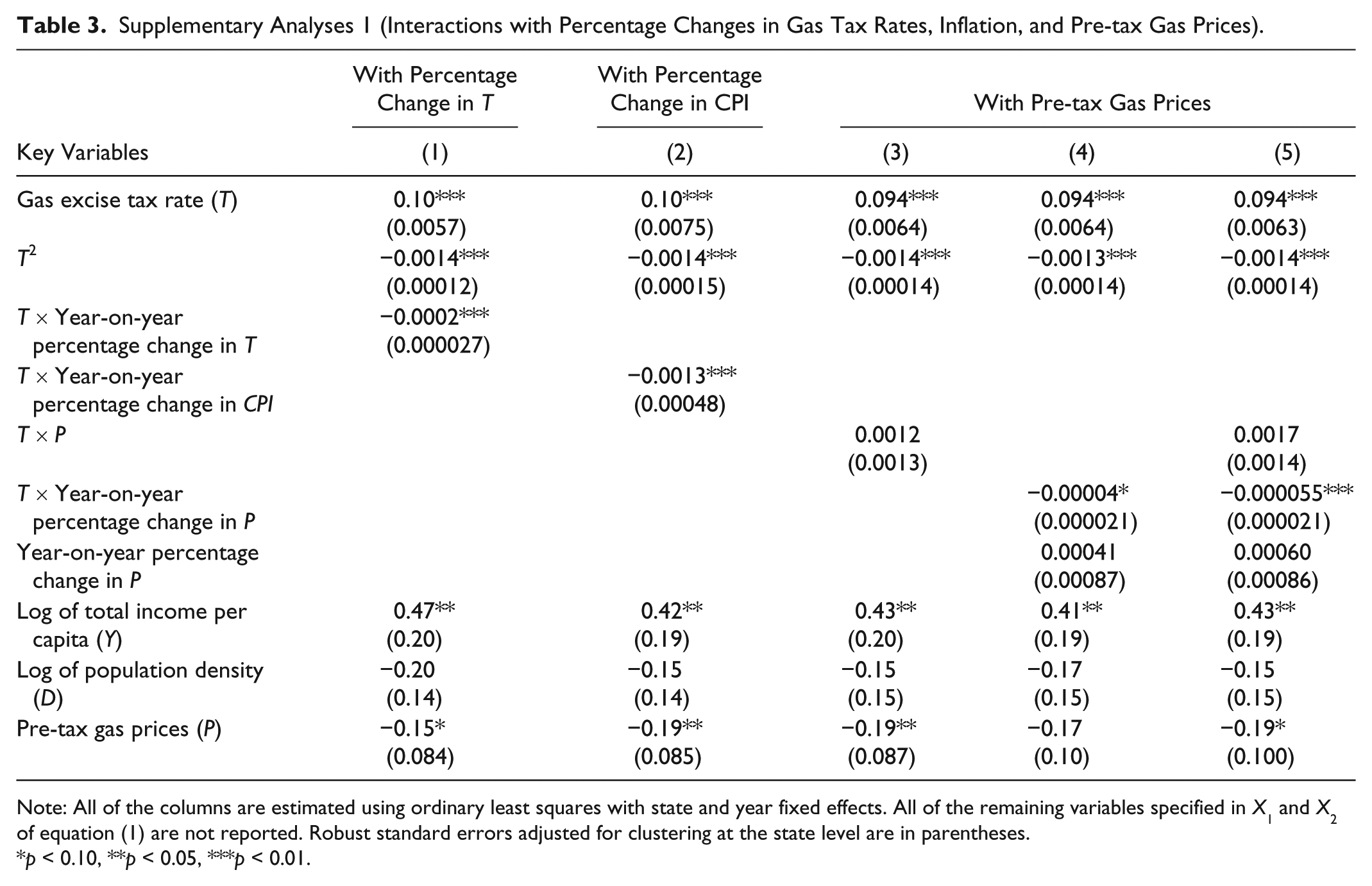
Note: All of the columns are estimated using ordinary least squares with state and year fixed effects. All of the remaining variables specified in X₁ and X₂ of equation (1) are not reported. Robust standard errors adjusted for clustering at the state level are in parentheses.

*p < 0.10, **p < 0.05, ***p < 0.01.

This seemingly irrational response could be a function of the media attention devoted to a given excise tax rate increase.⁸ A larger year-on-year percentage change may warrant wider media coverage, making the tax change more visible, and likely discouraging people from driving at the thought of having to pay more taxes. This explanation for a more pronounced consumer response from a larger percentage tax change is consistent with recent literature on the effects of tax salience on behavioral responses: a more salient tax change induces larger behavioral changes than a less salient change.

Next, we test for a differential consumer response across inflationary environments by interacting T with the year-on-year percentage change in the national consumer price index (CPI). Consumers may respond to gas tax rate increases in periods of high inflation in three ways: (1) if consumers suffer from money illusion and still think of currency in nominal terms, they may not moderate their response to a tax increase based upon the inflationary environment; (2) if they think about currency in real terms, they should be more responsive to a fixed tax rate increase during a period of low inflation than a period of high inflation; and (3) because of sticky wages, high inflation may temporarily erode consumer purchasing power (i.e., a leftward shift of a consumer’s budget constraint). In such a situation, an increase in gas tax rates may induce consumers to cut back on driving. We let the data inform which of these three effects ultimately dominate.

The results for the interaction effect of gas tax rates and inflation are reported in column 2 of Table 3. The coefficient of the interaction is negative and significant. This suggests that consumers do not think about gas tax rate increases alone in real terms, but rather that they see the purchasing power of their income eroded by inflation. Holding constant all else including nominal income, the purchasing power erosion appears to induce consumers to cut back on gasoline consumption, leading to a smaller revenue-enhancing effect of gas tax rate increases. To put this purchasing power effect in context, consider a fixed tax rate increase from 15 cents to 20 cents in two different inflationary periods. In period A, annual inflation grows at 3 percent (the US economy in 2004–2008), while in period B, annual inflation grows at 6 percent (the US economy in 1982 and 1990). The lower level of inflation in period A leads the fuel tax increase to result in 0.6 percent more tax revenue than in period B.

Our next auxiliary analysis is motivated by the findings of recent studies (Anderson, Kellogg, and Sallee 2013; Davis and Kilian 2011) that consumers respond differentially to changes in pre-tax gas prices versus gas tax rates. Of particular interest is how consumers moderate their response to a tax rate increase based on the pre-tax price of gas.

There is convincing empirical evidence that consumers are predominantly reference-dependent and use past (memory-based) and currently distributed (stimulus-based) prices as references for purchase decisions (Kalyanaram and Winer 1995). An increase in pre-tax gas prices measured in percentage terms, therefore, may allow us to capture reference-dependent consumer behavior. Stimulus-based consumers may use the total cost of gas as a reference for any increase in gas tax rates. Therefore, as pre-tax gas prices increase, these consumers will be less responsive to a fixed rate increase because it represents a smaller portion of the total gas price. Alternatively, consumers who use past gas prices as a reference and are sensitive to current changes (relative to past prices) would be more responsive to a concurrent increase in gas tax rates because it results in a larger change in retail prices. Under this memory-based reference mechanism, the larger the percentage change in pre-tax gas prices, the more responsive the consumers are to a simultaneous tax rate increase.

To explore these reference-dependent consumer behaviors, we use two specifications, one involving interactions between T and P and the other involving interactions between T and the year-on-year percentage change in P. Columns 3 to 5 of Table 3 report our results. While the coefficient on the interaction of T and P (T*P) is indistinguishable from zero in column 3, the interaction of T times annual percentage change in P (T*%∆P) is significant and negative in column 4. The coefficient on this interaction is qualitatively similar in column 5 when T*P and T*%∆P are included together as a robustness test. To put this result in context, we consider two otherwise identical states, A and B. Both increase their gas tax from 15 cents to 20 cents along with a 50-cent increase in the pre-tax price of gasoline from $1 to $1.50 in state A, and from $2 to $2.50 in state B. This pre-tax gas price increase mutes the effect of the associated fuel tax increase by 14.7 percent in state A, but by only 7.8 percent in state B. These results suggest that responses of memory-based consumers dominate those of stimulus-based consumers, which is consistent with Moon, Russell, and Duvvuri’s (2006) finding that memory-based consumers are more price sensitive.

Our final set of analyses attempt to capture evidence of differential consumer responses conditional on population density and per capita income. A higher population density is associated with an increase in the likelihood of switching from driving one’s own vehicle to other modes of commute such as public transit, carpooling, biking, or walking (Taylor and Fink 2013), which are often more conveniently available in densely populated areas. We include an interaction between T and population density to capture differential propensities for this switching behavior. The associated regression results are detailed in column 1 of Table 4 and show a negative and significant interaction between T and population density. To put this result in context, take two states, otherwise identical except for their respective population densities. Each state institutes a gas tax increase, raising the prevailing tax rate from 15 cents per gallon to 20 cents per gallon. Consumers in the denser state (characterized by a log population density of four) have more alternative transportation options, which allows for a more elastic response to the tax rate change. Alternatively, consumers in the more diffuse state (characterized by a log population density of two) have limited transport mode choice, which leads to a more inelastic demand for fuel. As a result of this differential response, the more diffuse state is able to raise an additional 6.7 percent in fuel tax revenue.

Table 4.

Supplementary Analyses 2 (Interactions with Population Density and Income).

Key Variables	With Population Density	With Income
Key Variables	(1)	(2)
Gas excise tax rate (T)	0.098*** (0.0052)	0.11*** (0.0077)
T ²	−0.0013*** (0.00012)	−0.0012*** (0.00015)
T×D	−0.0011** (0.00053)
T×Y		−0.0020*** (0.00071)
Log of total income per capita (Y)	0.39*** (0.15)	0.059*** (0.022)
Log of population density (D)	−0.047(0.084)	−0.25(0.16)
Pre-tax gas prices (P)	−0.17** (0.088)	−0.13(0.088)

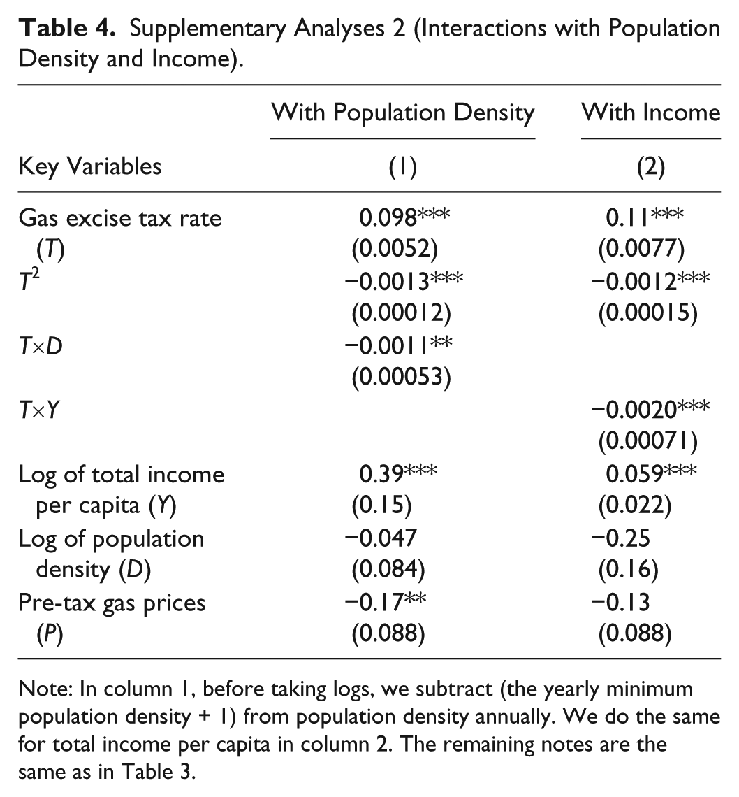
Note: In column 1, before taking logs, we subtract (the yearly minimum population density + 1) from population density annually. We do the same for total income per capita in column 2. The remaining notes are the same as in Table 3.

We next turn to the relationship between per capita income and the response to gas tax increases. There are two competing hypotheses. Higher-income households may be less sensitive to tax rate increases because fuel expenditures represent a smaller portion of the total household budget. Alternatively, studies have found that income is a significant factor in people’s willingness to pay the premiums associated with more fuel-efficient vehicles (Erdem, Şentürk, and Şimşek 2010). Faced with what may be perceived as a permanent tax rate increase, high-income households may be better equipped to live green by transitioning to more fuel-efficient vehicles, thereby driving down total fuel tax revenues. Column 2 of Table 4 documents the results when T is interacted with logged total income per capita (Y). The coefficient on this interaction is statistically significant and negative. This suggests that as income rises, consumers with higher ability to pay are more likely to switch to fuel-efficient vehicles in response to gas tax increases, putting a damper on fuel tax revenue growth.

To put this result in context, take two states that each increase excise tax rates from 15 cents per gallon to 20 cents per gallon, but are characterized by different levels of average wealth. Per capita income in state A is $35,000 while per capita income in state B is $45,000. While the wealthier state has a higher baseline level of fuel consumption, its households are also more likely to substitute into more fuel-efficient vehicles as a result of the tax rate increase (which is akin to an extensive margin response). This ultimately lowers revenues, and state A is able to raise 1.0 percent more in fuel tax revenue than state B.

Conclusions

State transportation funds are instrumental for transportation planning at not only the state but, in many cases, regional and local levels. The funds are also key for direct investments in surface transportation—a determinant of regional development. Unfortunately, while a substantial portion of American highways are in poor condition and in dire need of repair, many states are facing challenges in maintaining transportation expenditures (Pew Charitable Trusts 2014). Fuel taxes still represent a major revenue source for surface transportation expenditures, at least in the short run. The results from this study show that there is considerable room for states to increase gas tax rates before reaching an average revenue-maximizing gas tax rate of nearly 42 cents per gallon. However, we find that the road to reaching this fiscally optimal gas tax rate is bumpy with countervailing factors that may mute or undermine the revenue-enhancing capacity of gas tax hikes. For one, a higher percentage increase in gas tax rates induces a larger consumer response, holding constant a unit increase in gas tax rates. Suppose that either Louisiana or Texas, each with a 2014 gas tax rate of 20 cents per gallon, wanted to raise their tax rate by an additional 5 cents. Because of this relatively low base, the 5-cent increase represents a 25 percent rate hike. According to our analysis, the extent of this rate hike would mute the size of the corresponding fuel tax revenue increase by 8.7 percent. We argue that this revenue-dampening effect is a function of the perceived salience of the associated tax rate increase.

We also identify four other countervailing factors that may offset a revenue increase from a gas tax rate hike. First, raising gas taxes in a high inflationary environment is likely to mute any resulting increase in tax revenues. This happens when consumers who, given sticky wages, find their disposable income eroded and cut back on driving in response to gas tax hikes. Second, reference-dependent consumers who use past gas prices as an anchor may respond more (by driving less) to gas tax increases that occur in tandem with a rise in gas prices. Finally, increases in both state population (and thus in population density) and income per capita appear to mute the effect of gas tax increases on fuel tax revenues. This is due to consumers switching to alternative modes of transportation or more fuel-efficient vehicles in response to gas tax increases.

As found in a recent Gallup poll, two-thirds of Americans would vote against a state gas tax hike (Brown 2013). This significant level of voter opposition might be a reason for states’ past failed attempts to raise gas taxes (Watts, Frick, and Maddison 2012). However, several states have recently been successful at raising gas tax rates. In 2015, ten states enacted gas tax hikes from 3.5 cents as in Kentucky to 10 cents as in Iowa (Davis 2015). Several other states are still considering gas tax increases and are likely to join these ten states in the coming years.

Our study’s findings provide several implications for states that are considering raising gas taxes with minimal revenue-offsetting effects. First, states might adopt a gradual approach to raising tax rates, starting with a relatively small increase and then slowly moving to larger incremental changes. Second, states might try to time gas tax hikes during periods of low inflation or low pre-tax gas prices (e.g., the recent plunge in gas prices during late 2014 and early 2015). Third, although growth in population and income is desirable, states should take into account their interaction with gas tax increases when contemplating a gas tax increase. Finally, the ten states with gas tax hikes in 2015 benefited from the lowest average crude oil prices since 2009 (Breul 2016). Crude oil prices are forecast to continue to drop in 2016 before beginning to pick up gradually in 2017 (World Bank 2015). Other states considering gas tax increases should enact the increases as soon as possible before crude oil prices, and thus pre-tax gas prices, start to rise and potentially mute the revenue-generating effects of gas tax hikes.

This study provides implications for planning practitioners and researchers. Our findings suggest that the states with recent gas tax hikes can expect to see an increase in fuel tax revenue. This impending increase in fuel tax revenue raises multiple questions. First, will staff in state departments of transportation—states’ leading transportation planners—plan to spend the additional revenue on new construction projects, or on otherwise delayed maintenance and repair? Although it is still early at the time of this paper, our reading of states’ tax hike bills suggests that new revenue will be used mostly for maintenance and repair. For example, a 10-cent tax hike in 2015 was expected to raise $200 million for Iowa to fund long-delayed road and maintenance projects in the first year (Hanson 2015). Another 2015 gas tax increase of 6 cents in Nebraska was projected to generate 75 million dollars annually for “a multimillion-dollar backlog in road and bridge repair and construction” (Pluhacek 2015). Other questions include whether state departments of transportation might find it fiscally viable to provide additional financial incentives (or support) for more state–local coordination in transportation planning, or for the operations of local and regional transportation planning agencies. Practicing planners in states with recent tax hikes will soon be able to answer these questions for themselves. These questions are worth pursuing for planning researchers.

Footnotes

Declaration of Conflicting Interests

The author(s) declared no potential conflicts of interest with respect to the research, authorship, and/or publication of this article.

Funding

The author(s) received no financial support for the research, authorship, and/or publication of this article.

Notes

Author Biographies

Phuong Nguyen-Hoang is an assistant professor in the School of Urban and Regional Planning and Public Policy Center, both at the University of Iowa. His research revolves around public policy and finance, including education and transportation finance.

Alexander Bogin is a senior economist in the Capital Policy Branch at the Federal Housing Finance Agency (FHFA). Bogin has expertise in urban economics, applied econometrics, and financial modeling.

References

American Road & Transportation Builders Association. 2014. “Transportation FAQs.” goo.gl/RpLj3h.

American Society of Civil Engineers. 2013. 2013 Report card: Bridges. Reston, VA: American Society of Civil Engineers.

Anderson

S. T.

Kellogg

Sallee

J. M.

2013. “What Do Consumers Believe about Future Gasoline Prices?” Journal of Environmental Economics and Management 66 (3): 383–403.

Ang-Olson

Wachs

Taylor

B. D.

2000. “Variable State Gasoline Taxes.” Transportation Quarterly 54 (1): 55–58.

Bento

A. M.

Goulder

L. H.

Jacobsen

M. R.

von Haefen

R. H.

2009. “Distributional and Efficiency Impacts of Increased US Gasoline Taxes.” American Economic Review 99 (3): 667–99.

Bhatta

S. D.

Drennan

M. P.

2003. “The Economic Benefits of Public Investment in Transportation: A Review of Recent Literature.” Journal of Planning Education and Research 22 (3): 288–96.

Bowman

J. H.

Mikesell

J. L.

1983. “Recent Changes in State Gasoline Taxation: An Analysis of Structure and Rates.” National Tax Journal 36 (2): 163–82.

Breul

2016. Crude Oil Prices Started 2015 Relatively Low, Ended the Year Lower. Washington, DC: US Energy Information Administration. goo.gl/TAEeGk

Brons

Nijkamp

Pels

Rietveld

2008. “A Meta-analysis of the Price Elasticity of Gasoline Demand. A SUR Approach.” Energy Economics 30 (5): 2105–22.

10.

Brown

2013. “In U.S., Most Oppose State Gas Tax Hike to Fund Repairs.” Des Moines Register, April 22. goo.gl/r41DYp

11.

Chetty

Looney

Kroft

2009. “Salience and Taxation: Theory and Evidence.” American Economic Review 99 (4): 1145–77.

12.

Coyle

DeBacker

Prisinzano

2012. “Estimating the Supply and Demand of Gasoline Using Tax Data.” Energy Economics 34 (1): 195–200.

13.

Crabbe

A. E.

Hiatt

Poliwka

S. D.

Wachs

2005. Local Transportation Sales Taxes: California’s Experiment in Transportation Finance.” Public Budgeting & Finance 25 (3): 91–121.

14.

Davis

2015. “Sweet Sixteen: States Continue to Take on Gas Tax Reform.” Tax Justice Blog. goo.gl/S67RFU

15.

Davis

L. W.

Kilian

2011. “Estimating the Effect of a Gasoline Tax on Carbon Emissions.” Journal of Applied Econometrics 26 (7): 1187–1214.

16.

Erdem

Şentürk

Şimşek

2010. “Identifying the Factors Affecting the Willingness to Pay for Fuel-Efficient Vehicles in Turkey: A Case of Hybrids.” Energy Policy 38 (6): 3038–43.

17.

Farkas

Z. A.

2000. “Variable-Rate State Gasoline Taxes Revisited.” Transportation Quarterly 54 (3): 21–24.

18.

Fullerton

1982. “On the Possibility of an Inverse Relationship between Tax Rates and Government Revenues.” Journal of Public Economics 19 (1): 3–22.

19.

Fuller

W. A.

1977. “Some Properties of a Modification of the Limited Information Estimator.” Econometrica 45 (4): 939–54.

20.

Gamkhar

2003. “The Role of Federal Budget and Trust Fund Institutions in Measuring the Effect of Federal Highway Grants on State and Local Government Highway Expenditure.” Public Budgeting & Finance 23 (1): 1–21.

21.

Gauthier

H. L.

1970. “Geography, Transportation, and Regional Development.” Economic Geography 46 (4): 612–19.

22.

Goldman

Corbett

Wachs

2001. Local Option Transportation Taxes in the United States (Part One: Issues and Trends). Institute of Transportation Studies, University of California at Berkeley.

23.

Grabowski

D. C.

Morrisey

M. A.

2006. “Do Higher Gasoline Taxes Save Lives?” Economics Letters 90 (1): 51–55.

24.

Hahn

Hausman

Kuersteiner

2004. “Estimation with Weak Instruments: Accuracy of Higher-Order Bias and MSE Approximations.” Econometrics Journal 7 (1): 272–306.

25.

Hajiamiri

Wachs

2010. “Hybrid Electric Vehicles and Implications for Transportation Finance. Public Works Management & Policy 15 (2): 121–35.

26.

Hanley

Kuhl

2011. “National Evaluation of Mileage-Based Charges for Drivers.” Transportation Research Record 2221:10–18.

27.

Hannay

Wachs

2007. “Factors Influencing Support for Local Transportation Sales Tax Measures.” Transportation 34 (1): 17–35.

28.

Hanson

2015. “Iowa legislature approves 10-cent gas tax increase.” Iowa State Daily, February 24. goo.gl/HVYQmv

29.

Hymel

K. M.

Small

K. A.

Van Dender

2010. “Induced Demand and Rebound Effects in Road Transport.” Transportation Research Part B: Methodological 44 (10): 1220–41.

30.

Institute of Transportation Studies, and ICF Consulting. 2005. “Metropolitan-Level Transportation Funding Sources.” goo.gl/HxSLg9

31.

Junge

J. R.

Levinson

2012. “Financing Transportation with Land Value Taxes: Effects on Development Intensity.” Journal of Transport and Land Use 5 (1): 49–63.

32.

Kalyanaram

Winer

R. S.

1995. “Empirical Generalizations from Reference Price Research.” Marketing Science 14:G161–69.

33.

Karplus

V. J.

Paltsev

Babiker

Reilly

J. M.

2013. “Should a Vehicle Fuel Economy Standard Be Combined with an Economy-wide Greenhouse Gas Emissions Constraint? Implications for Energy and Climate Policy in the United States.” Energy Economics 36 (March): 322–33.

34.

Kioko

S. N.

Martell

C. R.

2012. “Impact of State-Level Tax and Expenditure Limits (TELs) on Government Revenues and Aid to Local Governments.” Public Finance Review 40 (6): 736–66.

35.

Laing

2015. South Dakota hikes gas tax. March 18. goo.gl/OAXJTS

36.

Linn

Muehlegger

2014. “Gasoline Taxes and Consumer Behavior.” American Economic Journal: Economic Policy 6 (4): 302–42.

37.

Lin

C.-Y. C.

Prince

2009. “The Optimal Gas Tax for California.” Energy Policy 37 (12): 5173–83.

38.

Lindblom

2015. “Lawmakers Release $16 Billion Transportation Plan with 11.9-Cent Gas Tax.” The Seattle Times, June 29. goo.gl/naEHRq

39.

Litman

2005. “Efficient Vehicles versus Efficient Transportation: Comparing Transportation Energy Conservation Strategies.” Transport Policy 12 (2): 121–29.

40.

Marlow

M. L.

Orzechowski

1996. “Public Sector Unions and Public Spending.” Public Choice 89 (1): 1–16.

41.

Martin

J. W.

1924. “The Administration of Gasoline Taxes in the United States.” National Municipal Review 13 (10): 587–600.

42.

Maze

Agarwai

Burchett

2006. “Whether Weather Matters to Traffic Demand, Traffic Safety, and Traffic Operations and Flow.” Transportation Research Record 1948 (January): 170–76.

43.

Moon

Russell

G. J.

Duvvuri

S. D.

2006. “Profiling the Reference Price Consumer.” Journal of Retailing 82 (1): 1–11.

44.

Mullins

D. R.

2010. “Fiscal Limitations on Local Choice: The Imposition and Effects of Local Government Tax and Expenditure Limitations.” In State and Local Fiscal Policy: Thinking Outside the Box?, edited by Wallace

, 201–65. Northampton, MA: Edward Elgar.

45.

Nesbit

T. M.

Kreft

S. F.

2009. “Federal Grants, Earmarked Revenues, and Budget Crowd-Out: State Highway Funding.” Public Budgeting & Finance 29 (2): 94–110.

46.

Nguyen-Hoang

2015. “Volatile Earmarked Revenues and State Highway Expenditures in the United States.” Transportation 42 (2): 237–56.

47.

Nguyen-Hoang

Yeung

2014. “Dollars for Lives: The Effect of Highway Capital Investments on Traffic Fatalities.” Journal of Safety Research 51: 109–15.

48.

O’Connell

Yusuf

J.-E.

2013. “Improving Revenue Adequacy by Indexing the Gas Tax to Indicators of Need a Simulation Analysis.” Public Works Management & Policy 18 (3): 229–43.

49.

Parry

I. W. H.

Small

K. A.

2005. “Does Britain or the United States Have the Right Gasoline Tax?” American Economic Review 95 (4): 1276–89.

50.

Petroski

2015. “Gas Tax Hike Takes Effect Sunday.” Des Moines Register, February 25. goo.gl/MlZDrb

51.

Pew Charitable Trusts. 2014. “Intergovernmental Challenges in Surface Transportation Funding.” http://www.pewtrusts.org/en/research-and-analysis/reports/2014/09/intergovernmental-challenges-in-surface-transportation-funding Pew Charitable Trusts.

52.

Pluhacek

2015. “Gas Tax Hike Gets Nebraska Lawmakers’ OK, Governor’s Veto.” Lincoln Journal Star, May 7. goo.gl/tvM7m2

53.

Poterba

J. M.

1991. “Is the Gasoline Tax Regressive?” In Tax Policy and the Economy, edited by Bradford

D. F.

, 145–64. Cambridge, MA: MIT Press.

54.

Rall

Wheet

Farber

N. J.

Reed

J. B.

2011. Transportation Governance and Finance: A 50-State Review of State Legislatures and Departments of Transportation. Washington, DC: National Conference of State Legislatures and AASHTO Center for Excellence in Project Finance.

55.

Reed

2009. “We Test the Tips.”Edmunds.com. goo.gl/evYiTt

56.

Small

K. A.

Van Dender

2007. “Fuel Efficiency and Motor Vehicle Travel: The Declining Rebound Effect.” Energy Journal 28 (1): 25–51.

57.

Straszheim

M. R.

1972. “Researching the Role of Transportation in Regional Development.” Land Economics 48 (3): 212–19.

58.

Strulik

Trimborn

2012. “Laffer Strikes Again: Dynamic Scoring of Capital Taxes.” European Economic Review 56 (6): 1180–99.

59.

Taylor

B. D.

1995. “Public Perceptions, Fiscal Realities, and Freeway Planning: The California Case.” Journal of the American Planning Association 61 (1): 43–56.

60.

Taylor

B. D.

2000. “When Finance Leads Planning Urban Planning, Highway Planning, and Metropolitan Freeways in California.” Journal of Planning Education and Research 20 (2): 196–214.

61.

Taylor

B. D.

Fink

C. N. Y.

2013. “Explaining Transit Ridership: What Has the Evidence Shown?” Transportation Letters 5 (1): 15–26.

62.

Trabandt

Uhlig

2011. “The Laffer Curve Revisited.” Journal of Monetary Economics 58 (4): 305–27.

63.

Upchurch

2006. “The Future of Highway and Transit Finance.” TR News. goo.gl/Bw7qkQ

64.

Uri

N. D.

Boyd

1998. “Aggregate Impacts of the Proposed Reduction in the Motor Fuels Excise Tax in the United States.” Energy Economics 20 (3): 309–23.

65.

Vanka

Handy

Kockelman

K. M.

2005. “State-Local Coordination in Managing Land Use and Transportation along State Highways.” Journal of Urban Planning and Development 131 (1): 10–18.

66.

Varma

Sinha

1997. “Long-Term Highway Revenue Forecasting for Indiana.” Transportation Research Record 1576 (January): 46–55.

67.

Wachs

2003. “A Dozen Reasons for Gasoline Taxes.” Public Works Management & Policy 7 (4): 235–42.

68.

Watts

R. A.

Frick

K. T.

Maddison

2012. “Policy Making, Incrementalism, and News Discourse Gasoline Tax Debates in Eight U.S. States.” Public Works Management & Policy 17 (3): 238–55.

69.

West

S. E.

Williams

R. C.

2007. “Optimal Taxation and Cross-Price Effects on Labor Supply: Estimates of the Optimal Gas Tax.” Journal of Public Economics 91 (3-4): 593–617.

70.

Winston

Langer

2006. “The Effect of Government Highway Spending on Road Users’ Congestion Costs.” Journal of Urban Economics 60 (3): 463–83.

71.

World Bank. 2015. “World Bank Commodities Price Forecast (Nominal US Dollars).” Washington, DC: World Bank. goo.gl/NxG0mh.

72.

Zhao

Guo

Coyle

Robinson

Munnich

2015. “Revisiting the Fuel Tax-Based Transportation Funding System in the United States.” Public Works Management & Policy 20 (2): 105–26.