Finance Commission transfers in India: An alternative approach to the devolution process

Abstract

The study aims to identify significant missing dimensions that can enhance the existing formula-based devolution by the Finance Commission in its objectives towards vertical and horizontal fiscal balance. Horizontal devolution of the central divisible pool by the Finance Commission has been so far undertaken on a formula-based approach. The Commission includes certain criteria in the devolution formula as a proxy to address the differences in revenue capacity, fiscal need, and the cost of providing public goods of the states to eliminate horizontal fiscal imbalances. However, the methodology has been strongly questioned in its inclusiveness, ability to address the inherent complexities and actual needs of different states. The paper attempts to address the plausibility of incorporating new dimensions in the devolution formula of the Finance Commission to making it a more effective instrument facilitating vertical and horizontal equity in the backdrop of the huge diversity among the recipient states. The empirical analysis highlights significant impact of five criteria on fiscal imbalance of the states; income distance, fiscal performance index, demographic performance, geographic disadvantage index and state energy and climate index, which justify their inclusion in the devolution formula.

Keywords

Finance Commission tax devolution efficiency equity fiscal capacity H H2 H21 H3 H7

Introduction

The mechanism of transfers from Centre to the states of India is very complex and characterized by multiple channels. Until abolition of Planning Commission, there were mainly three direct routes of flow of fund from Centre to the States: the statutory transfers that comprise of tax-sharing and grants-in-aids by the Finance Commission (FC), plan grants by the Planning Commission, and the discretionary grants by the Central Ministries. After abolition of the Planning Commission in 2014, there are two main channels of fiscal transfers to the States, the FC and Central Ministries. The FC transfers to the States include devolution of sharable Central taxes and general-purpose grants to fill the post devolution revenue deficit of the States and specific purpose grants. The matching grants for Centrally Sponsored Schemes (CSS) and other grants are routed through the Central ministries. The formula-based tax devolution accounts for nearly 80% (average) of total fiscal transfers by the FC and the remaining 20% comprises general and specific purpose grants.

Determining the methodology for formula-driven fiscal transfers in India’s federal system remains both complex and contentious. Changes in the devolution formula over time suggest that political considerations often outweigh economic rationale, leading to disagreements over the choice of criteria and their weights.^1,2 Moreover, the indicators and weights used in the formula are frequently criticized as subjective and lacking strong theoretical justification.³ Such subjectivity raises the possibility that important state-specific characteristics contributing to horizontal inequalities are not adequately captured. The existing formula is criticized for its inherent over-emphasis on population or ‘population bias’ that put certain states at an advantageous position.^4–7

Against this backdrop, this study explores the potential for incorporating additional dimensions into the FC’s devolution formula to improve its effectiveness in promoting vertical and horizontal equity across diverse Indian states. The theoretical methodology is tested using secondary data, and weights for each significant criterion are derived according to their relative importance. The study makes three main contributions to the literature. First, it operationalizes Sarma’s¹ net marginal benefit of federating (NMBF) framework through an empirical model of fiscal imbalance. Second, it proposes a data-driven approach to identify criteria for tax devolution and determine their relative weights. Third, it introduces additional dimensions such as geographic disadvantage and energy efficiency and climate performance that capture structural heterogeneity across Indian states and are not adequately reflected in existing FC formulas.

The initial section on fiscal devolution discusses the existing approaches and provides a comparative overview of other major federal systems across the globe. It is followed by a detailed discussion on the proposed alternative theoretical framework. We explain the empirical strategy and the proposed criteria to be incorporated in proposed devolution formula in the methodology section. The section on empirical findings presents and discusses the estimated results and explains the new devolution formula with relative weights for each criterion and shares of the individual states.

Fiscal devolution: A review of existing approaches

Fiscal transfers through the FC operate at two levels: vertical devolution, which determines the sharing of the divisible pool between the Union and the states, and horizontal devolution, which allocates the states’ share among individual states. Horizontal devolution has traditionally followed a formula-based approach, but its effectiveness in addressing the diverse fiscal needs and capacities of states has been widely debated. Subrahmanyam⁸ argued that the criteria used for fiscal transfers lack a clear analytical foundation, particularly given the existence of multiple transfer channels operating under different principles. Similarly, the use of numerous criteria in the devolution formula has been criticized for diluting the intended objectives of transfers verges the transfers from the desired goals.^3,9,10 Scholars have also noted that the determination of transfer volumes often relies on subjective judgements, particularly in the context of gap-filling grants.^11,12 Bajaj and Viswanathan¹³ further observed deviations between projected and actual state finances used in FC assessments. Although equity remains a central objective of transfers, gap-filling mechanisms have been criticized for encouraging fiscal profligacy among recipient states while discouraging fiscally prudent ones. Godbole¹⁴ also pointed out that successive FCs have shown limited innovation and have rarely evaluated the assumptions underlying previous transfer frameworks.

The FC employs several criteria in the devolution formula as proxies to address differences in fiscal capacity, expenditure needs, and the cost of providing public goods across states. Over successive Commissions, both the criteria and their weights have evolved. Indicators such as population and area represent fiscal needs, while income distance or inverse income aims to equalize fiscal capacity. Other criteria including backwardness indices, infrastructure, tax effort, and fiscal discipline have been introduced to capture cost disabilities and incentivize better fiscal performance. However, in many cases the final allocation under these criteria is implicitly weighted by absolute population, except for area and forest cover. Given that population itself already carries substantial weight in the formula, this practice tends to overemphasize population and may disproportionately favour larger states. Such methodological issues raise concerns about the consistency of efficiency-based criteria and highlight the need for greater transparency in the selection of criteria, their weights, and the methodology used in the devolution formula.^15–17 Recent research emphasizes the growing role of fiscal transfers in promoting broader policy objectives such as environmental sustainability and the Sustainable Development Goals through criteria like forest cover and social indicators and stress the need to strengthen the design of transfer formulas.^18–22

Comparative experience from other federal systems provides useful insights into the design of fiscal equalization and decentralized transfer mechanisms. Australia operates one of the most comprehensive systems of horizontal fiscal equalization through the Commonwealth Grants Commission, which evaluates differences in both revenue capacity and expenditure needs of states to ensure comparable levels of public service provision across jurisdictions.²³ Canada’s constitutionally mandated equalization programme primarily focuses on equalizing fiscal capacity across provinces using representative tax bases so that provinces can provide reasonably comparable public services at comparable tax rates.²⁴ Germany, in contrast, follows a multi-tiered fiscal equalization framework combining horizontal redistribution with vertical federal transfers, including the redistribution of VAT revenues. In most federations, comparative studies show that fiscal equalization mechanisms are central instruments for addressing horizontal fiscal disparities and supporting equitable public service delivery across decentralized jurisdictions.^25,26 In comparison, India’s FC relies on a formula-based approach where both the criteria and their weights evolve across successive commissions. The present study contributes to this literature by proposing an empirically grounded framework in which the criteria and their weights are derived from their estimated impact on fiscal imbalance across states.

The literature on fiscal federalism and intergovernmental transfers in India has extensively analysed the evolution of FC formulas and their implications for vertical and horizontal equity.^3,22,27–31 However, the existing studies largely assess the criteria from normative or institutional perspectives without empirically testing whether they explain variations in fiscal imbalance. Additionally the weights assigned to the criterion are typically based on deliberative judgement rather than empirical estimation. This study addresses this gap by proposing an empirical framework in which both the selection of criteria and their weights are derived from their estimated impact on fiscal imbalance across states.

Alternative mechanism for tax devolution: Theoretical framework

The criteria used by different FCs are intended to capture differences in fiscal capacity and expenditure needs arising from the socio-economic characteristics of states.³² Ideally, the inclusion of any criterion should be justified by its measurable impact on fiscal imbalance, and its relative weight should reflect the magnitude of that impact. Sarma^1,3 proposed an objective methodology for determining transfer criteria based on the concept of the net marginal benefit of federating (NMBF), defined as the difference between the fiscal costs of joining the federation and the benefits derived from it, such as economies of scale in public service provision and increased revenue potential. In this framework, the fiscal imbalance is measured as the revenue–expenditure gap excluding fiscal transfers which serves as a proxy for NMBF. Using panel analysis, Sarma^1,3 identified population, inverse per capita income, and poverty as significant determinants of fiscal imbalance and suggested that the weights assigned to transfer criteria should reflect their empirical impact on this imbalance. This approach was further elaborated in Federal Fiscal Relations in India: Imperatives for Restructuring, highlighting the need for a more objective and analytically grounded framework for both vertical and horizontal resource sharing.

Fiscal imbalance, defined as the difference between state expenditure and own-source revenue, reflects both vertical and horizontal imbalances.³³ Differences in net fiscal benefits across regions can lead to inefficiencies and inequities in public service provision and may influence migration decisions, as suggested by the Tiebout³⁴ hypothesis. Effective fiscal transfer mechanisms should therefore aim to equalize fiscal capacities, address expenditure needs, and reduce cost differentials to ensure comparable levels of public services across regions.²³ Building on this framework, the present study develops an empirical approach to identify the determinants of fiscal imbalance across states and derive transfer criteria and their weights based on their estimated impact on fiscal imbalance. Fiscal imbalance for state i at time t is defined as the gap between the expenditure requirement and the own-source revenue capacity of the state. It reflects the extent to which a state’s expenditures exceed its internally generated revenues, excluding intergovernmental transfers. In this study, fiscal imbalance is measured as,

{F I}_{i t} = 1 - \frac{R_{i t}}{E_{i t}}

(1)

where R_it represents the own-source revenue of state i in year t, and E_it denotes the total expenditure of the state. A higher value of FI_it indicates a larger fiscal gap, implying greater dependence on intergovernmental transfers to finance expenditure. The revenue generation of a State i at time t will depend upon certain set of factors such as the fiscal capacity (K_it) of the State, some certain State-specific factors (F_it), efficiency of the government in raising revenue (A_it), the environmental factors (M_it) and the random factors (u_it). The expenditure of the State i at time t will depend upon the fiscal need (N_it) of the State, the cost of providing public services (C_it), State-specific factors (G_it) that causes cost disability, efficiency of the government expenditure (A_it), and the random factors (v_it).

R_{i t} = f (K_{i t}, F_{i t}, A_{i t}, M_{i t}, u_{i t})

(2)

E_{i t} = f (N_{i t}, C_{i t}, G_{i t}, A_{i t}, v_{i t})

(3)

The fiscal imbalance of a State i at time t will be,

{F I}_{i t} = f (K_{i t}, F_{i t}, A_{i t}, M_{i t}, N_{i t}, C_{i t}, G_{i t}, e_{i t})

(4)

where A_it indicates the efficiency factors that will influence both revenue and expenditure of the States. The environmental factors assumed to impact the fiscal imbalances through the revenue function as it will represent the conservation of resources that in turn limits economic activity and thus revenue generation. The combined random effects will be indicated by e_it.

Two key issues arise in specifying the model. First is the measurement of fiscal imbalance. It can be expressed as the gap between total expenditure and own-source revenue of a state, or as a ratio of this gap to total expenditure. However, this gap reflects not only vertical fiscal imbalance but also horizontal disparities and state-specific characteristics.

Second is the specification of state-specific variables. Sarma^1,3 captured such factors through state fixed effects in a panel framework without explicitly including observable state characteristics. In contrast, the present study incorporates observable state-specific variables through the components F_it and G_it to examine their influence on fiscal imbalance, while unobserved effects are absorbed in the constant term. The model is estimated using cross-sectional analysis, and standardized regression coefficients are used to derive the weights of significant criteria. Along with criteria used in earlier FCs, additional variables identified from the literature are also included in the analysis.

Methodology and data source

Criterion to be tested: Rational and measurement

The criteria used to test the theoretical framework discussed in previous section corresponding to their underlying objectives are depicted in Figure 1. The primary objective of FC transfers is to enhance fiscal capacity of the states and GSDP per capita found to have direct impact on fiscal imbalance.^3,32 Therefore, from equity dimension, income distance is incorporated with some methodological changes. To represent cost disability and expenditure need of the states, two composite indexes of area and population are used. Considering the significance of rewarding efficiency of the states in mechanism of fiscal transfers, performance indexes of fiscal position, demographic management and efficacy in energy usage and environment and are included in the analysis.

Figure 1.

Proposed criteria for tax devolution. Source: Author’s illustration.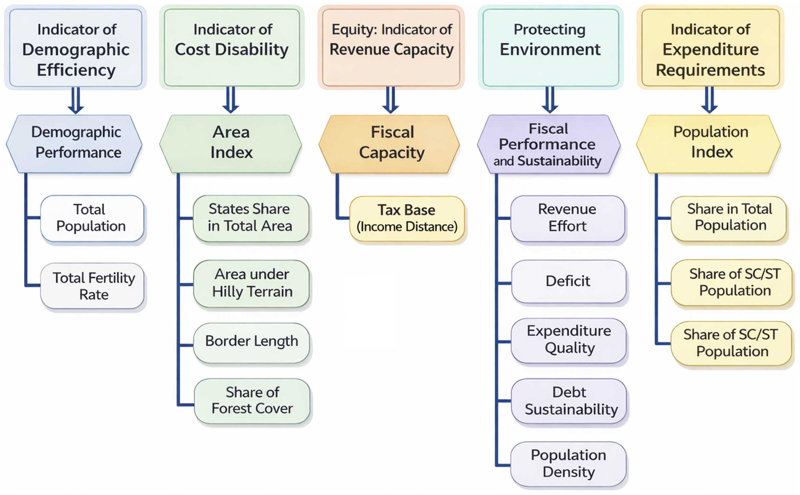

Demographic performance

Demography has a significant role in fiscal capacity and expenditure requirements of a state. The decision of the Fifteenth FC to use 2011 population created chaos and debate among the Southern States. This can also be justified as the southern states are putting continuous effort in population control. However, using outdated population of 1971 in deriving share of the states in tax devolution will also be technically incorrect and less representative of current situation. Therefore, the Fifteenth FC used demographic performance to reward states with low TFR. TFR itself significantly impacts fiscal imbalance of the states as found in previous analysis. Therefore, demographic performance is retained for the current analysis using same methodology and population of 2011. ${S i}^{D P}$ indicates share of state i under demographic performance criterion.

{S i}^{D P} = \frac{{D P}_{i}}{\sum {D P}_{i}}

(5)

where i = 1,2……n,

{D P = \frac{1}{{T F R}_{i}} \times P o p 2011}_{i}

{T F R}_{i} = 5 \times \sum_{15 - 19}^{45 - 49} {A S F R}_{i}

{A S F R}_{i} = \frac{N u m b e r o f l a s t y e a r s l i v e b i r t h i n t h e r e s p e c t i v e a g e g r o u p}{T o t a l f e m a l e p o p u l a t i o n i n t h e a g e g r o u p}

where

{D P}_{i}

= demographic performance of the i^th State.

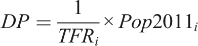
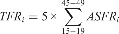
DP_i represents demographic performance index for state i which captures the relative performance of states in population stabilization, TFR_i indicates total fertility rate of the i^th State and ASFR_i age specific fertility rate of the i^th State. The indicator of demographic performance is constructed using the Total Fertility Rate (TFR¹) as an indicator of demographic transition.

Income distance

It is well established that income distance has valid foundation, solid methodology and strong redistributive properties along with incorporation of certain state-specific characters. We use income distance with similar methodology as given by the FCs, with certain modifications. Instead of using population weighted distance which favours states with larger population, distance from per capita income is used so that the redistributive aspects of the criteria are retained without any possible biasedness. We do not entirely nullify the requirement of states with larger population. Instead, we argue that population is already given its due weightage with a separate criterion by previous commissions, and for the present analysis, if population empirically shows significant impact on fiscal imbalance, it will be included in devolution formula.

{S i}^{I D} = \frac{({P C I}_{h} - {P C I}_{i})}{\sum ({P C I}_{h} - {P C I}_{i})}

(6)

i = 1,2……n,

{P C I}_{h}

= Per capita income of highest income State,

{P C I}_{i}

= Per capita income of i^th State.

${S i}^{I D}$ indicates share of state i under demographic performance criterion. To keep comparability intact, income distance is calculated from Haryana, though Goa and Sikkim have higher per capita income. These three states are given same distance as the state with fourth higher per capita GSDP, that is, Kerala. The final share of the state under income distance criterion is obtained directly from income distance. For calculation of income distance average per capita GSDP of 2016-19 is used.

Fiscal Performance Index (FPI)

For The composite FPI is constructed using the methodology employed by UNDP in computing the Human Development Index (HDI). A composite indicator helps summarize the overall fiscal performance of states in a single measure, which is useful for assessing fiscal prudence.³⁵ In this study, the FPI is computed incorporating five dimensions; deficit, own revenue effort, self-sufficiency, expenditure quality, and debt sustainability which are further divided into 11 indicators (details in Appendix). Each indicator is first converted into an index using the relative distance method to ensure comparability. Indicators representing improvement in fiscal performance are normalized with reference to the minimum value, while those indicating deterioration are normalized with reference to the maximum value, ensuring that higher index values consistently reflect better performance. The composite index is then derived using the geometric mean, which prevents high performance in one dimension from offsetting poor performance in another dimension.

Geographic Disadvantage Index (GDI)

There is a strong relationship between the geographical characteristics of a state and its fiscal imbalance. States with hilly terrain, particularly those with long international borders in addition to other geographical constraints, tend to experience higher fiscal imbalances.³⁶ Although previous FCs attempted to capture cost disabilities by assigning weight to area, this measure alone does not adequately reflect the challenges faced by states with difficult terrain or border-related constraints. To address this limitation, a GDI is constructed incorporating indicators such as the share of hilly terrain, border length, forest cover relative to the total area of the state, and the share of the state’s area in the total area of all states.

G D I_{i} = \frac{\sum X_{i}}{N}, i = 1, 2 . . 4

(7)

where X_i are sub-indices of cost disability as mentioned above. The index is constructed using the same methodology as the FPI. Each indicator is first normalized using the relative distance method to ensure comparability across states. After normalization, the final GDI is obtained as the average of the four sub-indices.

Population index

Population has had its dominance on the devolution formula for being a benchmark with equal per capita devolution. However, it needs to be highlighted that population density and share of scheduled caste and scheduled tribe population on fiscal imbalance of a state. Population index is prepared for the purpose of current analysis using normalized sub-indices of share of the states in total population, population density and share of SC/ST population. The final population index (PI) is obtained by taking average of the three sub-indices.

P I_{i} = \frac{\sum Z i}{N}

(8)

where Z_i are the sub-indices as discussed.

State Energy and Climate Index (SECI)

The State Energy and Climate Index (SECI) used in the analysis is adopted from the composite index developed by NITI Aayog to assess the performance of Indian states in energy efficiency, sustainability, and climate governance.³⁷ As a representative of all these aspects the State Energy and Climate Index is prepared by NITI Aayog using six dimensions and twenty-seven sub-indicators for 2019-20. The key dimensions are performance of DISCOMs (40% weight); access, affordability, and reliability of energy consumption (15% weight); clean and renewable energy initiatives (15% weight); efficiency in energy in terms of energy intensity of GSDP and energy saving (6% weight); environmental sustainability (12% weight); and innovation in the energy sector (12% weight). These dimensions collectively incorporate several indicators that capture different aspects of energy and climate performance of the states. In the present study, the composite SECI score reported by NITI Aayog is used directly rather than reconstructing the index, in order to maintain methodological consistency with the official framework and avoid additional measurement bias. Since the detailed construction of the index involves numerous sub-indicators, the full methodology is documented in the original NITI Aayog report, which is cited here, while only the composite score is used in the empirical analysis.

Estimation strategy

The empirical analysis incorporates six indicators i. e. income distance, GDI, FPI, SECI, demographic performance and, population index. The study employs secondary data obtained from RBI: A Study of State Finances (various issues), the RBI Handbook of Statistics on Indian Economy, the Ministry of Statistics and Programme Implementation, the Census of India (2011), and NITI Aayog. Cross-sectional data for 28 Indian states covering 2016–17 to 2018–19 are used, and a 3-year average is employed in the regression to smooth annual volatility in fiscal indicators and obtain more stable estimates of inter-state differences. A cross-sectional regression framework is adopted because the analysis focuses on structural variations in fiscal imbalance across states, rather than short-term fluctuations. Averaging over multiple years is commonly used in empirical public finance studies to minimize distortions from temporary fiscal shocks and to better capture the underlying fiscal characteristics of states and their relationship with fiscal imbalance.^38,39 Moreover, the key explanatory variables particularly GDI, FPI sub-indices, and SECI are themselves structural in character and do not vary significantly year-to-year. Treating them as time-varying panel variables would be methodologically inappropriate and would impose false precision on essentially time-invariant characteristics.

{F I}_{i} = α + β_{1} {I n c o m e D i s t a n c e}_{i} + β_{2} {D e m o}_{i} + β_{3} {F P I}_{i} + β_{4} {G D I}_{i} + β_{5} {S E C I}_{i} + β_{6} {P I}_{i} + u_{i}

(9)

Income distance and the GDI are expected to have positive coefficients, as lower income indicates weaker fiscal capacity and difficult terrain increases the cost of providing public services. The coefficients of fiscal performance, demographic performance, and the State Energy and Climate Index are expected to be negative, since better fiscal, demographic, and environmental management reduces fiscal imbalances across states. The population index is expected to be positive, as larger populations raise the demand for public goods and the resources required to finance them.

As the explanatory variables are measured in different units, the estimated coefficients from the original regression are not directly comparable. To address this issue, the variables are standardized and a standardized regression is estimated. The standardized coefficients (beta weights) measure the change in the dependent variable resulting from a one standard deviation change in each explanatory variable, thereby providing a scale-free measure of relative importance.^40,41

{Weight}_{i} = \frac{| β_{i} |}{\sum | β_{i} |}

(10)

where Weight_i indicates weight for each criterion,

β_{i}

represents standardized coefficients of each explanatory variable. These standardized coefficients are then used to derive the relative weights of the criteria in the proposed devolution formula, following the approach commonly used in the construction of composite indicators.^42–46

Empirical findings

Determinants of fiscal imbalance

Table 1 presents the correlation coefficients between the explanatory variables² and the fiscal imbalance. All independent variables included in equation (9) show a statistically significant association with fiscal imbalance across states. The coefficients are negative for the efficiency-based indicators, namely the SECI, demographic performance, and the FPI, indicating that higher efficiency in these areas is associated with lower fiscal imbalance. In contrast, variables representing fiscal capacity, expenditure needs, and cost disabilities, such as income distance, the GDI, and the population index, exhibit a positive correlation with fiscal imbalance. The relationships observed in the correlation analysis are also reflected in the scatter plots with fitted linear trend lines for each explanatory variable, which show patterns consistent with the correlation results (Figure 2).

Table 1.

Correlation with fiscal imbalance.

Variable	Correlation coefficient
SECI	−0.70***
Income distance	0.56***
Demographic performance	−0.62***
FPI	−0.62***
GDI	0.67***
Population index	0.46***

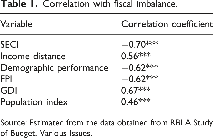
Source: Estimated from the data obtained from RBI A Study of Budget, Various Issues.

Figure 2.

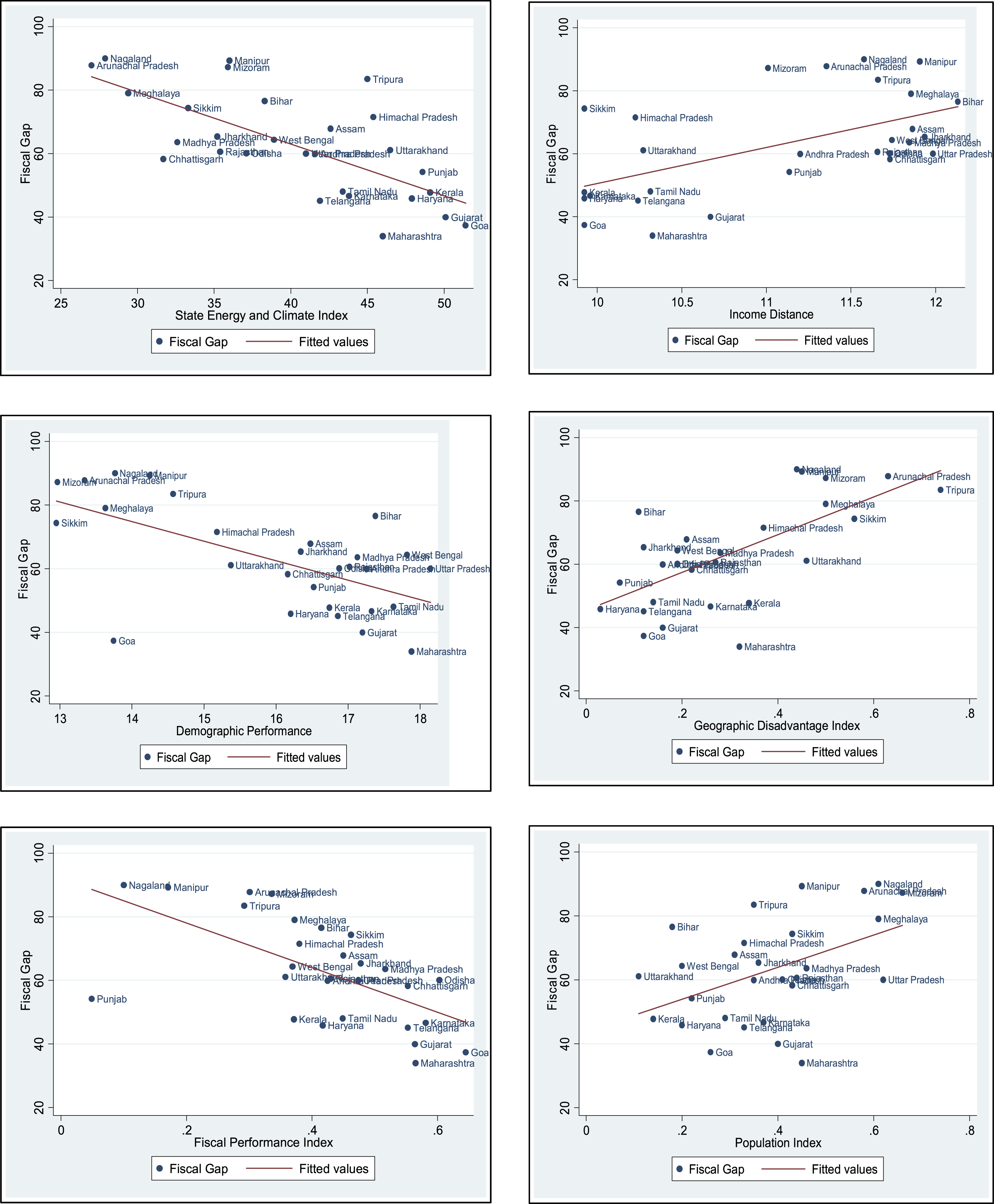
Scatter plot of each criterion against fiscal gap. Source: Author’s illustration.

The results of the cross-sectional regression analysis (equation (9)) for 28 Indian states are presented in Table 2. The Breusch-Pagan and Cook-Weisberg tests indicate the presence of heteroscedasticity; therefore, White’s heteroscedasticity-consistent standard errors are employed. The results of the multicollinearity test are reported in Table 3.

Table 2.

Result of cross-section regression.

Dependent variable: Fiscal imbalance
Explanatory variables	Coef.	Std. Error
SECI	−0.61**	0.24
Income distance	8.06***	1.78
Demographic performance	−3.02**	1.30
FPI	−28.41**	11.30
GDI	25.56***	8.43
Population index	−12.81	12.88
Constant	55.53***	19.10
F statistic	56.15***
R²	0.88

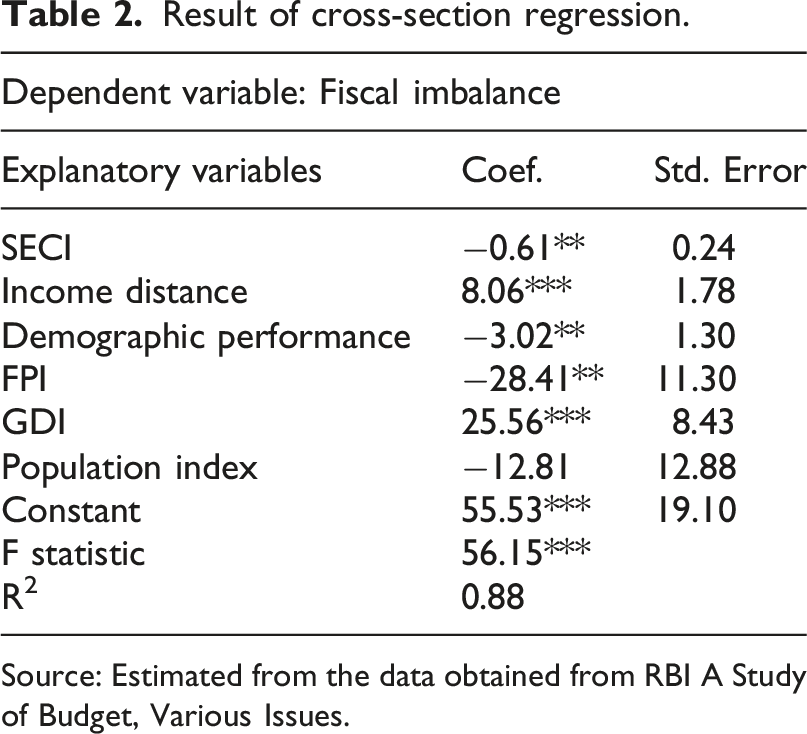
Source: Estimated from the data obtained from RBI A Study of Budget, Various Issues.

Table 3.

Results of standardized regression.

Dependent variable: Fiscal imbalance
Explanatory variables	Coef.	Std.
SECI	−0.26**	0.10
Income distance	0.40***	0.09
Demographic performance	−0.30**	0.13
FPI	−0.26**	0.10
GDI	0.28***	0.09
Population index	−0.11	0.12
Constant	0.01	0.07
F statistic	56.15***
R²	0.88

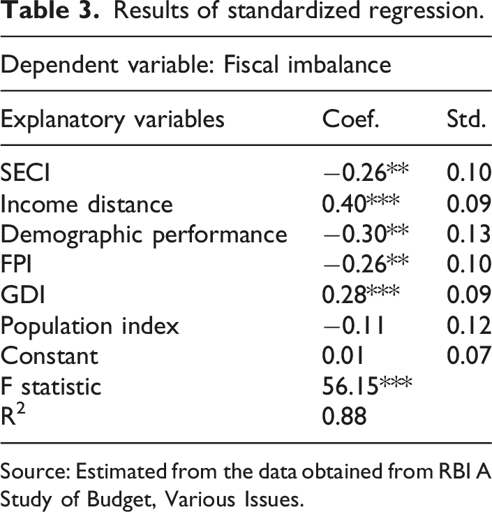
Source: Estimated from the data obtained from RBI A Study of Budget, Various Issues.

The State Energy and Climate Index is statistically significant at the five percent level and shows a negative relationship with fiscal imbalance across states. This suggests that more efficient use of energy is associated with lower fiscal imbalance. Improvements in energy efficiency can reduce the operational costs of governments through the adoption of energy-saving measures. Incorporating a criterion related to energy efficiency and climate initiatives may therefore provide states with additional incentives to improve their performance in these areas. Such incentives are particularly important as prudent energy management can help ease fiscal pressures on state governments. At the same time, improving energy efficiency and financing clean energy transitions remain significant challenges for Indian states and are closely linked to their fiscal management.⁴⁷

The FPI also exhibits a significant negative impact on fiscal imbalance. This indicates that states undertaking revenue-augmenting measures alongside prudent management of deficits, debt, and expenditure are likely to experience lower fiscal imbalance. Rather than rewarding revenue effort alone, recognition of overall fiscal performance may encourage states to strengthen their broader fiscal position. The inclusion of the FPI in the devolution formula may also help offset potential moral hazard arising from transfer dependence, excessive expenditure, and soft budget constraints associated with borrowing autonomy.

Demographic performance is significant at the five percent and shows a negative association with fiscal imbalance. The theoretical and empirical literature does not provide a clear consensus on the fiscal effects of demographic change, particularly in relation to declining fertility rates and their interaction with economic growth. The fiscal and growth implications of lower fertility are often country-specific and depend on the socio-economic characteristics of the region. In several European economies, lower fertility may lead to higher per capita income in the short run, although it may generate long-term challenges through reduced labour force participation and rising dependency ratios.⁴⁸ In the case of India, however, population control remains an important policy concern, especially as the country is expected to become the most populous nation, surpassing China. Empirical evidence suggests that lower fertility rates in India are positively associated with higher per capita income.⁴⁹ Rewarding improvements in demographic management may therefore yield positive fiscal outcomes, as reflected in the negative relationship with fiscal imbalance.

As expected, income distance and the GDI significantly increase fiscal imbalance. Income distance measures the gap between a state’s per capita income and that of the state with the highest per capita income, thereby reflecting relative differences in revenue capacity across states. Greater disparities in per capita income tend to widen fiscal imbalances. Recognizing these disparities, previous FCs have assigned substantial weight to income distance in the devolution formula. The empirical results support its effectiveness in capturing variations in fiscal capacity among states. Similarly, Geographic disadvantages also contribute to higher fiscal imbalance. States with difficult terrain face constraints on economic activity and often incur higher costs in delivering public services due to limited infrastructure and accessibility. The positive coefficient of the GDI confirms the fiscal implications of these structural constraints. Although area has been used by previous FCs as an indicator of the cost of providing public services, it does not fully capture all geographic challenges faced by states. Finally, although the population index was expected to have a significant effect on fiscal imbalance, the regression results do not provide statistical evidence supporting this relationship.

Inter-state variation across key devolution criteria

Indian states continue to display significant development imbalances that stem from their diverse socio-economic and geographical characteristics. States with the highest levels of per capita income include Goa, Sikkim, Haryana, Kerala, and Karnataka, whereas poorer states continue to struggle with a limited revenue base and weaker fiscal capacity. The largest income gaps relative to Haryana are observed in Bihar, Uttar Pradesh, Jharkhand, Manipur, and Assam. These disparities are further reinforced by rural–urban inequality. Income gaps between rural and urban areas in India have widened over time,⁵⁰ and many of the poorer states remain characterized by low levels of urbanization, with more than 70% of their population residing in rural areas. Such structural differences in urbanization significantly influence the fiscal capacity of states.

Demographic transition also plays an important role in shaping fiscal outcomes. India’s population growth, which has recently surpassed that of China, poses challenges for development, particularly because population growth remains concentrated in economically weaker states with limited fiscal capacity. States such as Meghalaya, Bihar, Uttar Pradesh, and Jharkhand continue to record relatively high total fertility rates (TFR) of 3.63, 2.93, 2.61, and 2.61, respectively. In this context, incorporating a criterion that rewards demographic performance through lower fertility rates becomes relevant both for encouraging demographic transition in lagging states and for recognizing the achievements of states such as Kerala, Karnataka, and Tamil Nadu that have successfully reduced fertility levels.

Geographical conditions also contribute to differences in fiscal outcomes across states. In terms of the GDI, Arunachal Pradesh records the highest share of forest cover relative to its area, followed by Tripura, while Haryana and Rajasthan have the lowest shares. With respect to international border length relative to state area, Tripura records the highest value. States with extensive hilly terrain are largely concentrated in the North-Eastern (NE) region, along with Himachal Pradesh and Uttarakhand (details in Appendix Table A1). Apart from their relative isolation from mainland India, the NE states face substantial terrain-related challenges, reflected in the larger shares of hilly terrain, forest cover, and international borders.

Fiscal performance across states is captured through the FPI, which combines five sub-indices reflecting different dimensions of state finances. Goa (0.65), Odisha (0.60), Karnataka (0.58), Maharashtra (0.56), and Gujarat (0.56) emerge as the top performers in overall fiscal performance (details in Appendix Table A2). These states generally perform well across most fiscal dimensions, although performance under the deficit index remains relatively weak for several states. Differences between high-income and low-income states are particularly evident in the own revenue effort index. Poorer and geographically disadvantaged states such as Bihar, Arunachal Pradesh, Manipur, and Nagaland exhibit persistently low revenue effort. A similar pattern is observed in the self-sufficiency index, where states with lower revenue effort remain more dependent on fiscal transfers. In contrast, states such as Haryana and Goa display relatively high levels of fiscal self-reliance. The lowest FPI scores are recorded for Punjab (0.05), Nagaland (0.10), Manipur (0.17), Tripura (0.29), and Arunachal Pradesh (0.30), with Punjab showing particularly weak performance across most dimensions except self-sufficiency. NE states generally combine low revenue effort with high dependence on fiscal transfers. Some states, including Punjab and Kerala, perform relatively well in self-sufficiency but show weaker outcomes in expenditure quality. Since the primary responsibility of governments is the provision of quality public services, efficient expenditure management becomes crucial for fiscal consolidation. Interestingly, states such as Madhya Pradesh, Jharkhand, and Arunachal Pradesh perform comparatively better in expenditure quality despite lower revenue effort and self-sufficiency. Debt sustainability also remains a concern across many states, as reflected in only moderate scores under the debt sustainability index.

Fiscal performance is also closely linked with environmental sustainability and energy efficiency. As the sixth-largest economy and home to nearly 17% of the global population, India faces rapidly growing energy demand, much of which continues to be met through conventional energy sources. Figure 3 presents the State Energy and Climate Index (SECI) scores reported in NITI Aayog’s State Energy and Climate Index Round-I. States are classified into three categories: front-runners (scores above 46), achievers (scores between 36 and 46), and aspirants (scores below 36), with the all-India average score recorded at 40.6. Across individual dimensions, Punjab records the highest score in DISCOM performance (77.1), Kerala leads in access, affordability, and reliability (67.3), Goa ranks highest in clean energy initiatives (62.4), Tamil Nadu performs best in energy efficiency (85.4), Sikkim leads in environmental sustainability (52.2), and Tripura performs best in new initiatives (58.7). In terms of overall SECI scores, Goa (51.4) ranks highest among small states, while Gujarat (50.1) leads among large states. Other states among the front-runners include Kerala, Punjab, Haryana, Uttarakhand, and Maharashtra. Despite these achievements, considerable scope for improvement remains, particularly in areas such as clean energy initiatives, environmental sustainability, and energy efficiency. Many aspirant states continue to perform poorly across these dimensions and also face challenges in ensuring reliable and affordable energy access. Arunachal Pradesh records the lowest overall SECI score, followed by Nagaland and Meghalaya.

Figure 3.

State-wise State Energy and Climate Index (SECI). Source: State Energy and Climate Index: Round-I, NITI Aayog.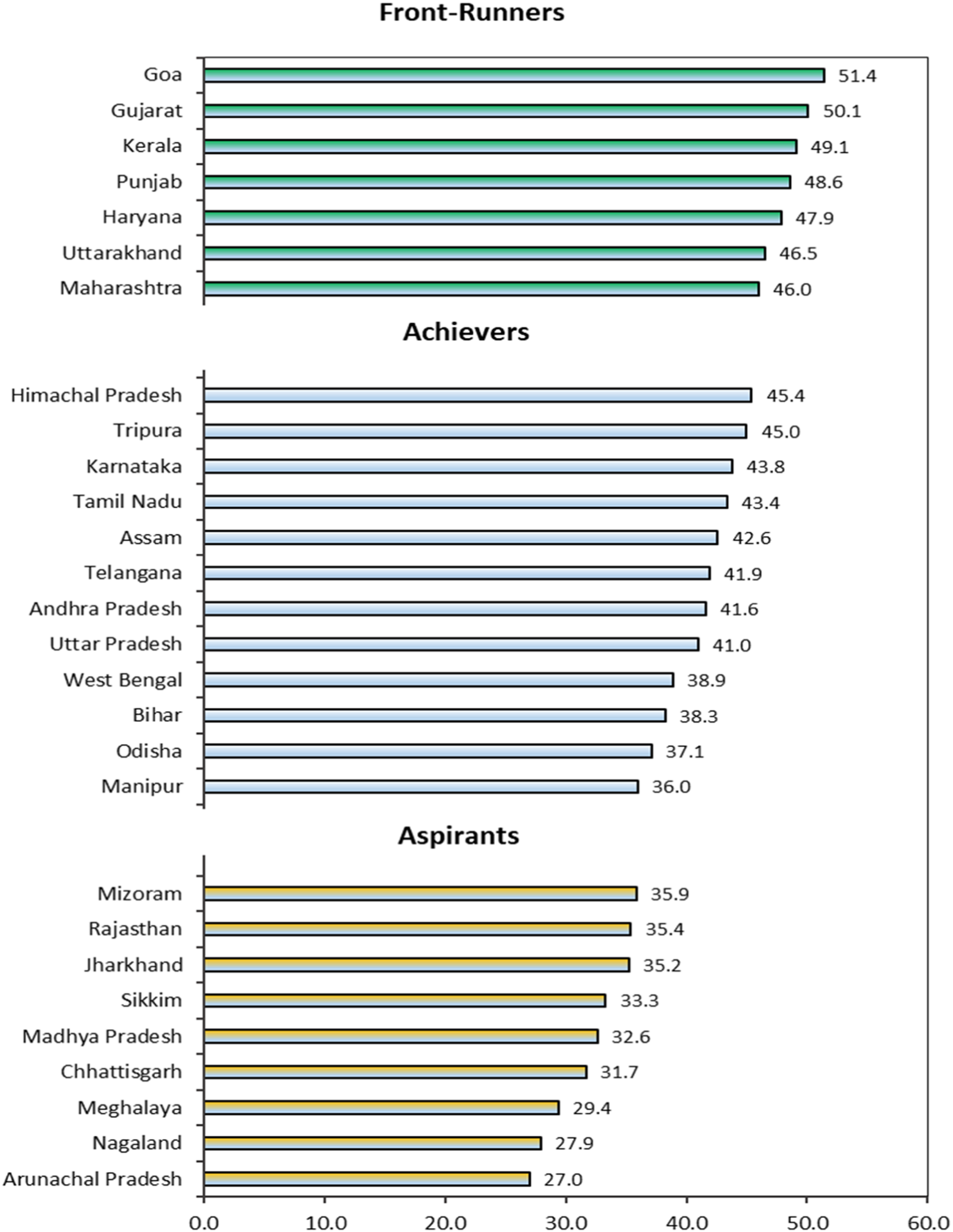

Derivation of weights and revised devolution formula

The empirical analysis confirms that income distance, geographic disadvantage, fiscal performance, demographic performance and, SECI have a significant impact on fiscal imbalance across states. Consistent with the FC’s objective of reducing vertical and horizontal fiscal imbalances, these five criteria should be incorporated into the formula. As discussed in the theoretical framework, not only should the selection of criteria be empirically justified, but their respective weights should also reflect their relative impact on fiscal imbalance.

However, as discussed in section 4.2, the coefficients obtained from the regression cannot be directly used as weights as they are non-comparable. To address this issue, the variables are transformed into standardized form and a standardized cross-section regression is estimated. The results of the standardized regression with comparable coefficients are presented in Table 3. The empirical strategy to derive weight for each significant criterion according to their relative importance is explained in section 4.2 (equation (10)).

Among the significant explanatory variables, income distance has the strongest influence on fiscal imbalance across states, followed by demographic performance and the GDI. The two performance-oriented indicators FPI and the SECI also show a meaningful and comparable effect on fiscal imbalance. As shown in Table 4, the highest weight is obtained for income distance (27%), followed by demographic performance (20%), GDI (19%), and 17% each for FPI and SECI. An advantage of deriving weights from empirical estimates is that the relative importance of equity and efficiency considerations in the devolution formula emerges from the data itself, rather than being determined through subjective judgement.

Table 4.

Criteria and weights under the revised formula.

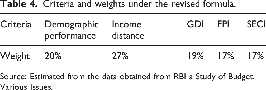
Criteria	Demographic performance	Income distance	GDI	FPI	SECI
Weight	20%	27%	19%	17%	17%

Source: Estimated from the data obtained from RBI a Study of Budget, Various Issues.

From the empirical analysis the share of each state is derived using the significant criteria and their respective weights. At first stage share of each state under individual criteria are calculated. After derivation of state’s share under individual criteria the share of each state in the total devolution pool is calculated by giving the derived weights on each criterion as shown in equation (11).

{S S D}_{i} = 0.27 {I D}_{i} + 0.20 {D P}_{i} + 0.19 {G D I}_{i} + 0.17 {F P I}_{i} + 0.17 {S E C I}_{i}

(11)

where SSD_i = total share of i^th state in total divisible pool.

ID_i = share of i^th state under income distance criterion.

DP_i = share of i^th state under demographic performance criterion.

GDI_i = share of i^th state under geographic disadvantage index criterion.

FPI_i = share of i^th state under fiscal performance index criterion.

SECI_i = share of i^th state under state energy and climate index criterion.

The total share of each state under the revised formula along with the corresponding change relative to the Fifteenth FC (FC) is reported in Table 5. Similar to earlier Commissions, the Fifteenth FC formula allocated the largest shares to states such as Bihar, Uttar Pradesh, West Bengal, and Madhya Pradesh. This allocation is partly justified since these states have larger populations and higher expenditure needs. However, the emphasis on population in the formula tends to inflate their shares disproportionately. The revised devolution formula, by contrast, incorporates fiscal capacity, expenditure needs, cost disadvantages, and efficiency considerations, and allocates shares based on empirical estimates. Under this framework, Uttar Pradesh receives the highest share (6.32%), followed by West Bengal (4.98%) and Bihar (4.82%), largely reflecting equity considerations. Most hilly states receive shares in the range of 3 to 4% due to their limited fiscal capacity and geographic disadvantages. The lowest shares are allocated to Goa, Haryana, and Punjab.

Table 5.

Share of each state under the revised formula (in percent).

States	15th FC	Revised formula	Change
Andhra Pradesh	4.04	3.57	−0.47
Arunachal	1.76	3.32	1.56
Assam	3.13	3.92	0.79
Bihar	10.07	4.82	−5.25
Chhattisgarh	3.41	3.59	0.18
Goa	0.39	2.27	1.88
Gujarat	3.48	3.51	0.03
Haryana	1.09	2.03	0.94
Himachal Pradesh	0.83	2.57	1.74
Jharkhand	3.31	3.70	0.39
Karnataka	3.65	3.55	−0.09
Kerala	1.92	2.97	1.05
Madhya Pradesh	7.86	4.49	−3.37
Maharashtra	6.31	4.71	−1.60
Manipur	0.72	3.60	2.89
Meghalaya	0.77	3.80	3.04
Mizoram	0.50	2.91	2.41
Nagaland	0.57	2.85	2.29
Odisha	4.53	4.06	−0.47
Punjab	1.81	2.28	0.48
Rajasthan	6.03	3.99	−2.04
Sikkim	0.39	2.73	2.34
Tamil Nadu	4.08	3.61	−0.47
Telangana	2.11	2.79	0.68
Tripura	0.71	4.23	3.53
Uttarakhand	1.12	2.80	1.68
Uttar Pradesh	17.95	6.32	−11.63
West Bengal	7.52	4.98	−2.55
Total	100	100	-

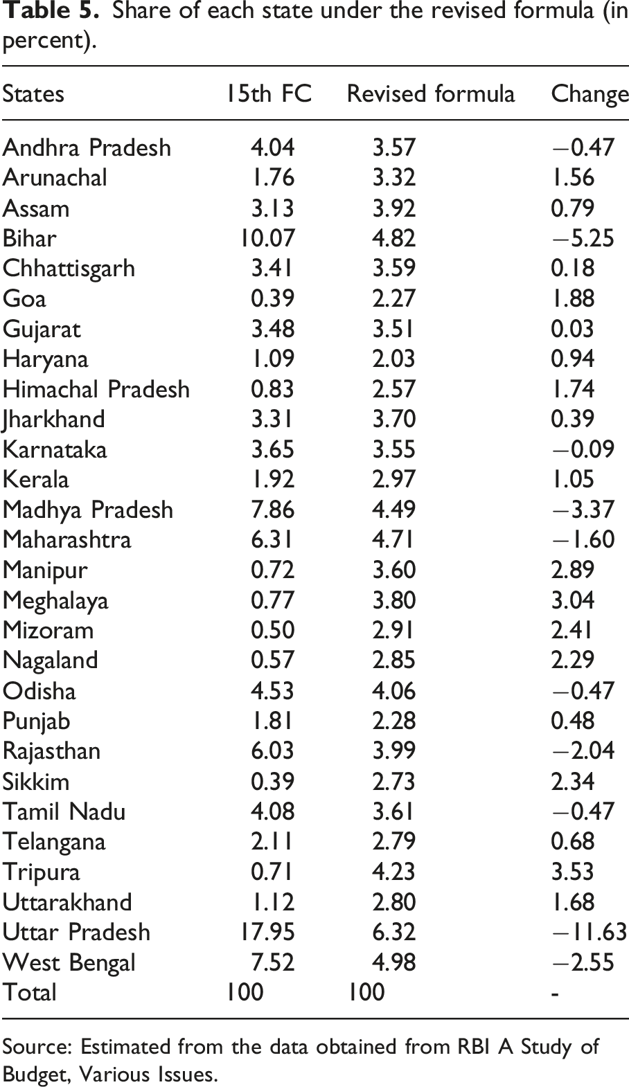
Source: Estimated from the data obtained from RBI A Study of Budget, Various Issues.

A comparative picture of the states under the Fifteenth FC devolution formula and the revised formula is illustrated in Figure 4. One limitation of both existing and previous devolution formulas has been the insufficient recognition of geographic constraints faced by certain states. As a result, the main differences between the two formulas arise from the inclusion of equity parameters such as income distance and the GDI. States that experience a reduction in share under the revised formula had previously benefited from the strong emphasis on population in the Fifteenth FC formula, where population influenced allocations both directly and indirectly. Conversely, states that gain under the proposed framework had received relatively smaller shares earlier due to lack of emphasis on geographic disadvantage as a criterion. States showing minimal change between the two formulas are generally those with stronger fiscal management, as reflected in higher values of the FPI.

Figure 4.

Comparative horizontal sharing. Source: Author’s illustration.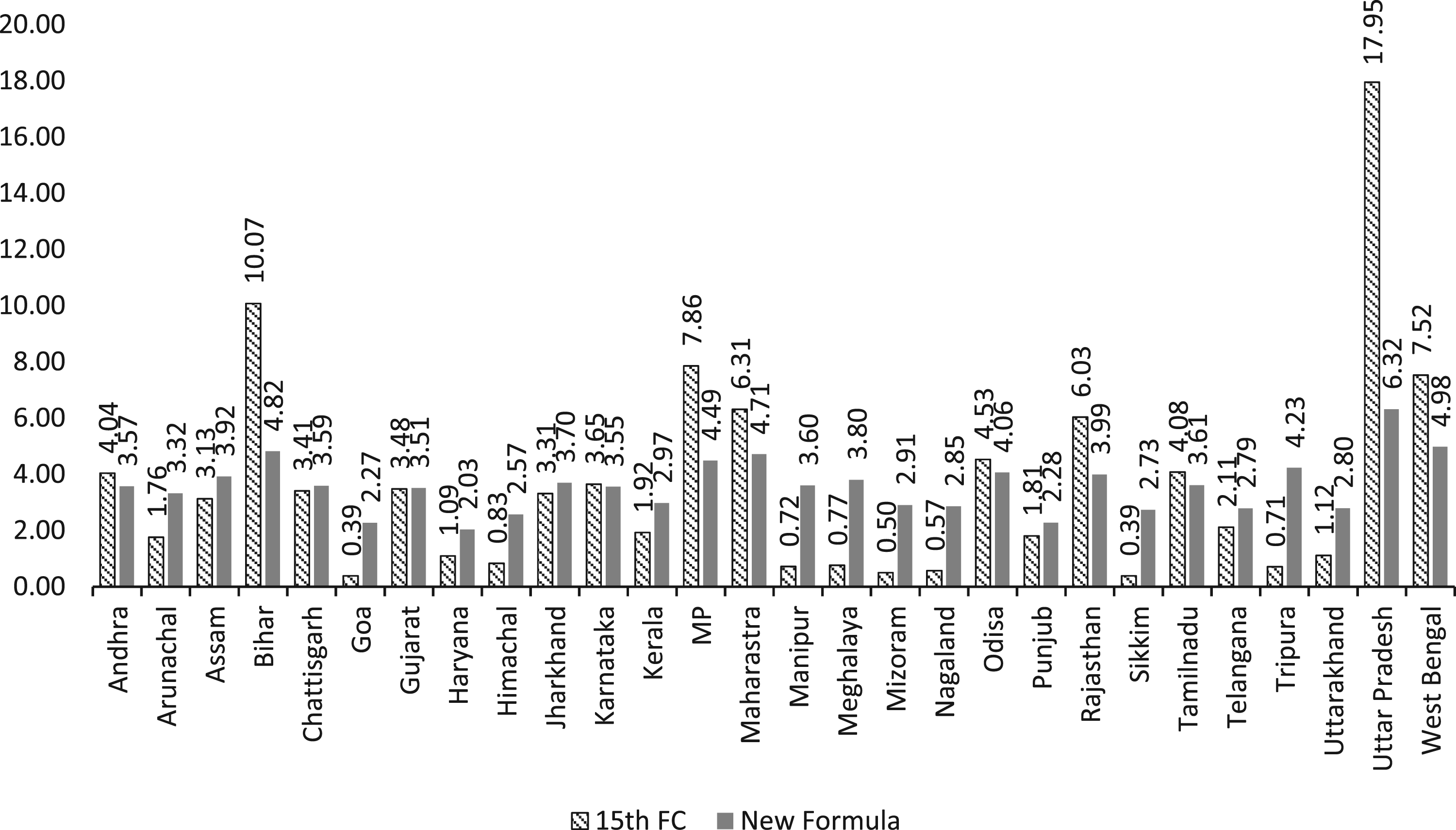

Under the revised formula, the major gainers are states characterized by hilly terrain and extensive forest cover, including Arunachal Pradesh, Himachal Pradesh, Mizoram, Meghalaya, Manipur, Nagaland, Tripura, and Sikkim. Among these, Tripura emerges as the largest gainer, primarily due to the recognition of its geographic disadvantages. In contrast, states such as Uttar Pradesh, Bihar, Madhya Pradesh, and West Bengal experience reductions in their shares, largely because the revised formula removes the superfluous use of population in final computation of each criterion, particularly income distance. The relative positions of the gaining and losing states are illustrated in Figure 5. Fiscally efficient states such as Gujarat, Karnataka, and Odisha show relatively little change under the revised formula. More comprehensible picture can be drawn from the share of the states under each criterion as reported in Table 6. Since demographic performance is derived from population weighted by reciprocal of total fertility rate, the states with higher population combined with low fertility rate are awarded the highest. Uttar Pradesh receives largest share (13.62%) for their high population. Maharashtra, on the other hand receives the second largest share of 10.48% attributed to low TFR or 1.91 combined with high population. The lowest shares are received by states with comparatively lower population such as Sikkim and Mizoram.

Figure 5.

Gainers and losers in the revised formula. Source: Author’s illustration.

Table 6.

Share of the states in criterion included in the revised formula.

States	Criteria (in percent)
States	Demographic performance	Income distance	GDI	FPI	SECI
Andhra Pradesh	5.60	3.10	1.92	3.64	3.70
Arunachal	0.11	3.62	7.76	2.57	2.40
Assam	2.57	6.02	2.52	3.85	3.79
Bihar	6.35	7.87	1.30	3.55	3.41
Chhattisgarh	1.88	5.27	2.65	4.74	2.82
Goa	0.17	0.87	1.50	5.53	4.58
Gujarat	5.31	1.82	1.99	4.83	4.46
Haryana	1.96	0.87	0.41	3.57	4.27
Himachal	0.70	1.17	4.60	3.25	4.04
Jharkhand	2.25	6.47	1.46	4.09	3.13
Karnataka	6.03	0.90	3.15	4.97	3.90
Kerala	3.36	0.87	4.13	3.18	4.37
MP	4.95	5.91	3.44	4.43	2.90
Maharashtra	10.48	1.29	3.94	4.84	4.10
Manipur	0.28	6.28	5.56	1.47	3.21
Meghalaya	0.15	5.97	6.18	3.19	2.62
Mizoram	0.08	2.56	6.15	2.88	3.20
Nagaland	0.17	4.52	5.44	0.85	2.48
Odisha	3.84	5.26	2.30	5.16	3.30
Punjab	2.69	2.91	0.82	0.42	4.33
Rajasthan	4.43	4.89	3.28	3.68	3.15
Sikkim	0.08	0.87	6.88	3.96	2.97
Tamil Nadu	8.15	1.28	1.71	3.84	3.86
Telangana	3.77	1.19	1.46	4.73	3.73
Tripura	0.38	4.90	9.09	2.50	4.01
Uttarakhand	0.85	1.22	5.63	3.07	4.14
Uttar Pradesh	13.62	6.79	2.38	4.05	3.65
West Bengal	9.82	5.33	2.36	3.16	3.46
	100	100	100	100	100

Source: Author’s Calculation.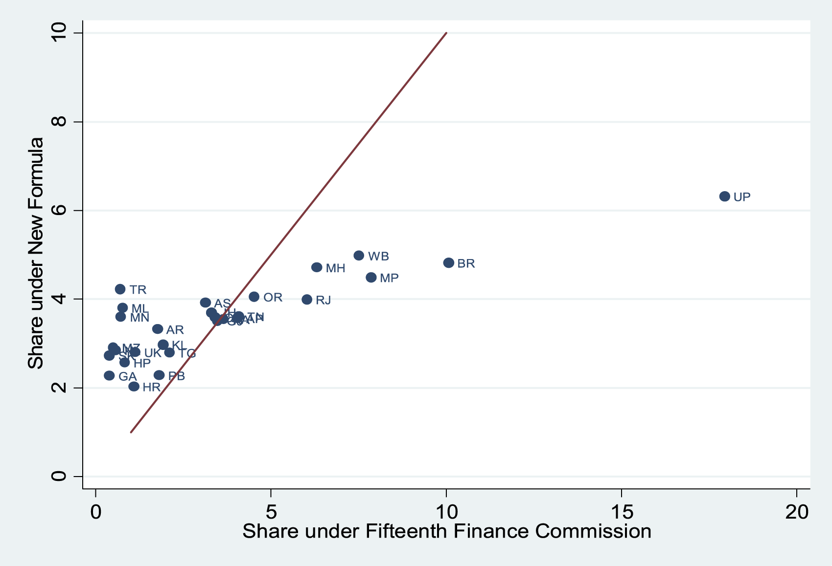

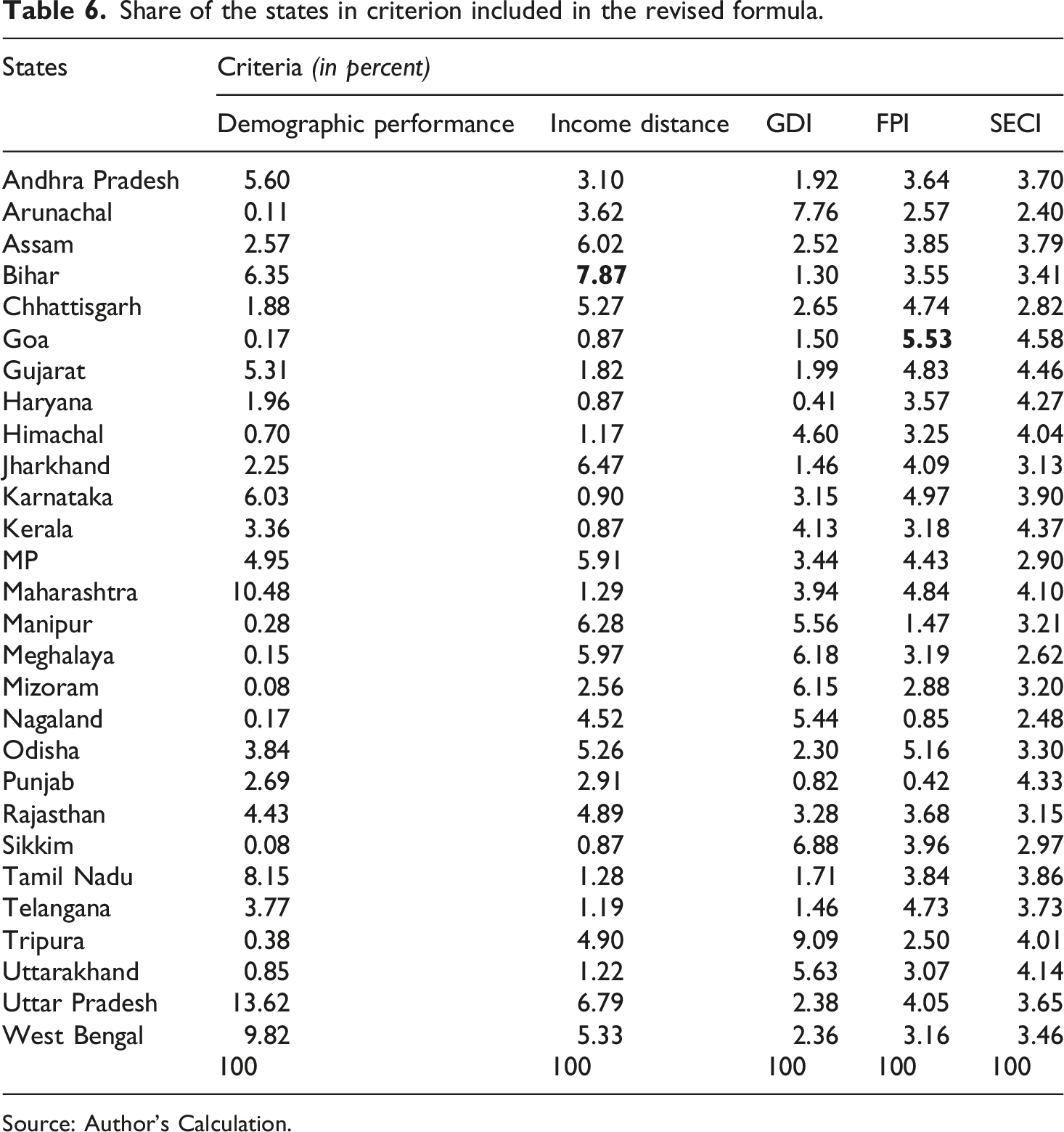
Income distance, the variable with highest implication for fiscal imbalance of a state represents the differences in fiscal capacity of the states. Bihar has the highest income distance from Haryana’s per capita income and entitled highest share 7.87% under income distance followed by Uttar Pradesh (6.79%). Under Fifteenth FC recommendations, Uttar Pradesh and Bihar were entitled spuriously larger share of 27.1% and 16.3%, respectively, attributed to their larger population. In contrast, hilly states, such as Arunachal Pradesh, Himachal Pradesh, and Nagaland that have low fiscal capacity indicated by distance of their per capita income from Haryana, received surprisingly smaller share of less than 1% as these states have comparatively lower population. After discarding the population bias from income distance, under revised formula the hilly states are entitled to their rightful share, purely based on their inadequate fiscal capacity (Table 6).

Under the Geographic Disadvantage Index (GDI), Tripura receives the highest share (9.09%), followed by Arunachal Pradesh (7.76%). Most hilly states receive relatively larger shares under this criterion due to their extensive forest cover and long international borders. In contrast, Haryana (0.41%) and Punjab (0.82%) receive the lowest shares under GDI.

Goa obtains the highest share under both the Fiscal Performance Index (FPI) and the State Energy and Climate Index (SECI), reflecting its top ranking in these efficiency-based indicators. Odisha, which demonstrates strong fiscal prudence across deficit management, debt sustainability, revenue effort, expenditure quality, and self-sufficiency, receives a share of 5.16% under the FPI criterion. At the other end, Punjab records the lowest fiscal performance due to weak expenditure quality and high fiscal and revenue deficits, receiving only 0.42% under FPI. Assam shows a moderate level of fiscal performance and receives a share of 3.85% under this criterion. Other NE states such as Arunachal Pradesh, Nagaland, Manipur, and Mizoram receive relatively lower shares under FPI, largely due to their high dependence on fiscal transfers and relatively weak revenue effort.

After Goa, Gujarat is entitled second highest share of 4.46% due to efficiency in energy usage and climate change management. Gujarat is the front runner in state energy and climate index among the large states. Lowest share in SECI is obtained by Arunachal Pradesh (2.40%) as compared to other states the performance of energy DISCOM’s are inefficient combined with low energy efficiency. The progressivity³ of each criterion is depicted in Table 7. Clearly, income distance is progressive as showed by the significant negative correlation coefficient. State energy and climate index is regressive as the poorer states are lagged in case of efficiency in energy transition and environmental sustainability.

Table 7.

Progressivity of each criterion (correlation with GSDP per capita).

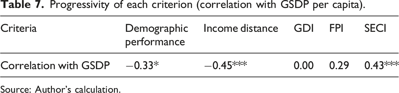
Criteria	Demographic performance	Income distance	GDI	FPI	SECI
Correlation with GSDP	−0.33*	−0.45***	0.00	0.29	0.43***

Source: Author’s calculation.

Conclusion

The present study proposes an empirically grounded framework in which both the criteria and their weights are derived from their observed impact on fiscal imbalance. Based on the theoretical framework, six indicators, demographic performance, income distance, FPI, GDI, SECI, and population index, are included in the empirical analysis. Among these, SECI, FPI, GDI, demographic performance, and income distance significantly affect fiscal imbalance and therefore merit inclusion in the formula-based proposed devolution framework. Based on their relative importance we derived weights for each significant criterion with income distance (27%) obtaining the highest weight followed by demographic performance (20%), GDI (19%), SECI (17%), and FPI (17%). Comparison with the Fifteenth FC’s devolution scheme shows that some states were placed in highly advantageous positions, while states facing geographical disadvantages received relatively lower shares.

Major losers under the revised formula include Bihar, Madhya Pradesh, Maharashtra, Uttar Pradesh, Rajasthan, and West Bengal. Notably, Uttar Pradesh, Bihar, and West Bengal continue to retain the highest shares, as in the Fifteenth FC’s recommendations. The reduction in their shares arises mainly from the removal of the overwhelming emphasis on population. This change results from modifying the income distance criterion, where the additional population weighting previously embedded in the measure has been removed in the revised formula.

Major gainers under the revised methodology include the NE states and hilly states such as Himachal Pradesh and Uttarakhand. This improvement reflects the inclusion of the GDI, which captures the challenges faced by states with difficult terrain and geographical constraints. The revised formulation thus provides greater recognition of state-specific characteristics while aligning with the objectives of equalizing fiscal capacity, addressing expenditure needs, accounting for differences in the cost of providing public services, and incentivizing efficiency in demographic, environmental, and fiscal performance.

Although the empirical analysis focuses on Indian states, the methodological approach has broader relevance for other fiscal federal systems. Many federations-including Canada, Australia, and Germany face similar challenges in designing devolution formulas that balance equity, efficiency, and incentive compatibility. The empirical framework developed here, which derives both criteria and weights from their statistical relationship with fiscal imbalance, can be adapted to other federal systems where intergovernmental transfers aim to equalize fiscal capacity while accounting for regional heterogeneity. The criteria or indicators can vary across regions and can be customized according to individual specifications. The principle of linking transfer design to empirically observe determinants of fiscal imbalance remains widely applicable.

The existing empirical literature and the framework adopted in successive Finance Commission devolution formulas focus on the static nature of fiscal imbalance, highlighting the revenue side. The present study also addresses the problem of fiscal imbalance considering similar aspect, while partially adding the expenditure side by incorporating indicators related to geographic constraints that inflate cost of providing public goods. However, the dynamic dimensions of fiscal federalism can be incorporated in further studies which is linked to long-term growth performance of the states. Inclusive growth, emphasized in the Sustainable Development Goals (SDGs), depends significantly on investments in both physical and human capital through public capital formation. Therefore, as noted by Raychaudhuri and Roy⁵¹ the focus should be on public capital which is the primary driver of inclusive growth and ensures the long-term effectiveness of fiscal equalization in promoting balanced regional development. Future research may therefore incorporate indicators related to public investment and growth performance to better capture the dynamic dimensions of fiscal federalism.

Supplemental material

Supplemental material - Finance commission transfers in India: An alternative approach to the devolution process

Supplemental material for Finance Commission transfers in India: An alternative approach to the devolution process by Nitu Moni Bora, Nissar A. Barua in Journal of Economic and Social Measurement

Footnotes

ORCID iD

Nitu Moni Bora

Funding

The authors disclosed receipt of the following financial support for the research, authorship, and/or publication of this article: The corresponding author received funding in the form of fellowship (Junior Research Fellow) by University Grants Commission (UGC) during the study.

Declaration of conflicting interests

The authors declared no potential conflicts of interest with respect to the research, authorship, and/or publication of this article.

Supplemental material

Supplemental material for this article is available online.

Notes

References

Sarma

JVM

. Federal fiscal relations in India: issue of horizontal transfers federal fiscal relations in India issue of horizontal transfers. Econ Polit Wkly 1997; 32: 1719–1723.

Bagchi

. Fifty years of fiscal federalism in India. Artha Vijnana 2002; 44: 1–46. https://doi.org/10.21648/arthavij/2002/v44/i1/115829

Sarma

JVM

. Federal fiscal relations in India: imperatives for restructuring. Sage India, 2020.

Bhaskar

Subrahmanyam

. Population as a criterion for horizontal devolution by the 14th finance commission. Econ Polit Wkly 2014; 49: 20–23.

Das

Mishra

. Horizontal equity and the thirteenth Finance commission: issues and ponderables. Gujarat Institute of Development, 2008.

Sahu

Mahamallik

Mahapatra

. Recommendations of the 15th Union Finance Commission: expectations and realities. Indian Econ J 2024; 72: 159–167. https://doi.org/10.1177/00194662231203460

Chakraborty

Gupta

. Terms of reference of the Fifteenth Finance Commission: use of 2011 population and horizontal inequality. In: The Routledge Handbook of Post-Reform Indian Economy. Routledge India, 2021, pp. 239–258.

Subrahmanyam

. Finance commission transfers in India: a critical note. Indian Econ Rev 1988; 23: 121–138.

Guhan

. Devolution Criteria: From Gamble to Policy. Econ Polit Wkly 1984; 19: 2036–2044.

10.

Vidwans

. Finance commissions: perilous proxies and dangerous dummies. Econ Polit Wkly 1999; 34: 2725–2734.

11.

Chelliah

. Review Article : Report of the Finance Commission 1978. 1979; 14: 51–64.

12.

Kumar

. Regional development criteria and horizontal devolution under the finance commission awards. Econ Polit Wkly 2001; 36: 4671–4675.

13.

Bajaj

Viswanathan

. Financial management in states: role of finance commission. Econ Polit Wkly 1989; 24: 2255–2266.

14.

Godbole

. Finance commissions in a cul-de-sac. Econ Polit Wkly 2001; 36: 29–34.

15.

Arun

. Poverty ratio as A devolution criterion: a note. Econ Polit Wkly 1989; 24: 319–321.

16.

Sethia

. Fiscal federalism and redistributive politics in India. Working Paper No WP/06/016/ECO, Indian Institute of Management, Indore.

17.

Bagchi

Datta

Choudhury

. Poverty measures as an index of backwardness and their relevance for tax devolution poverty measures as an index of backwardness and their relevance for tax devolution. Econ Polit Wkly 1989; 24: 831–836.

18.

Sarmah

Panda

. Intergovernmental transfers and fiscal equalization across the north-eastern states of India: evidence from panel data. J Public Aff 2023; 23: e2872. https://doi.org/10.1002/pa.2872

19.

Busch

Mukherjee

. Encouraging state governments to protect and restore forests using ecological fiscal transfers: india’s tax revenue distribution reform. Conserv Lett 2018; 11: 1–10. https://doi.org/10.1111/conl.12416

20.

Xavier

FAD

Mukhopadhyay

. Can fiscal transfers help India meet its SDG goals? South Asian Journal of Macroeconomics and Public Finance 2023; 12: 218–249. https://doi.org/10.1177/22779787231168771

21.

Sahu

Mahamallik

Mahapatra

. Recommendations of the 15th Union Finance Commission: expectations and realities. Indian Econ J 2024; 72: 159–167. https://doi.org/10.1177/00194662231203460

22.

Srivastava

. Resolving vertical and fiscal imbalances in India: a task for the Sixteenth finance commission. Indian Econ J 2025; 73: 132–152. https://doi.org/10.1177/00194662241303987

23.

Shah

. A practitioner’s guide to intergovernmental fiscal transfers. In: Boadway

Shah

(eds). Intergovernmental Fiscal Transfers: Principal and Practice. World Bank, 2007, pp. 1–51.

24.

Boadway

Shah

. Fiscal federalism: principles and Practice of multiorder Governance. Cambridge University Press, 2009.

25.

Dougherty

Nebreda

Mota

. Adapting intergovernmental fiscal transfers for the future: emerging trends and innovative approaches. In: OECD Working Papers on Fiscal Federalism, vol 49. https://doi.org/10.1787/6389ca23-en

26.

Brenton

. The price of Federation: comparing fiscal equalization in Australia, Canada, Germany and Switzerland. Reg Fed Stud 2020; 30: 93–111. https://doi.org/10.1080/13597566.2019.1658082

27.

Bagchi

. Readings in public finance, 2005. https://philpapers.org/rec/BAGRIP (accessed 7 March 2026).

28.

Rangarajan

Srivastava

. Federalism and fiscal transfers in India. Oxford University Press, 2024.

29.

Bhutani

Mishra

. India’s perverse fiscal federalism: some suggestions for the 15th Finance Commission. J Public Aff 2022; 22: e2523. https://doi.org/10.1002/pa.2523

30.

Pattnaik

. Indian fiscal federalism: a study of factors affecting resource position of the state governments. J Soc Econ Dev 2019; 21: 191–211. https://doi.org/10.1007/s40847-019-00087-9

31.

Reddy

. Indian fiscal federalism. Oxford University Press, 2018.

32.

Mukhopadhyay

Das

. Horizontal imbalances in India issues and determinants. Econ Polit Wkly 2003; 38: 1416–1420.

33.

Sen

Trebesch

. Use of socio-economic criteria for intergovernmental transfers. Econ Polit Wkly 2004; 39: 2748–2755.

34.

Tiebout

. A pure theory of local expenditure. J Polit Econ 1956; 64: 416–424. https://doi.org/10.1086/257839

35.

Dholakia

. Measuring fiscal performance of states: an alternative approach. Econ Polit Wkly 2005: 3421–3428.

36.

Bora

Barua

. Management of fiscal imbalance through intergovernmental transfers in India: an empirical study. Indian J Econ 2020; 101: 331–349.

37.

NITI Aayog . State energy and climate index: round I. https://www.niti.gov.in/sites/default/files/2021-08/State-Energy-Climate-Index-Round-I_0.pdf 2021.

38.

Wooldridge

. Econometric analysis of cross section and panel data. MIT Press, 2002.

39.

Baltagi

. Limited dependent variables and discrete choice modelling. Oxford Research Encyclopedia of Economics and Finance, 2021.

40.

Neter

Wasserman

Kutner

. Applied linear statistical models. Richard D. Irwin. Inc, vol 842.

41.

Wooldridge

. Introductory econometrics a modern approach. South-Western cengage learning, 2016.

42.

Bring

. How to standardize regression coefficients. Am Stat 1994; 48: 209–213. https://doi.org/10.1080/00031305.1994.10476059

43.

Nardo

Saisana

Saltelli

, et al. Handbook on constructing composite indicators: methodology and user guide. OECD Publishing, 2008. https://www.oecd.org/sdd/42495745.pdf

44.

Loh

W-Y

Zhou

. Variable importance scores. J Data Sci 2021; 19: 569–592. https://doi.org/10.6339/21-jds1023

45.

OECD . Handbook on constructing composite indicators: methodology and user guide. Organisation for Economic Co-operation and Development, 2008. https://www.oecd.org/sdd/42495745.pdf

46.

Nieminen

. Application of standardized regression coefficient in meta-analysis. BioMedInformatics 2022; 2: 434–458. https://doi.org/10.3390/biomedinformatics2030028

47.

Kharas

Rivard

. Debt, creditworthiness, and climate A new development dillema. Center for Sustainable Development, Brookings.

48.

Bloom

Sousa-Poza

. Economic consequences of low fertility in Europe. Eur J Popul 2010; 26: 127–139. https://doi.org/10.1007/s10680-010-9209-7

49.

Golley

Tyers

. Contrasting giants: demographic change and economic performance in China and India. Procedia Soc Behav Sci 2013; 77: 353–383. https://doi.org/10.1016/j.sbspro.2013.03.093

50.

Azam

Bhatt

. Spatial income inequality in India, 1993-2011: a district level decomposition. IZA Discussion Papers, No 9892, Institute for the Study of Labor (IZA), Bonn.

51.

Raychaudhuri

Roy

. The optimal distribution rule of federal funds to states in India: a suggested methodology. South Asian Journal of Macroeconomics and Public Finance 2021; 10: 193–225. https://doi.org/10.1177/2277978721989921

Supplementary Material

Please find the following supplemental material available below.

For Open Access articles published under a Creative Commons License, all supplemental material carries the same license as the article it is associated with.

For non-Open Access articles published, all supplemental material carries a non-exclusive license, and permission requests for re-use of supplemental material or any part of supplemental material shall be sent directly to the copyright owner as specified in the copyright notice associated with the article.

0.68 MB

0.00 MB