
Abstract
This conceptual and practical overview of multilevel modeling (MLM) for researchers in counseling and development provides guidelines on setting up SPSS to perform MLM and an example of how to present the findings. It also provides a discussion on how counseling and developmental researchers can use MLM to address their own research questions.
The potential usefulness of quantitative methods for counseling researchers was highlighted in a recent special section of the Journal of Counseling and Development (Balkin & Sheperis, 2011; Hunt & Trusty, 2011; Trusty, 2011). Graduate training programs in counseling and counselor education generally strive to find a balance between quantitative and qualitative methods in the course work required of their students and can at best expose counselors-in-training to a selection of the most essential quantitative techniques. As a result, counseling researchers who wish to conduct a quantitative study are sometimes restricted in the kind of question they are able to investigate by the statistical tools they have at hand. In addition, they may feel intimidated to explore some of the newer techniques that are available but that are rarely covered in graduate training programs.
One of those newer techniques that may be of particular interest to counseling and developmental researchers is multilevel modeling (MLM). MLM provides a way to analyze data that are hierarchically structured, such as when individuals are embedded within some other unit, such as hospitals, clinics, or schools. Indeed, MLM has been fairly widely used in the field of education (e.g., Bock, 1989; Raudenbush, 1988), and although efforts have been made to introduce the approach to researchers in personality psychology (e.g., Fleeson, 2007) and counseling psychology (e.g., Kahn, 2011; Reise & Duan, 1999), it remains unfamiliar to many students, educators, and practitioners in the fields of professional counseling and human development. The present overview is written with this audience in mind. First, I provide a conceptual overview of MLM using Bronfenbrenner’s ecological systems schema as a framework. Second, existing reviews typically present MLM in a way that relies on the use of equations, esoteric terminology, Greek letters, and unfamiliar statistical software packages and do not discuss the mechanics of how to perform the actual MLM analysis. As a result, MLM remains potentially intimidating to the nonstatistician or to the researcher who, for reasons of economy of finances or time, cannot afford to learn a new technique or how to use a new statistical software package. In contrast, the present overview minimizes the use of statistical jargon and describes, step by step, how a statistical software program with which many readers are already likely to be familiar, IBM SPSS Statistics (SPSS; Norusis, 2011), can be made to conduct an analysis of a basic multilevel model. Following this step-by-step walkthrough is a discussion of how to interpret the output provided by SPSS. A sample data set from my own research is made available for readers to follow along and test their understanding of the procedure. Finally, based on this data set an example is provided to show how the Methods and Results sections might be written for a study that makes use of MLM. Thus, this article will serve as a brief, conceptual, and practical guide to MLM for researchers in counseling and development.
Conceptual Overview of Multilevel Modeling
As its name implies, multilevel modeling (MLM) involves testing the influence of variables that exist at different levels of analysis. To clarify what this means, researchers in counseling and human development might find it helpful to think in terms of Bronfenbrenner’s ecological model (Bronfenbrenner, 1979, 2004). According to Bronfenbrenner, human development involves continuity and change as both proximal and distal systems in the environment influence and interact with the individual. Human beings are typically embedded within families, which in turn are embedded within neighborhoods and communities, which themselves are in turn embedded within larger social and cultural systems. (In the language of MLM, we might say that persons are nested within families, families are nested within communities, and so on.) Each successive level of the environment exerts its influence on the person either directly or indirectly, through other, typically more proximal, levels. Traditionally, researchers interested in studying environmental or contextual effects have been limited to studying one level of influence on the person while being forced by their data analytic strategy to ignore other, possibly equally important, levels of the environment. In addition, traditional methods such as regression analysis typically adopt a one-size-fits-all approach, in which any association among variables is assumed to be the same for everyone in the sample. Among other things, MLM allows researchers to test research questions that involve multiple levels of influence and to test whether associations between variables might be different for different people in the sample.
The ecological metaphor is an important one because counselors often think in terms of a systems approach and in terms of contextual influences on the person. The notion of levels of analysis needs to be unpacked a bit further, however, to truly appreciate the exciting potential of MLM. In this regard, it is especially important to understand the concept of nesting, how between-persons factors are different from within-persons factors, and how, based on these concepts, MLM allows researchers to move beyond the study of structure to the study of process, a distinction that will be discussed more fully below.
As mentioned earlier, nesting of data happens when one unit of observation is embedded within another unit of observation. Based on this principle, there are two primary configurations of data that typically are of interest to developmental and counseling researchers, each of which will be described in turn: when people are nested within some larger ecological setting and when variables are nested within the person. A study in a school environment might serve as an example of the first type of nesting. In such a study, we might collect data from students in just one classroom, but it might also be possible to collect data from students in multiple classrooms. In this case, students would be nested within classrooms (or within teachers, depending on the focus of one’s study). Importantly, MLM does not require that this second level of analysis, classroom, be treated as a “dummy” variable, as in regression analysis; rather, aspects of the classroom can also be measured and included in the study. This is helpful, because it provides a way to test whether variations in a particular student variable or variables are associated with variations that take place at the level of classrooms (or teachers). For example, are variations in teaching style associated with variations in student motivation? It might be possible to extend the study even further and collect data from students in classrooms across multiple schools in the school district, in which case students would be nested in classrooms, and classrooms would in turn be nested within schools. If we then included several different school districts in the study, schools would be nested within districts. Analogously, we might study all the clients being seen by all the counselors in a particular school or agency, and then include multiple schools or agencies; clients would be nested within counselors, counselors nested within agencies, and so on. In reality, most studies do not look beyond two or three levels of analysis, for practical reasons (e.g., involving the cost of data collection) and for statistical reasons involving issues of power (see Balkin & Sheperis, 2001; Reise & Duan, 1999), and because, as Bronfenbrenner’s model suggests, we typically think in terms of the more proximal levels of the ecological system having the more immediate impact on the person. But from this we can see conceptually how nesting refers to data that are hierarchically organized.
In the examples above, the nesting of data in a hierarchical arrangement was described in terms of Bronfenbrenner’s ecological model, with individual persons being nested within ever wider environmental contexts. As previously mentioned, variables can also be nested within individuals. Indeed, an interesting feature of MLM is that it can be applied to the study of things happening within the individual, providing a window into within-person processes. Process is typically contrasted with structure. As Fleeson (2007) noted, process “refers to a combination of actions, changes, or events that bring about an outcome,” with the implication that processes may be unique to each person, whereas structure “consists of variables . . . and their typical or fixed relationships to each other” (pp. 523, 524). The potential of a within-person approach for the study of process will become apparent by contrasting it with the more traditional between-persons approach.
Between-persons approaches capture differences between individuals. For many years, this was the standard approach used in empirical studies in psychology, which tended to focus on individual differences. The focus of such research was necessarily on structure, that is, on the stable characteristics of personality rather than on process, or the dynamic interplay of forces in the person and in the environment that bring about change. This was as much due to methodological limitations as to philosophical commitment. A researcher using a between-persons approach typically tests whether differences between people in an explanatory variable are associated with differences between people on some outcome variable: For example, do people who experience a greater number of stressors in their life tend to score higher on a measure of depression? The results of a between-persons analysis show whether there are associations between two variables at the group level, on average. If there is an association between two variables, an assumption is often made that the strength and direction of the association is basically the same for all individuals in the group, and that, by adjusting the level of the explanatory variable in a given person, the level of the outcome for that person should change, accordingly. Descriptive findings at the level of the group are often transformed into prescriptive interventions at the level of the individual, something that has been referred to as the ecological fallacy (Fleeson, 2007; Robinson, 1950). This type of analysis is traditionally performed with the use of regression.
In contrast, within-person approaches capture differences across multiple observations that are made within each individual unit. Here, the unit is the person. (When the study involves people nested within some larger context, as in the examples given earlier, multiple observations are also recorded within each individual unit, but in those cases the unit is a classroom with multiple students, or a counselor with multiple clients.) In the language of empirical research, an observation is any piece of data that has been recorded. When the data collection takes place over time, longitudinally, observations may be thought of as occasions, and indeed MLM provides a useful way to study variations across occasions (i.e., over time), as those variations are observed within individual people. MLM, in other words, provides a way of studying change. Experience sampling, in which individuals report their behavior, attitudes, or emotions multiple times during the day over the course of a week or several weeks, usually with the help of a handheld computer or other device, is an example of a methodology that provides within-person data, recorded over time, that can be analyzed using MLM (see Fleeson, 2001, for an example).
But MLM is not limited to looking at variations over time. MLM can also address questions that involve looking at within-person variations that occur across observations, more generally speaking. For example, a researcher might be interested in studying how a person’s behavior varies from one situation, context, or relationship to another. Lynch, La Guardia, and Ryan (2009), for example, asked participants to respond to items tapping how they thought about themselves (their self-concept) when with a number of relationship partners, and compared this with the participants’ self-endorsed ideal self-concept. They also measured the degree of autonomy support participants experienced when with each of those partners. Using MLM, the researchers found a reliable, within-person association linking variations in self-concept with variations in perceived autonomy support. For the typical person in the study, being with an autonomy supportive partner was associated with being closer to one’s own ideal self-concept.
In general, when data for each individual participant are collected either as multiple observations over time or as multiple observations across situations, those observations are said to be nested within individuals. When observations are nested within individuals, they potentially lend themselves to an MLM approach that tests for the presence of a within-person process. This stems from the characteristic of MLM noted earlier, that both explanatory and outcome variable, far from being static, can fluctuate from observation to observation, making it possible to talk about within-person processes in a more meaningful way. This point is important to note, because it calls attention to the fact that MLM is not only appropriate for handling data that are hierarchically nested in the ecological systems sense but is also suited to addressing questions that focus on process rather than simply on structure, that is, on within-person variations reflecting the dynamic interplay of person and environment rather than static individual differences (e.g., personality traits that are believed to be stable) observed at the group level. The ability to test within-person variations over time, and to test within-person variations across interpersonal contexts, may be of special interest to counseling and developmental researchers, something that will be addressed more fully in the Discussion section.
Perhaps the most unique feature of MLM is that it allows for the possibility that the strength, the direction, or even the presence of an association between the explanatory variable and the outcome may be different for different people. In the study noted above (Lynch et al., 2009), researchers found that although for the typical person in the sample there was a positive association between autonomy support and ideal self-concept in one’s relationships, the association was not the same for everyone: For some it was stronger, for others weaker, and for some it may not have been present at all. To anticipate, MLM provides two types of coefficient to convey this information: a coefficient similar to the beta in a regression analysis, which indicates the presence, strength, and direction of an association between the explanatory and outcome variables for the typical individual, and a coefficient that indicates whether or not that association is the same for each person in the sample. The latter coefficient is essentially a standard deviation on the beta, and SPSS provides a test of its significance, as well. If this second coefficient is statistically significant, it suggests that the association between explanatory and outcome variables is different for different people. It is important to point out how radically different this is from traditional regression analysis: whereas regression assumes the association between variables is the same for all people in the sample (even though people may start off at different levels on one or both variables), MLM makes no such assumption. With MLM, researchers can test what they intuitively recognize: that within-person processes relating one variable to another may be different for different people (see Kalaian, 2003, for a similar argument).
Reise and Duan (1999) called attention to two statistical advantages that MLM has over other approaches. First, data that are nested generally are not statistically independent: For example, clients who see the same counselor are likely to have similarities to each other that are not random. Failing to take this kind of “nonindependence” into account can invalidate the results of one’s analysis. This problem is bypassed by MLM, however, because it expressly takes the statistical dependence of nested data into account. The second issue is that most types of analysis require a “balanced design,” that is, they require that the number of members in each group be the same. This is not the case with MLM, which allows there to be a different number of participants or observations for each group. Thus, in addition to the conceptual issues that may make MLM attractive to researchers, there are important statistical considerations, as well.
Using SPSS to Test a Multilevel Model
This section highlights some of the key issues and the basic steps in conducting an MLM analysis, illustrated at various points with a selection of data from a real data set, to be described below. The presentation is necessarily simplified, but should provide enough guidance to test a basic MLM model. The interested reader is directed to other sources for more detailed discussions (e.g., Bryk & Raudenbush, 1987; Fleeson, 2007).
As a point of reference, this presentation will use data from a study of mine that is reported in full elsewhere (Lynch, 2012). Accordingly, detailed information on the context of the study, the measures used, and so on, is omitted here; interested readers are referred to the original study. In brief, the study looked at how attachment security (here represented by attachment avoidance) and autonomy support contribute to a motivational construct called emotional reliance, which is the willingness to seek interpersonal support during an emotionally salient event (see Ryan, La Guardia, Solky-Butzel, Chirkov, & Kim, 2005). This example study makes use of data that are nested within individual persons.
In most published research, MLM has typically been conducted using a program called HLM, which stands for hierarchical linear modeling (Bryk, Raudenbush, & Congdon, 1996). HLM is a powerful program that has set the standard for conducting MLM analyses. One drawback, however, is that for new users it provides a few hurdles to overcome, including the need to learn a new program and the need to work with symbols and equations that may be unfamiliar. Thankfully, Fleeson (2007), writing primarily with personality psychologists in mind, has provided a step-by-step guide for how to conduct a basic MLM analysis using SPSS. I have adapted his instructions and clarified them at certain points where it seemed to me further elaboration was required. Readers will find this section easier to follow if they have SPSS open on their computer.
The first issue in getting SPSS to perform an MLM analysis has to do with how the data are structured. When data are entered into an SPSS spreadsheet, there is usually only one row of data for each participant. Variables are generally set up as columns across the spreadsheet, with each column representing a different variable. Recall, however, that in MLM, at least some of the variables have been recorded multiple times for each participant—either as multiple observations across occasions (i.e., over time), or as multiple observations across situations (e.g., across different relationships). These within-person variables, called Level 1or random variables in the language of MLM, need to be set up not as columns, but as rows, in SPSS. (Level 2 variables are those that are fixed, i.e., those that do not change from observation to observation, e.g., a personality trait or some other individual difference measure.) Setting up variables as rows can be done using the “Restructure” command in SPSS. (Note that it is always a good idea to save a backup copy of the original data file, before restructuring.) To restructure a data set to prepare it for an MLM analysis, first be sure that there is a variable called “ID” in which is recorded a unique identifier for each participant. Often this is the first column on the spreadsheet. Then open the drop-down Data menu in SPSS, and select “Restructure.” On the screen that appears, select “Restructure selected variables into cases.” After following the onscreen instructions, the data should now be set up in such a way that each individual participant is represented by multiple rows. Figure 1 shows an example of data in a spreadsheet before and after restructuring. In the top panel, data for the variable, autonomy support (“AS”), are recorded as columns across four relationships for each participant; after restructuring, however, each participant is represented by four rows, one row for each relationship (1 = mom, 2 = dad, 3 = best friend, 4 = romantic partner). Inspecting the data after restructuring should show that each row corresponds to an occasion or observation and that these occasions are sorted by participant ID, providing a visual confirmation of the within-persons nature of the data.
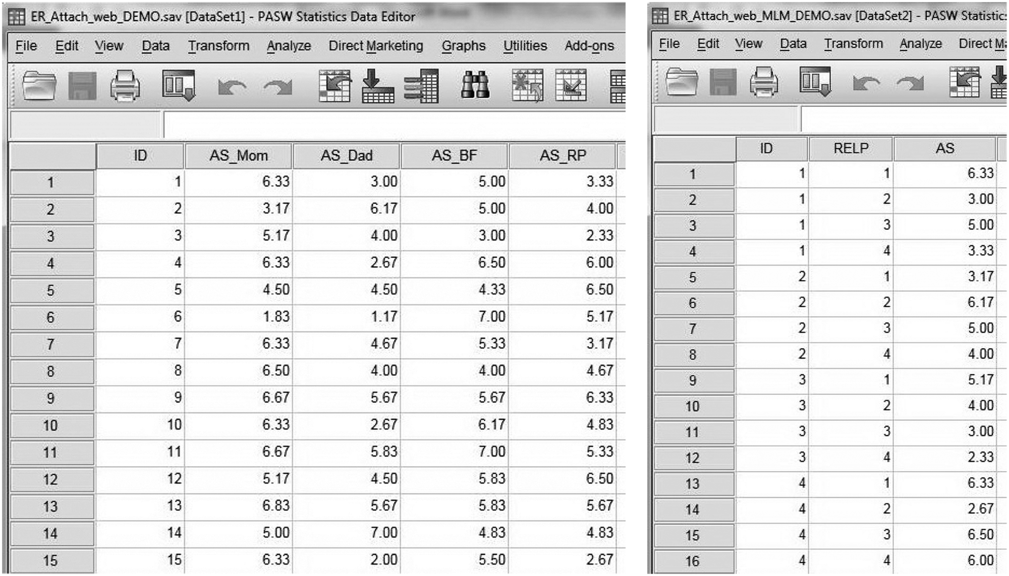
Data set before and after restructuring: Autonomy support (AS) as four columns per participant becomes four rows per participant
A second consideration has to do with centering the explanatory variables. (Note that only explanatory variables, sometimes called independent or predictor variables, are centered.) Most texts recommend mean-centering all explanatory variables on the group mean before performing a traditional between-persons regression analysis (e.g., Aiken & West, 1991; Meyers, Gamst, & Guarino, 2006). There are a number of reasons for this, one of which is to reduce the chances of multicollinearity among the explanatory variables. As Fleeson (2007) points out, centering is also important in MLM analyses, but because MLM uses within-person data the centering of any Level 1 variable must be done within persons. The main reason is that centering within persons helps ensure that results reflect a pure description of within-person processes and are not contaminated by any between-persons variance. For example, if one is measuring perceived autonomy support across a set of partners, centering on one’s own mean accounts for the possibility that some people are characteristically more likely to perceive their partners as autonomy supportive. Centering within persons in an MLM analysis involves using the “Aggregate” command in SPSS. Note that any between-persons, continuous Level 2 explanatory variables should be mean-centered in the traditional way prior to restructuring the data, by subtracting the group mean from each individual’s score. To center the Level 1, within-persons variables, open the restructured version of the data file; this file should already have the centered, Level 2 variables saved in it. Open the Data menu in SPSS and select “Aggregate.” Move the ID variable into the “break variable” box and the within-person, Level 1 explanatory variable into the “summaries of variables” box. Check the box marked “add aggregated variables to active data set.” Clicking “OK” will create a new variable (automatically given the suffix “_mean”) that represents the participant’s mean score on that variable; note that each participant will have his or her unique mean on this variable. To create the centered variable, open “Transform” and then “Compute Variable” in SPSS. In the “target variable” box, type the name of the explanatory variable followed by the suffix, “_centered.” Move the name of the original explanatory variable into the “Numeric Expression” box, followed by a minus sign, and move the newly created aggregate “_mean” variable into the “Numeric Expression” box after the minus sign. Clicking “OK” will create a new variable representing the mean-centered, within-person variable. The appendix shows a selection of data for 20 individuals from the example study on attachment, autonomy support, and emotional reliance (Lynch, 2012). The last four columns on the right indicate the within-person means and centered values for the two explanatory variables, autonomy support and attachment avoidance; centered values were computed by subtracting each individual’s mean score, averaged across four relationships, from his or her score for each relationship.
After restructuring the data and centering the explanatory variables, it should now be possible to instruct SPSS to perform a test of a basic multilevel model. The steps are not intuitive or self-evident; thankfully, Fleeson (2007) has spelled them out. Readers are invited to enter the data in the appendix into their own SPSS spreadsheet to follow the steps below; alternatively, data for the full set of 247 participants can be sent on request to
Open the Analyze menu in SPSS, and select “Mixed Models–Linear.” Move the ID variable to the “Subjects” box. After clicking “Continue,” move the outcome variable from the panel on the left to the “Dependent Variable” box, and move the (newly centered) explanatory variable to the “Covariate” box. (If the study includes a categorical variable, such as sex, it should be moved to the “Factors” box. A continuous Level 2 variable, appropriately centered, should be included as another covariate.) Click on the “Fixed” button on the right-hand panel; in the dialog that opens, move the explanatory variable to the box marked “Model”; the box marked “include intercept” should be selected. After clicking “Continue,” select the “Random” button. SPSS will present the researcher with several options for the covariance type in a pull-down menu; select “unstructured.” Move the explanatory variable to the “Model” box and select the “include intercept” option. The participant ID should be moved to the “Combinations” box. Click “Continue.” After selecting the “Statistics” button, a dialog will open, in which “parameter estimates” and “test for covariance parameters” should be selected. Click “Continue,” and then “OK” to run the analysis. (If the model includes more than one Level 1 explanatory variable, be sure also to include it in the covariates, fixed, and random effects boxes, and test only as main effects rather than factorials. If the model includes a Level 2 variable, be sure to highlight it also in the “Fixed” dialog, and select “factorial,” but do not include it in the “Random” dialog because Level 2 variables do not differ from observation to observation.) For illustration purposes, the command syntax generated by SPSS for the sample data in the appendix is provided below; readers can compare their own syntax (generated by SPSS when you follow the steps above for setting up your analysis) to check for errors. Note that here the dependent variable is emotional reliance (ER) and the two centered, Level 1 explanatory variables are attachment avoidance (AVOID_centered) and autonomy support (AS_centered).
MIXED ER WITH AVOID_centeredAS_centered
/CRITERIA=CIN(95) MXITER(100) MXSTEP(10) SCORING(1) SINGULAR(0.000000000001) HCONVERGE(0, ABSOLUTE) LCONVERGE(0, ABSOLUTE) PCON VERGE(0.000001, ABSOLUTE)
/FIXED=AVOID_centeredAS_centered | SSTYPE(3)
/METHOD=REML
/PRINT=SOLUTION TESTCOV
/RANDOM=INTERCEPT AVOID_centeredAS_centered | SUBJECT(id) COVTYPE(UN).
It is helpful to provide some guidelines on how to interpret the output produced by SPSS. (Refer to Table 1 for the output generated for the example study.) As noted earlier, SPSS provides two coefficients that are of central importance in interpreting the results of an MLM analysis. The first of these is similar to the unstandardized beta in a regression analysis; it can be found in the output in the “estimate of fixed effects” table, in the row labeled with the name of the explanatory variable. This row also indicates the test of significance for this coefficient. If it is significant, the result can be interpreted as identifying “an ongoing process . . . that describes and predicts the variation in the outcome” (Fleeson, 2007, p. 534). This first coefficient indicates the kind of association (presence, strength, and direction) between explanatory and outcome variable that exists for the average or “typical” person in the sample.
Simplified Output Provided by SPSS for a Multilevel Modeling Analysis on a Sample Data Set
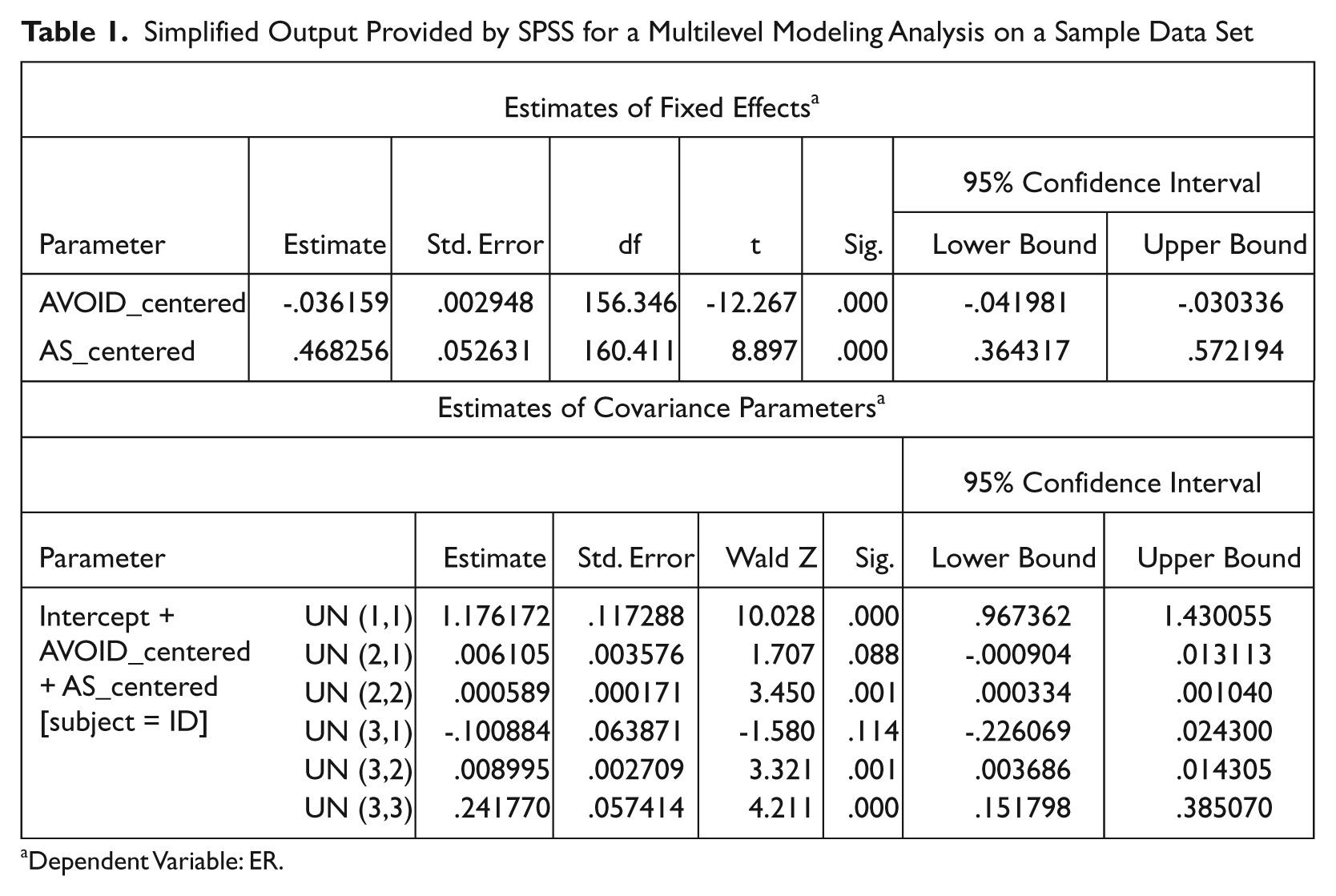
Dependent Variable: ER.
The second coefficient is a kind of variance on the previous coefficient and indicates whether the association between the explanatory variable and the outcome may be different for different people in the sample. The variance coefficient is provided in the “estimates of covariance parameters” table, in the row marked “UN (2,2).” (The coefficient for any additional Level 1 explanatory variables will be indicated by “UN (3,3),” “UN (4,4),” and so on; again, because Level 2 variables are not random, i.e., they do not vary from occasion to occasion, they will not have a variance provided.) It is helpful to convert this variance into a standard deviation (SD), which is easier to interpret. This must be done by hand, but recall that the standard deviation is the square root of the variance. The test of significance is provided on the same row as the coefficient. If it is significant, it means that the process relating the explanatory variable to the outcome is different for different people in terms of presence, direction, or magnitude. The larger the SD, the greater this variation. Because the unstandardized beta and the SD are in the same unit of measurement, comparing the magnitude of the SD to the beta it modifies gives an indication of just how wide this variation is. If the SD is larger than the beta, it suggests the association between explanatory variable and outcome may even be in the opposite direction for some people.
These are the steps to perform and interpret a basic MLM analysis using SPSS. Readers are referred to Fleeson (2007) for a more detailed discussion of the technique as well as problems that may be encountered. Following is an example of how to report and present findings from an MLM analysis, based on data from the example study on emotional reliance.
Reporting Multilevel Modeling in Methods and Results
Clarity is always important when describing how a statistical analysis was performed or when presenting the results of an analysis. Because MLM is still a relatively new procedure, there is sometimes a tendency to report more than is necessary or to include detailed formulas to specify the models that are being tested, much as it used to be customary to include full regression equations in studies that made use of regression techniques. Fleeson (2007), however, recommended using everyday language (e.g., referring to the results for “the typical individual” in the sample) and keeping tables as simple and uncluttered as possible. For a test of a basic MLM model, it is generally enough to report the unstandardized beta coefficient showing the association between explanatory variable and outcome for the typical individual and to report the standard deviation on this beta. (Of course, the test of significance for both should also be provided.) Following is an example of how the MLM analysis for the example study might be described in the Methods section and how the Results might be reported. For purposes of demonstration, here I will only test the association between emotional reliance and two Level 1 explanatory variables, attachment avoidance and autonomy support; the model tested in the original study (Lynch, 2012) is more complex.
Method (Example of How to Report)
Data Analytic Strategy
MLM was used to test the within-person process describing the relation between explanatory and outcome variables across four different relationship targets—mother, father, best friend, and romantic partner—in a sample of 247 undergraduate students. In addition, MLM provides a test of the possibility that between-person differences in the relationship between variables are not due to chance, denoted by the standard deviation on the main effect. MLM was conducted by means of the mixed models linear program in SPSS 18 (see Fleeson, 2007). The analysis tested the link between emotional reliance and attachment avoidance and autonomy support, with emotional reliance entered in the model as the dependent variable. The Level 1 explanatory variables, attachment avoidance and autonomy support, were mean-centered within each person to account for between-persons variance and ensure that results reflected the proposed within-person process.
Results (Example of How to Report)
The Process Relating Emotional Reliance to Attachment Avoidance and Autonomy Support
As shown in Table 2, unstandardized betas indicate that both the within-person Level 1 variables were significantly associated with emotional reliance: For the typical individual, there was a within-person process linking emotional reliance negatively with attachment avoidance and positively with autonomy support. Participants indicated greater willingness to turn to those partners with whom they experienced greater autonomy support but were less likely during an emotionally salient event to turn to those with whom they experienced an avoidant attachment. As previously noted, MLM provides a test of the possibility that the within-person process differed significantly across individuals. The results of this test, denoted by the standard deviations in Table 2, indicate that for both the within-person variables the process did differ across individuals: For some people, the association was stronger than for others. Comparing the magnitude of the standard deviation with that of the coefficient it modifies, for attachment avoidance the within-person process was in the same direction for each individual, but for autonomy support the association may even have been in the opposite direction for some individuals.
The Within-Person Process Relating Attachment Anxiety and Perceived Autonomy Support to Emotional Reliance
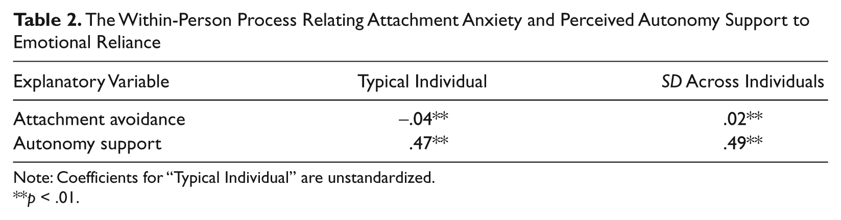
Note: Coefficients for “Typical Individual” are unstandardized.
p < .01.
Discussion
This section will address the issue of how counseling and developmental researchers might use MLM to address their own research questions.
Using Multilevel Modeling in Counseling and Developmental Research
The main purpose of the present article was to introduce researchers in counseling and human development to MLM, with the hope that a more user-friendly presentation might encourage them to consider using MLM to address their own research questions. Here I want to comment on how particular features of MLM may make it a particularly exciting analytic strategy for researchers in those fields.
MLM uses data that are hierarchically structured, that is, data in which observations at one level are nested within another level. This is important, because the kind of data that counseling researchers collect—or would like to collect—are often nested (Reise & Duan, 1999). For example, clients are often nested within some other unit, such as counselors, families, schools, agencies, and so on. MLM allows researchers to test how variations in some variable at the level of clients may be associated with variations in another variable at the level of counselors, and even allows for the possibility that the association between those variables may be different depending on the unit (here, counselor) within which clients happen to be nested.
Kahn (2011) described a number of published studies relevant to psychotherapy that used an MLM approach. His review provides a good starting point for how counseling researchers, in particular, might wish to apply MLM. A hypothetical test of the client–counselor relationship may serve as an illustrative example in the context of the present article. It is possible, for example, that client motivation may be linked to some aspect of the counselor’s way of being with the client, perhaps in terms of autonomy support (for a theoretical background of this argument, see Ryan, Lynch, Vansteenkiste, & Deci, 2011). If the autonomy supportiveness of, say, 20 counselors is measured, and the motivation of each counselor’s clients is also assessed, it might be possible to find not only that for the typical person autonomy support from the counselor is associated with more internal motivation for counseling in the client but also that the link between counselor autonomy support and client motivation is different from counselor to counselor. The source of such variation might be the focus of further study. Alternatively, if data collection for this hypothetical study were extended, and multiple observations for both clients and counselors were recorded over time, it might be possible to identify how client motivation fluctuates over time in relation to fluctuations in counselor style. As noted previously, this is a remarkable feature of MLM, in that it provides two kinds of coefficient: one testing the presence, strength, and direction of an association between variables (similar to the beta of a main effect in regression) and the other testing whether that association may be different for different people in the sample (the standard deviation on the first coefficient). This capability of MLM effectively frees quantitative researchers from the one-size-fits-all assumptions often embedded in regression analysis.
Developmental researchers also are often interested in data that are hierarchically structured. As noted earlier, MLM lends itself to an ecological framework, in which the person is embedded—or nested—within an ever-expanding series of contextual levels. It would be possible, for example, to design a study in which individual children are nested within families, with variables measured at both the child level and the family level. Alternatively, the study might look at families embedded within neighborhoods or at families embedded within cultural groups, and explore the association between variations in a variable measured at one level and variations in a variable measured at the other level. Features of both levels can be measured and included in the model, rather than treating one of the levels—culture, for example—as a kind of dummy variable. Importantly, MLM allows for the possibility that explanatory and outcome variables may be related to each other in different ways in different families, neighborhoods, or cultural groups.
Perhaps among the more intriguing capabilities of MLM for those in both counseling and development is its usefulness in studying longitudinal as well as within-person processes. In terms of studying variations or change over time, researchers might collect multiple assessments from the same participants over the course of weeks, months, or even years. In this case, observations are nested within individuals. If measures of both explanatory and outcome variables are collected at each assessment, it would be possible to test for within-person variations in the relationship between those variables, over time. Experience sampling is one way that nested data can be collected within individual participants over time, although experience sampling is typically used to study momentary variations rather than true developmental change (Fleeson, 2001, 2007); but other adaptations of the MLM approach for longitudinal studies are also possible (see, e.g., Francis, Fletcher, Stuebing, Davidson, & Thompson, 1991). The ability of MLM to test a proposed within-person process offers exciting possibilities for the counseling researcher, who might be interested, for example, in studying how momentary variations in perceived stress, or in perceived need satisfaction, map onto momentary variations in depressive symptoms, anxiety, and so on. If the data collected are hierarchically nested, with one unit of measurement embedded within another unit of measurement, the possibilities for using MLM to address questions in counseling and human development are limited only by the creativity and imagination of the researcher.
Footnotes
Appendix
Selected Data for 20 Participants Showing Autonomy Support (AS), Attachment Avoidance (AVOID), and Emotional Reliance (ER), Sorted by Participant ID and Relationship (RELP)
| ID | RELP | AS | AVOID | ER | AS_m | AVOID_m | AS_c | AVOID_c |
|---|---|---|---|---|---|---|---|---|
| 1 | 1 | 6.33 | 25.00 | 7.00 | 4.42 | 63.50 | 1.92 | −38.50 |
| 1 | 2 | 3.00 | 84.00 | 1.00 | 4.42 | 63.50 | −1.42 | 20.50 |
| 1 | 3 | 5.00 | 49.00 | 6.50 | 4.42 | 63.50 | 0.58 | −14.50 |
| 1 | 4 | 3.33 | 96.00 | 4.00 | 4.42 | 63.50 | −1.08 | 32.50 |
| 2 | 1 | 3.17 | 78.00 | 3.50 | 4.58 | 57.75 | −1.42 | 20.25 |
| 2 | 2 | 6.17 | 40.00 | 2.50 | 4.58 | 57.75 | 1.58 | −17.75 |
| 2 | 3 | 5.00 | 46.00 | 5.00 | 4.58 | 57.75 | 0.42 | −11.75 |
| 2 | 4 | 4.00 | 67.00 | 3.00 | 4.58 | 57.75 | −0.58 | 9.25 |
| 3 | 1 | 5.17 | 52.00 | 6.75 | 3.63 | 63.50 | 1.54 | −11.50 |
| 3 | 2 | 4.00 | 100.00 | 1.00 | 3.63 | 63.50 | 0.37 | 36.50 |
| 3 | 3 | 3.00 | 59.00 | 3.75 | 3.63 | 63.50 | −0.63 | −4.50 |
| 3 | 4 | 2.33 | 43.00 | 5.25 | 3.63 | 63.50 | −1.29 | −20.50 |
| 4 | 1 | 6.33 | 39.00 | 6.00 | 5.38 | 48.50 | 0.96 | −9.50 |
| 4 | 2 | 2.67 | 66.00 | 4.75 | 5.38 | 48.50 | −2.71 | 17.50 |
| 4 | 3 | 6.50 | 42.00 | 6.00 | 5.38 | 48.50 | 1.13 | −6.50 |
| 4 | 4 | 6.00 | 47.00 | 6.50 | 5.38 | 48.50 | 0.63 | −1.50 |
| 5 | 1 | 4.50 | 68.00 | 5.00 | 4.96 | 66.00 | −0.46 | 2.00 |
| 5 | 2 | 4.50 | 81.00 | 4.00 | 4.96 | 66.00 | −0.46 | 15.00 |
| 5 | 3 | 4.33 | 66.00 | 4.00 | 4.96 | 66.00 | −0.63 | .0 |
| 5 | 4 | 6.50 | 49.00 | 6.75 | 4.96 | 66.00 | 1.54 | −17.00 |
| 6 | 1 | 1.83 | 81.00 | 2.00 | 3.79 | 68.25 | −1.96 | 12.75 |
| 6 | 2 | 1.17 | 89.00 | 1.00 | 3.79 | 68.25 | −2.63 | 20.75 |
| 6 | 3 | 7.00 | 30.00 | 7.00 | 3.79 | 68.25 | 3.21 | −38.25 |
| 6 | 4 | 5.17 | 73.00 | 6.25 | 3.79 | 68.25 | 1.38 | 4.75 |
| 7 | 1 | 6.33 | 39.00 | 5.75 | 4.88 | 69.75 | 1.46 | −30.75 |
| 7 | 2 | 4.67 | 96.00 | 1.25 | 4.88 | 69.75 | −0.21 | 26.25 |
| 7 | 3 | 5.33 | 51.00 | 5.25 | 4.88 | 69.75 | 0.46 | −18.75 |
| 7 | 4 | 3.17 | 93.00 | 2.75 | 4.88 | 69.75 | −1.71 | 23.25 |
| 8 | 1 | 6.50 | 52.00 | 6.00 | 4.79 | 66.75 | 1.71 | −14.75 |
| 8 | 2 | 4.00 | 72.00 | 4.00 | 4.79 | 66.75 | −0.79 | 5.25 |
| 8 | 3 | 4.00 | 72.00 | 4.00 | 4.79 | 66.75 | −0.79 | 5.25 |
| 8 | 4 | 4.67 | 71.00 | 6.00 | 4.79 | 66.75 | −0.13 | 4.25 |
| 9 | 1 | 6.67 | 43.00 | 6.00 | 6.08 | 51.00 | 0.58 | −8.00 |
| 9 | 2 | 5.67 | 57.00 | 5.25 | 6.08 | 51.00 | −0.42 | 6.00 |
| 9 | 3 | 5.67 | 71.00 | 4.00 | 6.08 | 51.00 | −0.42 | 20.00 |
| 9 | 4 | 6.33 | 33.00 | 6.50 | 6.08 | 51.00 | 0.25 | −18.00 |
| 10 | 1 | 6.33 | 32.00 | 7.00 | 5.00 | 55.50 | 1.33 | −23.50 |
| 10 | 2 | 2.67 | 67.00 | 4.00 | 5.00 | 55.50 | −2.33 | 11.50 |
| 10 | 3 | 6.17 | 36.00 | 6.25 | 5.00 | 55.50 | 1.17 | −19.50 |
| 10 | 4 | 4.83 | 87.00 | 5.00 | 5.00 | 55.50 | −.17 | 31.50 |
| 11 | 1 | 6.67 | 41.00 | 6.25 | 6.21 | 43.00 | 0.46 | −2.00 |
| 11 | 2 | 5.83 | 39.00 | 7.00 | 6.21 | 43.00 | −0.38 | −4.00 |
| 11 | 3 | 7.00 | 28.00 | 6.75 | 6.21 | 43.00 | 0.79 | −15.00 |
| 11 | 4 | 5.33 | 64.00 | 6.00 | 6.21 | 43.00 | −0.88 | 21.00 |
| 12 | 1 | 5.17 | 43.00 | 5.25 | 5.50 | 46.25 | −0.33 | −3.25 |
| 12 | 2 | 4.50 | 54.00 | 3.25 | 5.50 | 46.25 | −1.00 | 7.75 |
| 12 | 3 | 5.83 | 41.00 | 5.00 | 5.50 | 46.25 | 0.33 | −5.25 |
| 12 | 4 | 6.50 | 47.00 | 7.00 | 5.50 | 46.25 | 1.00 | .75 |
| 13 | 1 | 6.83 | 25.00 | 7.00 | 6.00 | 36.75 | 0.83 | −11.75 |
| 13 | 2 | 5.67 | 39.00 | 7.00 | 6.00 | 36.75 | −0.33 | 2.25 |
| 13 | 3 | 5.83 | 43.00 | 6.00 | 6.00 | 36.75 | −0.17 | 6.25 |
| 13 | 4 | 5.67 | 40.00 | 7.00 | 6.00 | 36.75 | −0.33 | 3.25 |
| 14 | 1 | 5.00 | 49.00 | 7.00 | 5.42 | 62.75 | −0.42 | −13.75 |
| 14 | 2 | 7.00 | 61.00 | 7.00 | 5.42 | 62.75 | 1.58 | −1.75 |
| 14 | 3 | 4.83 | 65.00 | 4.75 | 5.42 | 62.75 | −0.58 | 2.25 |
| 14 | 4 | 4.83 | 76.00 | 5.00 | 5.42 | 62.75 | −0.58 | 13.25 |
| 15 | 1 | 6.33 | 29.00 | 7.00 | 4.13 | 60.00 | 2.21 | −31.00 |
| 15 | 2 | 2.00 | 111.00 | 1.00 | 4.13 | 60.00 | −2.13 | 51.00 |
| 15 | 3 | 5.50 | 51.00 | 5.00 | 4.13 | 60.00 | 1.38 | −9.00 |
| 15 | 4 | 2.67 | 49.00 | 7.00 | 4.13 | 60.00 | −1.46 | −11.00 |
| 16 | 1 | 1.50 | 92.00 | 2.00 | 4.17 | 53.00 | −2.67 | 39.00 |
| 16 | 2 | 2.33 | 70.00 | 4.25 | 4.17 | 53.00 | −1.83 | 17.00 |
| 16 | 3 | 6.17 | 25.00 | 6.25 | 4.17 | 53.00 | 2.00 | −28.00 |
| 16 | 4 | 6.67 | 25.00 | 7.00 | 4.17 | 53.00 | 2.50 | −28.00 |
| 17 | 1 | 7.00 | 24.00 | 7.00 | 6.88 | 37.75 | 0.13 | −13.75 |
| 17 | 2 | 6.83 | 26.00 | 7.00 | 6.88 | 37.75 | −0.04 | −11.75 |
| 17 | 3 | 7.00 | 24.00 | 7.00 | 6.88 | 37.75 | 0.13 | −13.75 |
| 17 | 4 | 6.67 | 77.00 | 6.00 | 6.88 | 37.75 | −0.21 | 39.25 |
| 18 | 1 | 4.33 | 51.00 | 4.25 | 4.67 | 53.50 | −0.33 | −2.50 |
| 18 | 2 | 3.67 | 72.00 | 2.75 | 4.67 | 53.50 | −1.00 | 18.50 |
| 18 | 3 | 5.17 | 50.00 | 5.00 | 4.67 | 53.50 | 0.50 | −3.50 |
| 18 | 4 | 5.50 | 41.00 | 6.00 | 4.67 | 53.50 | 0.83 | −12.50 |
| 19 | 1 | 5.33 | 68.00 | 4.00 | 4.58 | 66.25 | 0.75 | 1.75 |
| 19 | 2 | 4.00 | 72.00 | 4.00 | 4.58 | 66.25 | −0.58 | 5.75 |
| 19 | 3 | 4.00 | 72.00 | 4.00 | 4.58 | 66.25 | −0.58 | 5.75 |
| 19 | 4 | 5.00 | 53.00 | 4.50 | 4.58 | 66.25 | 0.42 | −13.25 |
| 20 | 1 | 6.50 | 26.00 | 7.00 | 5.54 | 47.50 | 0.96 | −21.50 |
| 20 | 2 | 4.83 | 71.00 | 4.25 | 5.54 | 47.50 | −0.71 | 23.50 |
| 20 | 3 | 6.00 | 42.00 | 5.75 | 5.54 | 47.50 | 0.46 | −5.50 |
| 20 | 4 | 4.83 | 51.00 | 5.25 | 5.54 | 47.50 | −0.71 | 3.50 |

Note: The subscripts, “_m” and “_c,” refer to mean and centered values, respectively.
The author(s) declared no potential conflicts of interest with respect to the research, authorship, and/or publication of this article.
The author(s) received no financial support for the research, authorship, and/or publication of this article.