
Abstract
This review presents a conceptual model to understand and trace the effects of land development on municipal expenditures and revenues. It includes discussion of the how local voters determine levels of expenditures and levels of service subject to external constraints. It also discusses the production function of local public services. This review and model can serve as a basis for evaluating fiscal projections for land development proposals. It finds that direct fiscal impacts measured in most fiscal impact analysis techniques are only a subset of the types of impacts that would likely be expected to result from land development within a community.
Introduction
Land development impacts local public finance because development (or redevelopment) generates changes in the levels of service (LOS) or quality of services demanded, attracts new residents who may have different demographic and service demands than existing residents, and generates changes in revenues. Forecasting (and mitigating) the magnitude and direction of these revenue and expenditure changes has become an important, if not central, concern for local governments (Gottlieb 2006; Wassmer 2002; Lewis 2001). Many critics have even suggested that fiscal considerations have come to play too dominant a role in local government land use decision making (Bunnell 1997; Lewis 2001; Wassmer 2002).
Fiscal impact projection and analysis techniques claim to be able to estimate changes in revenues and expenditures likely to result from land development within a jurisdiction. In order for fiscal analyses to provide accurate, reliable, and usable information for local government policy and land use decisions, models, and methods utilize some assumptions (either explicitly or implicitly) of the mechanisms linking land use change with service demands, revenues, and expenditures. In practice, most fiscal impact analyses prepared for local governments utilize strong assumptions regarding the mechanism between land development and fiscal outcomes. Local fiscal projections face trade-offs between analytical tractability, simplicity, and limitations of the projection method. The limitations and assumptions of fiscal impact projections may not always be explicitly stated, which may give local decision makers a false certainty about the precision of the estimates. Even though some of the earliest research on fiscal methodologies (Burchell and Listokin 1978) warns users both to understand the assumptions and limitations of the techniques and not to use fiscal analyses as the primary basis for excluding or promoting certain developments, these warnings have not usually been heeded in practice (Edwards and Huddleston 2010).
The purpose of this review is to offer a conceptual understanding of the processes linking land use change to local fiscal change. This review provides a framework for understanding and evaluating the use of fiscal projection techniques in land use decision making and identifies existing gaps in knowledge and research. Because analysis of the fiscal impacts of land development requires making assumptions about how local governments raise and spend public dollars, and also how land development alters this relationship, the purpose of this article is to organize the extant empirical and theoretical research into a coherent and comprehensive understanding of the effects of land use change on local government revenues and expenditure patterns. This review is based on a wide body of research across multiple fields, and arenas for future possible research are suggested. Despite the wide range of research in this field, some of the basic relationships between land development and municipal finance remain poorly understood.
While fiscal impact analyses, cost–revenue analyses (Wheaton 1959), or costs-of-community-services analyses have existed for decades to help local governments make short- and long-term land use and infrastructure decisions (Schaenman and Muller 1974), they have become much more widespread in the planning profession in recent years (Edwards and Huddleston 2010). There are at least two reasons for more widespread adoption of fiscal projection techniques in connection with land development decisions at the local level. First is the publication and widespread availability of standardized workbooks and spreadsheets, beginning with Burchell and Listokin’s (1978) seminal (and later revisions) workbooks (Burchell, Listokin, and Dolphin 1985, 1994; Burchell and Listokin 1991, 1980, 1978). With these workbooks, even small communities without dedicated fiscal staff could utilize methods and multipliers to make reasonable first-order projections of fiscal impacts. Second, the decline in federal assistance to local communities for infrastructure and revenue sharing (Fisher 2003) has forced local governments to deal with the infrastructure and service requirements of new growth. In the present economic downturn, the decline in state aid to local governments has further tightened the fiscal environment for local governments (Zhao and Coyne 2011).
The method used for this research was literature searches of published articles and books in the planning, public administration, public finance, and economics literatures, using key words (and all linguistic variants) “fiscal,” “local” “municipal,” “public finance,” “land development,” “fiscal impact,” “median voter,” and the like. One contribution of this article to planning knowledge and scholarship is the incorporation of economics and public administration disciplines. In addition, contents of a number of specific journals were reviewed for the previous twenty years: Journal of Public Economics, National Tax Journal, Public Budgeting and Finance, Public Finance Quarterly/Public Finance Review. Academic and published research was used, including working papers produced by the National Bureau of Economic Research and the various Federal Reserve Banks. Studies were limited to the US context because of its reasonably unique localism in land use and fiscal federalism. Research was limited to academically oriented publications and materials and therefore was not able to include most of the practitioner-oriented material available.
This article is organized as follows. Figure 1 both represents the conceptual “model” of fiscal analysis used in this research and serves as road map of the argument. First, an outline of what an “initial equilibrium” in a community (representing a “status quo” prior to land development) might look like is presented. This heuristic concept of equilibrium is used as a framework to think about the interrelationships of existing patterns of land development and existing patterns of revenues and expenditures. Discussion here focuses on expenditures, detailing the process of local public expenditure determination. Observed differences in expenditures across cities result from differences in voters’ public service demands, the production function of local public goods, the regional context, and intergovernmental relations. This article will treat each in order. Second, two prototype land developments are examined and the likely effects of these developments on a city’s expenditures and revenues are traced through the model, highlighting areas where existing empirical research provides some certainty and areas where research does not. This discussion highlights the fact that most fiscal analysis techniques only deal with the likely “direct” fiscal impacts (shown as the shaded area of Figure 1) but not with the likely “indirect” impacts. Areas of potential research to improve understanding of and projections of the impacts of development are presented, along with discussion of implications for planning practice.
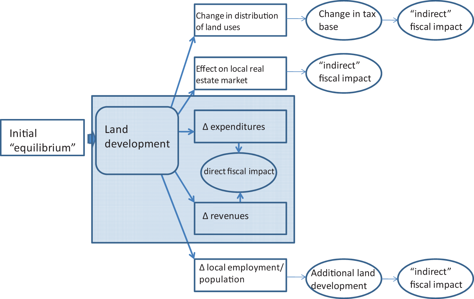
Conceptual “road map” of land development and fiscal change.
Characterizing Initial Equilibrium
The conceptual model for understanding fiscal impacts presented in Figure 1 begins with a heuristic of “equilibrium” prior to the changes induced by a land development. The concept of “equilibrium” is used as a way to exposit the underlying relationships between land development, revenues, and expenditures. Within the economics literature, the idea of equilibrium is where resources and prices have adjusted to some balanced state in response to a shock. Equilibrium conditions do not necessarily need to be identified or proven for the concept of equilibrium to be useful for exposition. Likewise, the concept of “equilibrium” in chemical or natural systems connotes a system in balance. It is only in this sense that the term is used, merely as a heuristic or expository device, and not as any larger claim about the existence or nature of such equilibrium. This is because many researchers within the field of local public finance have pointed out that there does not exist (yet) anything like a fully generalizable, empirically tractable equilibrium model of the local public sector which encompasses land development and housing markets. Many have even questioned whether such stable equilibria exist (Hanushek 2002; Ross and Yinger 1999; Nechyba and Strauss 1998).
The purpose of thinking about initial equilibrium is to identify the structural forces and relationships in the existing pattern of revenues and expenditures. Then, one can imagine a “shock” to the system in the form of a land development within a city. Changes in revenues and expenditures can then be traced through the system in response to land development. Revenues, expenditures, public service demands, and real estate values all change in response to the land development, eventually adjusting to some equilibrium. At the most general level of thinking, differences in expenditures and revenues from the initial equilibrium to the new equilibrium reflect the “fiscal” impact of the land development.
For purposes of organizing this review, start by considering a city in equilibrium with some existing level of land development, expenditures, revenues, and residents. This observed pattern of land use, expenditures, and revenues would reflect the decisions of and prior interactions of a large number of independent actors over time, as constrained by the legal, economic, political, and institutional structure unique to each city and state. Discussion below begins with the process of expenditure determination as a function of service demands and external constraints, with additional focus on the production function of local public goods.
Expenditures
Understanding how local expenditures are determined is actually one of the most crucial assumptions in any fiscal analysis. In practice, most local fiscal analyses make quite strong assumptions about the expenditure determination process. These assumptions can often imply a level of certainty about the likely changes to expenditures from land development. Such certainty, however, is not necessarily consistent with the empirical and theoretical literature reviewed here. In order to evaluate the use of fiscal methods and to suggest areas for improvement and research, it is necessary to take a detailed look at the literature on local expenditure determination.
Local governments in the United States, based on the 2009 Census of Government Finances, undertake direct expenditures of US$1.6 trillion per year. These local governments (counties, municipalities, school districts, and special districts such as sewer and water authorities, transit operators, etc.) spend money to provide a wide range of public services and public service responsibilities vary from state to state. Of this US$1.6 trillion, the most (37 percent) is spent on education, with social services, public safety, and environmental services (parks, natural resources, water, sewerage, etc.) in descending order of expenditure shares. These data confirm general public perceptions that local governments mostly provide basic public services such as public education, public health, parks, water and sewer, and public safety. Therefore, all of the examples used in this article will focus on these basic public services.
At the beginning of the discussion, however, and to clear up a common confusion in research and planning practice, it is important to distinguish between “costs” and “expenditures.” While these terms are often used interchangeably, this verbal confusion can introduce imprecise thinking among planners and local policy makers. As has been repeatedly pointed out over the years (see, e.g., Ladd, 1994, 1998), there simply is not any good or reliable data on local government public service costs. The data that are available is on expenditures. Expenditures represent the number of units of a particular service provided multiplied by the cost-per-service unit. Differences across places in the levels of expenditure may reflect differences in costs, but can also reflect differences in the number of service units provided or the LOS provided. A priori, there is actually no way to use expenditure data to infer anything about costs. Using differences in expenditure data to infer differences in costs across places is, therefore, incorrect. The LOS provided in a community reflects residents’ demand for services, itself a function of demographics and income.
To illustrate, consider two communities. Community 1 spends US$500 more per capita on education or public safety than community 2. This observation does not provide any information about cost differentials between community 1 and community 2. It might be the case that voters in community 1 prefer a higher LOS than community 2’s voters. Even if there are identical per unit costs, expenditures in community 1 could be higher than in community 2 to reflect these different LOS. Perhaps community 1 prefers smaller class sizes or more police officers. Alternatively, it could be the case that voters in communities 1 and 2 both desire the same LOS, but wage and benefits costs per public employee in community 1 are higher than in community 2. To employ the same number of teachers or police officers, community 1 would have higher “costs” and therefore higher expenditures. It is also possible that community 1 is experiencing a higher crime rate or has more children in need of more specialized educational assistance, driving higher levels of expenditure even if per unit service costs are the same. It is even possible that one community could have a higher level of expenditures per capita but have an outcome-based LOS (such as crime rate or test scores) which is lower than surrounding communities.
One example of this conceptual confusion is seen in some of “costs of sprawl” literature, which takes the positive correlation between sprawl and expenditure as implying that public service costs are higher in more sprawling places. But expenditure data alone cannot tell us whether more sprawling places have higher costs or whether this higher level of expenditure reflects higher incomes. Public service demand, as discussed below, is known to be income elastic and should therefore result in higher expenditures in higher-income communities. Similarly, the types of fiscal studies called costs of community services can be misleading because the data used to construct such studies is actually expenditure data, not cost data.
One area with substantial empirical work in local public finance concerns police expenditures (see, e.g., Zhao, Ren, and Lovrich 2010) which can illustrate the distinctions between expenditures and costs. Local voters who control the expenditure determination process have a demand for a certain level of “public safety”—which is really the experience of being safe from crime. If one could have access to detailed police department accounting data, it might be possible to measure input prices or “costs” in terms of police employee wages and benefits, capital and current costs of buildings, patrol cars, fuel, materials and supplies, and so on. Labor input ratios such as number of police officers per capita, as well as outputs such as number of patrols, response rates, arrest rates, and case clearance rates could be measured. Outcomes such as the crime rate or insured losses to property could be measured as well. Generally, however, across jurisdictions or even across time within a jurisdiction there is only data on actual police expenditures. One municipality may spend more per capita on police because it is adjacent to a higher crime area and needs to spend more to produce a desired level of the “public safety” outcome. Another municipality may spend more on police per capita because its costs per labor input are higher. Yet another municipality may spend more on police per capita because it is a wealthy community with a low-crime rate, but public safety is an income elastic public good and higher-income residents pressure their community to produce high levels of safety. Two communities may spend the exact same amount on police and have the same crime rate, while one community faces higher wage costs and thus uses more technology per officer or fewer neighborhood patrols, while the other community uses more officers on the streets.
In practice, most fiscal impact analyses have not made clear this distinction between costs and expenditures. Many off-the-shelf fiscal projection tools use what is often called the average cost method, which is in reality an “average expenditure” method. In a survey of planning directors as to which fiscal techniques are more commonly used, Edwards and Huddleston (2010) do report that the case study (marginal cost) technique is used most often. The case study technique comes closest to representing the distinction between costs and expenditures because the method usually involves the analyst requesting detailed cost and budget information from relevant departments within the city. Certainly, one implication for practice of this current discussion is that analysts should clearly specify to what extent projected expenditure changes are based on assumptions of changes in per unit costs or changes in the number of service units to be provided. Even when assumptions are explicitly stated, local fiscal analyses require strong assumptions about the process of expenditure determination.
What determines the level of expenditure within a community? As a general statement to represent empirical and theoretical literatures, local voters, subject to external constraints, chose that level of expenditures which will produce the desired LOS, conditional on having to pay for expenditures through tax revenues. Each of these three components (local voters’ service demands, external constraints, and the production function of local public services) will be discussed in order below. For purposes of this review and in keeping with much of the empirical literature, it is assumed that expenditure decisions largely reflect the demand side of public services and are independent of structural factor on the revenue side. This assumption may not necessarily be true for two reasons. First, there is some evidence that different revenue shares (percentage from property tax, sales tax, and/or income tax) could influence expenditure levels (Gill and Haurin 2001). Second, there is some evidence that the “tax price” of public expenditures for local voters could influence expenditure levels. The “tax price” of public expenditures is the cost to local voters of an additional US$1 in public expenditure. Depending on the structure of local revenues, local voters may pay less than US$1 to raise US$1 in revenue. Consider a simple case where only property taxes fund local revenues and in a state with a uniformity provision for property taxation (nonexempt property must be taxed at a uniform rate regardless of classification). If 30 percent of the tax base is commercial/industrial property, then residential taxpayer-voters would only see a “tax-price” of US$0.70 for US$1 in additional expenditure. This lower “tax-price” might induce voters to chose a higher level of expenditure than if they had to pay the full cost (Ladd 1998). Of course, voters would understand that there are constraints on overtaxing the businesses within their community because capital is mobile and jurisdictions compete for desirable property tax bases (Gottlieb 2006). The analysis of the “tax price” faced by local voters would be more complicated in cases of differential taxation and/or property tax exemptions, but the principle is the same.
The empirical and theoretical literature on the determinants of expenditures in local governments is often called the expenditure demand literature (Bradbury and Stephenson 2003; Bradbury, Mayer, and Case 2001; Ladd 1998; Merrifield 2000; Shadbegian 1998; Sjoquist, Walker, and Wallace 2005).
These studies use the analytic technique of consumer demand studies with the assumption that household sorting into communities based on preferences serves as a “demand” or “preference” revelation mechanism (Tiebout 1956). Households’ demand for local public services should approximate the LOS offered in their community, or they would move to a different community more closely matching their demand for services. Thus, the level of expenditure within a community should reflect the demand characteristics of its population, and the empirical proxies for these demand characteristics are socioeconomic and demographic characteristics of the population. Beginning with pioneering studies in the early 1970s (Bergstrom, Rubinfeld, and Shapiro 1982; Bergstrom and Goodman 1973; Borcherding and Deacon 1972), local public goods have been studied using this consumer demand framework. Empirically, local public goods have been found to exhibit more of the characteristics of private goods (particularly congestability and rivalry in consumption) than of “pure” public goods, which lends credence to analyzing the demand for local public goods within a consumer demand framework. The concept of “demand” for local public goods is not, however, without controversy, given that welfare and equity considerations are involved in local public goods, particularly education and public safety. Many people, including many planners, think these goods (education, public safety, health, etc.) should be treated as “merit” goods rather than “benefit” goods. This controversy is raised to broaden the discussion of local public expenditure, but dealing with the equity implications of local public goods demand is beyond the scope of this review (Chakravorty 1999).
Voters’ Service Demands
Although visitors to a city and nonresidential property both impose service demands on cities (Nelson 2004), most research understands public expenditures to reflect either the demand characteristics of resident voters or the demand characteristics associated with organized and influential interest groups within the community. The various “voter” models of public expenditure determination are based on the idea that local public officials offer that level of public expenditures and revenues (revenue–expenditure bundles) which maximizes the probability of securing approval from the voters. Whether the form of local government is representative or entails direct democracy provisions such as referenda for capital expenditures, officials who offer levels of expenditure too high or too low will soon be replaced with other elected officials. The discipline of voting, along with household mobility and capital mobility, is thought to lead to expenditure and service levels which closely reflect voters’ demands.
Within voter models of local public expenditure, there are two dominant variants: the median-voter model and the interest group model. Like other disputes in empirical public finance, these models continue to generate a large literature which has not achieved anything like a consensus (Brunner and Ross 2010; Chandler 2005). The median-voter model argues that the demand characteristics of the median voter prevail in local expenditure decisions because local officials compete to offer the revenue–expenditure bundle preferred by the median voter. Public officials who do not offer the bundle which satisfies the demand of the median voter are soon voted out of office, or may find that bundle voted down in a referendum. The median-voter model has dominated much of the local public finance economics and urban economics literatures for much of the last forty years, especially given the dominant position of Tieboutian sorting as a model of local public goods demand revelation (Fischel 1992; Howell-Moroney 2008; Nechyba 2007; Ross and Yinger 1999; Voith and Gyourko 2002; Wheaton 1993). In empirical implementation, much of the work in this field assumes that the median voter is the voter with the median income, an assumption that has more recently been challenged (Brunner and Ross 2010).
The alternative approach is to argue that organized stakeholder groups are able to influence expenditure determination away from what the median resident would desire, either through insider knowledge of the political process or through organized mobilization. The interest groups identified as exercising strong influence on local expenditure levels have included “budget maximizing bureaucrats,” public sector unions, homeowners, and renters. In the “bureaucracy” model, also called the Leviathan model (Park, McCabe, and Feiock 2010; Brunner and Ross 2010), local governments are dominated by public sector unions or bureaucrats who want to keep levels of expenditure higher than what the median voter would prefer. If policy makers or voters believe the bureaucracy model to be correct, then they are more likely to press for policies such as revenue caps, expenditure caps, assessment caps, and so on—collectively called tax and expenditure limitations (TELs; McGuire 1999; Mullins 2004; Deller and Maher 2005; Shadbegian 1998; Hoyt 1999; Dye and McGuire 1997). In fact, the widespread presence of TELs (following Proposition 13) is taken as prima facie evidence that voters believe the bureaucracy model is at least partially correct and that external rules need to be imposed on local government decision makers to constrain expenditure growth (McGuire 1999).
Other versions of the interest-group model of local expenditure determination focus on homeowner-voters (whom Fischel famously termed “homevoters”) or renters. Oates (2005) presents a meta-analysis of studies to test for the “renter effect” (the idea that renters vote for higher levels of expenditure because they do not directly pay the property tax) and uses multiple data sets to estimate a renter effect of 10 percent. By this he means that, on average, local public expenditures are 10 percent higher than they would otherwise be in a situation of 100 percent homeownership. However, in more recent empirical work, Banzhaf and Oates (2012) find no evidence of a “renter effect” in terms of specific voting for open-space referenda. This may be because, while renters can enjoy parks and open-space amenities on equal terms with homeowners, they do not experience the property value impacts of open-space preservation on nearby properties. As Schmidt and Paulsen (2009) demonstrate, homeowner-voters are more likely to vote to preserve open spaces to protect and enhance their own property values. Moreover, Schwab and Zampelli (1987) find no statistically significant “renter effect” in public safety expenditures.
For economists, the basic idea behind a “renter effect” is some type of “illusion” where renters vote for higher levels of public expenditure because they do not directly pay for these expenditures with property taxes, even though property taxes are capitalized into land values and hence rents (Krueckeberg 1999) if not always completely (Carroll and Yinger 1994). Quoting Oates (2005), “There is little reason to expect the renter effect to reflect a systematically higher level of demand for public services by renters … [because] the demands of renters, if anything, are likely to be lower than those of home-owners, since renters have, on average, lower incomes and smaller family-size. The most obvious and plausible explanation is that renters support larger local budgets because they don’t think they cost them much (if anything). From this perspective, we can reasonably regard the renter effect as representing excessive public spending” (p. 427). Despite the persistence of the “renter effect” in empirical work, there is little consensus as to the cause or the meaning of the effect. Why does the effect exist at all, given that renters have much lower voting participation rates than do homeowners, especially in local races or referenda (Holian 2011) and that so many communities impose multiple restrictions upon construction of rental housing (Paulsen 2012b; Schuetz 2009)?
Fischel’s (2001a, 2004) “homevoter hypothesis” in its most basic form argues that risk-averse homeowners, perhaps the most dominant interest group in local politics, jointly monitor local land use and spending decisions and vote for both expenditure levels and zoning restrictions to protect and maximize their property values. Restrictive land development regulations are promoted by homeowners not only to restrict overall development (scarcity effect) but also to limit or exclude land developments which could cause expenditures to be higher than homeowners would desire (public goods effect). This theory is a dynamic theory of local public finance, and one which needs to be understood carefully. It is less of a voting model than it is a choosing-future-voters-in-our-city model. The homeowners in Fischel’s model are not only “homevoters” but are really “homevoterzoners”—homeowners who vote in local elections to control zoning in order to protect the value of their largest (and undiversifiable) asset, their home. The “renter effect” and “homevoter hypothesis” are not necessarily contradictory understandings of local land development and public finance, at least when viewed dynamically. If homeowners believe the “renter effect” in local expenditures to be real, they have a fiscal incentive to reduce the possibility of lands made available for rental housing construction (Fischel 1992; Schuetz 2008, 2009) or reduce the number of bedrooms in rental units to limit the potential fiscal impact of additional schoolchildren (Paulsen 2012b). Within the language of the sorting-and-voting public finance models (Ross and Yinger 1999), the disconnect is that the marginal housing consumer in a community (homebuyer or renter) is likely not the median voter. Thus, the “fiscal” basis of exclusionary zoning (James and Windsor 1976; Bogart 1993; Paulsen 2006; Ihlanfeldt 2004).
These questions of public expenditure determination are not merely an arena for academic theorizing and empirical analysis. Even if these relationships are obscured in fiscal analyses, local voters and local elected officials must believe some implicit causal model of the relationships between land development and expenditures. Land development brings new residents into the community. These new residents have potentially different demographic correlates and different service demands, potentially altering who the median voter is. When existing residents try to block certain types of land developments for fiscal reasons, they are not only concerned with additional service demand units but are also concerned that future residents may have demands for expenditures which differ from those of established residents. If, to take a controversial example, lower-income rental housing is proposed in a community, existing homeowners not only make the fiscal impact argument (that rental housing brings in less revenue than it “costs” in expenditures) but implicitly argue that lower-income renters alter the median voter’s desired level of expenditures.
External Constraints
The two broad categories of external constraints on local public expenditures are mobility (of household and capital) and intergovernmental relations. Cities compete for both mobile households and mobile capital, which can potentially move to another jurisdiction if service levels or tax rates or land use regulations are undesirable. In the same way that market competition is thought to discipline firms toward efficiency and competition on quality or price, competition between cities for mobile households and mobile capital is thought to discipline land development and expenditure decisions to reflect demand characteristics efficiently. And, consistent with this idea, standard public finance models assume that mobile households and mobile capital limit the ability of local governments to engage in redistribution (Fisher 2003; Fisher and Wassmer 1998; Ladd 1994).
Household mobility has been the key mechanism of “urban public finance” models—where sorting through the housing market, land development decisions, and voting for local public expenditures are all jointly determined (Ross and Yinger 1999; Tiebout 1956). When households purchase a housing unit, they also “purchase” the local public goods attached to that house, including neighborhood amenities and locationally conditioned public services like schools and public safety. Because households have a number of different communities to choose from within a metropolitan area, they are able to “shop” or “vote with their feet” for that community with the mix of taxes and expenditures which most closely approximates their demand for public goods (Fischel 2000; Heikkila 1996; Tiebout 1956). Household sorting as an expenditure demand revelation mechanism is complicated by the fact that households also have preferences for the socioeconomic, demographic, and racial characteristics of their neighbors (Dawkins 2005, 2006).
Just as household mobility constrains local fiscal policy, so too does capital mobility. Businesses and real estate developers can choose from a number of communities in which to invest, and thus municipalities compete to attract businesses through lower tax rates, special tax incentives, and/or solicitous land use and zoning regulations. If taxes in one municipality become too high, businesses can move. Capital mobility suggests that business tax rates will be kept low as municipalities compete for mobile capital. And, as above, because a larger commercial/industrial tax base reduces the “tax price” residents face for public expenditures, local regulations are often described as serving to compete for “fiscally” desirable land uses, also called ratable chasing (Gottlieb 2006).
The second area of constraints on voters’ decisions is intergovernmental relations, which includes competition with neighboring jurisdictions and relations with state governments. Local governments compete with one another for households and land uses which generate desirable tax bases or a “fiscal surplus” (Alesina, Baqir, and Hoxby 2004; Bayer, McMillan, and Rueben 2004; Bell et al. 2004; Bradbury and Stephenson 2003; Brueckner 1999; Gottlieb 2006; Heikkila 1996; Ross and Yinger 1999; Wassmer 2002). When land uses generate a “fiscal surplus” (such as office parks or auto dealerships), developers can seek the community offering the most concessionary terms or incentives. Local governments compete with one another through tax exemptions, infrastructure projects, tax increment financing expenditures, and the like.
Decisions of nearby local governments can have tremendous influence on the land use and public finance patterns of other local governments. Competition among municipalities in the form of “ratable chasing” behavior has been shown to exert a significant impact on land use and finance decisions (Gottlieb 2006). Land use and public finance decisions in one community can have significant spillover effects on neighboring communities, including traffic congestion or changing demand for housing. However, it is not standard practice in fiscal impact analysis for communities to project or consider the likely impacts on neighbors or to consider the likely fiscal impact to their own communities of development in neighboring communities.
Perhaps more than any other feature of the local land-use-and-fiscal system, competition among own-source-revenue-dependent local governments for mobile households and mobile capital—“competitive fiscal federalism”—distinguishes American local governance from that of other countries (Oates 1999, 2001; Ladd 1998). The combination of interjurisdictional competition, capital and household mobility, and dependence on the property tax to fund local public goods necessitates local concern about the fiscal impacts of land development.
In the literature which evaluates this system, some view this competition as necessary to produce efficiency (Paretian, not technical) in local land use and tax policies (Howell-Moroney 2008; Nechyba 2007; Wheaton 1993; Fischel 1992; Wassmer and Fisher 2000; Ladd 1998). However, other scholars find that competition and fragmentation of local governance of land use and public goods produces perverse incentives which help generate many of the undesirable characteristics of metropolitan spatial patterns (sprawl, racial segregation, fiscal and economic disparities, etc.; Heikkila 1996; Howell-Moroney 2008; Ladd 1999; Ladd and Yinger 1991; Paulsen 2006; Rhode and Strumpf 2002).
Competitive fiscal federalism makes local fiscal analyses of land development necessary, but also renders most analyses problematic. Projections of likely fiscal impacts for one community almost never consider the fiscal, land use, and other indirect impacts on neighboring jurisdictions. Moreover, it is just as likely to be the case that competition and dynamic adjustment by households and businesses may compete away any projected “fiscal surplus” of a particular development. One canonical example illustrates this point. A fiscal analysis of a new shopping center in a community could show a “fiscal surplus” for the development based on standard linear projections of direct revenues and expenditures. However, if the new shopping center draws customers and property value away from existing commercial land uses within the city (or the region at large), the reduced property value, employment and therefore revenues from existing commercial development may result in no net fiscal surplus for the community over time.
The second area of intergovernmental relations which constrains local voters is relations with the state government. State governments through enabling legislation, home rule charter provisions, court decisions, and budgetary decisions determine the structure of local government finance and land use, which vary substantially from state to state. State governments assign functional service provision requirements and obligations to different levels of local government. In some states, local governments manage tax assessments or provide public health and welfare services, while in other states these are county responsibilities. State enabling legislation defines the types of taxes local governments may, may not, or must collect, with specifications as to the composition of the tax base, tax rates, and various exemptions, exclusions, deductions, and credits. In some states, local governments are enabled to levy local option income taxes, and other states allow local governments to collect a portion of in situ sales taxes. Some states allow for discretionary tax abatements, while others do not. States specify the terms and conditions of public employment, particularly in requirements for public employee bargaining, compensation, and benefits. Because public employee wages and benefits constitute a substantial portion of local government budgets, these state rules significantly impact local expenditure levels.
Some states also impose TELs, or supermajority and/or referenda requirements on local government expenditures, particularly for capital projects or debt issuance. These external constraints on local fiscal decision making structure the effects of land development on actual fiscal outcomes. Understanding the decision-making structure of local governments under TELs or supermajority requirements has frequently been difficult, and has often been treated inconsistently by many fiscal analysts. As an example, consider the case where a large land development generates revenues or expenditures which could cause a local government to exceed its revenue or expenditure caps. In such a case, the marginal impact of that land development would be different in one community than in another community further away from their cap.
State governments also significantly impact local finance through revenue sharing, grants, school aids, and equalization formulae (Mieszkowski and Musgrave 1999; Hoxby 2001). Outside-source revenues can play an important role in local government budgets, and therefore significantly alter land use and fiscal decisions. Fiscal analyses of local governments should pay careful attention to the structure of outside-source revenues, including projections of the likely impact of land development proposals on outside-source revenues. One area of great difficulty for local fiscal analysis has been projecting the impacts of a land development on state aids or equalization grants when state formulae depend on property tax-based fiscal capacity and fiscal effort. For example, while a large nonresidential development may appear to add to the tax base of a community without an increase in schoolchildren, this increase in the tax base per student may cause a school districts’ equalization aid from the state to decline (Gottlieb 2006; Huddleston 2009).
LOS and the Production Function of Local Public Goods
Before examining the likely effects of land development on local finance, it is necessary here to “open the hood” and examine in greater detail the production function of local public goods. If voter preferences represent the “demand” side of local services, the production function can be thought to represent the “supply” side.
The mechanisms by which public sector services are translated from public sector inputs into outputs and outcomes is complex, and this complexity is often obscured in the assumptions and simplifications necessary to produce fiscal impact analyses in a jurisdiction. Yet, it is important to get behind this complexity by attempting to draw out a more fully specified model or understanding of the nature of public goods provision and service level outcomes from the literature. When this complexity is explored, it turns out there is little that can actually be said a priori about the expected effects of land development on public finance, absent strong assumptions. Because fiscal analysis techniques are designed to inform local residents and policy makers about the likely consequences of land development, the assumptions used in developing projections should be made more explicit. While it is unrealistic and impracticable to assume that every fiscal impact analysis must specifically address all of the factors identified here, the conceptual model presented here can serve as a template or benchmark against with to evaluate fiscal impact analysis techniques.
Within a more general economics literature, the term production function is used to describe the underlying technological relationships by which firms translate “inputs” (labor, capital, energy, materials, etc.) into “outputs.” Firms make decisions (maximizing profit and minimizing cost) based on the interaction between their technologies, factor input prices, and output prices. The concept of a production function has been used as a helpful heuristic in understanding local government service provision, but not without some complications (Schwartz 1993). Traditional production analysis focuses on firms’ “outputs” but for local public services what local voters really care about is “outcomes” such as uncongested streets, well-maintained and accessible parks, low crime rates, high test scores, and so on. These outcomes are the end result of a complicated process of local public service delivery interacting with the characteristics of the population.
It is important to emphasize again that observed patterns of expenditures will be a combination both of voters’ desired level of public service and the underlying “production function” by which local governments transform inputs into desirable public service outcomes. A high level of expenditures in a municipality may reflect either high LOS demand, high per unit costs, or both. It is not possible to understand the observed relationship between land use and expenditure patterns without understanding how these two interact (service-level determination and the production function).
The concept of “LOS” needs definition because the term can be used differently by planners and public finance economists. Fiscal analyses make some type of assumption about LOS when projecting the expenditure impacts of land development. Within the economics literature, general terms such as service levels or service quality or similar terms are used. Planners and engineers tend to use the very specific term level of service, a technical term derived originally from transportation planning to describe traffic volumes relative to road capacity. Although the LOS concept originated in traffic engineering, it has more recently been applied in planning to everything from parks to housing to air quality to bicycle friendliness or transit accessibility. For many major public services categories, LOS standards are produced by national professional–technical organizations or federal regulatory institutions. For example, American Association of State Highway and Transportation Officials design guidelines measure roadway capacity LOS as a function of volume to capacity. International City/County Management Association publishes guidelines on police officers per capita. The Public Library Association publishes recommended LOS standards for number of materials and/or library square footage per capita. The National Recreation and Park Association generates LOS standards for parkland per capita. The National Fire Protection Association produces LOS scores based on staffing levels and response times. Compendiums of different LOS standards are available (American Planning Association 2006; Nelson 2004).
The concept of LOS is not without complications for research on local public expenditures. Most LOS standards are what economists would call “input ratios” such as teacher–student ratios or police officers per 1,000 people. More rarely, LOS standards are what can be called outputs (teacher–student contact hours, response times by fire departments, number of crimes solved, and acres of parkland provided), or “outcomes” (how congested a roadway is, test scores, levels of public safety). When LOS are outcome based, the actual outcomes reflect both the units of the service produced by the local government and the characteristics of the local population. For example, how congested a roadway is depends not only on the amount of local spending on roads but also on peoples’ driving habits and times of travel. Test scores depend not only on educational expenditures and class sizes but on students’ socioeconomic status. Public safety depends not only on police expenditures but on the propensity to commit crimes.
The economics literature has long recognized that local public goods production is different than traditional production analysis, but its presentation has often been confusing in terminology which has limited its application in planning studies. One early article in this line of research (Bradford, Malt, and Oates 1969) makes a distinction between what they call D-outputs and C-outputs. D-outputs are what are directly produced by the local public sector, while C-outputs are the “outputs” of interest to voters (service levels), which enter into household utility functions. C-outputs are thus a function of D-outputs and the socioeconomic characteristics of the residents (Schwab and Oates 1991). This same terminology, D-outputs and C-outputs, is found in Schwab and Zampelli (1987) and Schwab and Oates (1991). In a survey of the public finance literature, Duncombe (1996) references this previous work, but refers to these as G-outputs (direct government activities) and S-outputs (outputs of concern to voters). A more helpful terminological presentation, and the one adopted in this article, is by Helen Ladd who refers to “inputs,” “outputs,” and “outcomes” (Ladd 1998). Figure 2 shows the relationship between inputs, outputs, and outcomes.
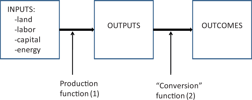
Production function of local public goods.
The local public sector produces “outputs.” Outputs represent the transformation of inputs (labor, capital, energy, land, etc.) through the production function and represent the efforts put forth by public agencies. Outputs range from million gallons of water treated per day to number of police patrols, to acres of parks provided, to lane miles of roads provided, to teacher–student contact hours.
Public sector “inputs” are nearly the same as in traditional production analyses: land, labor, capital, materials, and energy. These inputs are what show up in local government budgets. Aggregate expenditures on police, for example, represent labor costs for police officers, capital costs for stations, jails and patrol cars, fuel costs, and materials costs. The observed expenditures on police represent the number of input units (labor, capital, and fuel) multiplied by the cost per input unit (hourly wage, operating cost per square foot of building, etc.). In the production of “education,” inputs would be labor; school buildings; fuel for school busses, and so on, while for “water quality,” inputs would be labor of workers and capital such as pipes and treatment facilities.
Traditional “production function” analysis in economics maps the relationship between “inputs” and “outputs,” indicating how different inputs can be combined to produce a given level of output. This relationship is shown as “production function (1)” in Figure 2 above. The literature on measuring and modeling the production function is quite advanced (Kumbhakar and Tsionas 2011). For example, embedded in this production function can be economies of scale, economies of scope, network economies, economies of density, elasticity of substitution between inputs, factor input demands, and the elasticity of output with respect to factor input prices. All of these have been studied for private firms and industries, but few have been studied for local government service outputs. The lack of specific cost data and the conceptual difficulty between “outputs” and “outcomes” have hindered empirical work in this area.
Within production analysis, there is no analog for a process translating “outputs” into “outcomes” as shown in Figure 2. Here, a more generic term—the conversion function is used for lack of a commonly accepted alternative. The term conversion function is borrowed from the philosopher and economist Amartya Sen’s (1992) capability approach to utility. He describes differences among individuals in “converting” resources (such as income) into functionings and capabilities. By analogy, communities will differ in how they convert the outputs of local public services into LOS outcomes that voters care about. This conversion function for local public services could include environmental cost variables, congestion effects, and economies/diseconomies of density. However, the most significant component mediating how outputs translate into outcomes is likely the socioeconomic and demographic characteristics of the population itself. Unlike in standard analysis of market goods where demographic considerations are only found on the demand side, here they enter into the supply side of public goods through the conversion function. Beginning with the early work of Bradford, Malt, and Oates (1969), and continuing throughout the literature (Schwab and Oates 1991; Schwartz 1997), research on local public goods has recognized that the characteristics of the service population enter into the supply side. This has posed some empirical and theoretical difficulties for resesarch in this area. In the reduced form estimation stategy commonly employed, how should a researcher interpret coefficients on demographic variables if these variables represent both supply and demand factors?
Production and Conversion Functions in Detail
Beginning with the production function, this section will explain economies of scale, economies of scope, network economies, economies of density, and the elasticity of substitution between inputs as they relate to local public goods. Economies (diseconomies) of scale arise in those regions of production technology where average costs are greater than (less than) marginal costs or equivalently where the marginal cost of producing an additional unit of output decreases (increases) with the volume of the output. Alternatively, and perhaps more intuitively, economies (diseconomies) of scale occur where a 1 percent increase in inputs leads to more than (less than) a 1 percent increase in outputs. Within local public goods, there is strong and consistent evidence that most capital-intensive, utility-like public services (such as water supply, wastewater, solid waste, etc.) exhibit economies of scale (Callan and Thomas 2001; Duncombe and Yinger 1993; Hopkins, Xu, and Knapp 2004; Ladd 1998; Torres and Paul 2006). However, the literature on economies of scale in labor-intensive public services such as education and public safety remains ambiguous and lacking consensus (Gorman and Ruggiero 2008; Andrews, Duncombe, and Yinger 2002; Edwards and Huddleston 2010).
Economies of scope are less commonly estimated for public goods. Economies of scope exist when producing more than one product can reduce the production costs of each product, so that a multiproduct firm may be more efficient than a single-product firm. Shared inputs, bulk purchasing of common inputs, sharing of administrative and personnel services, and so on, may give rise to economies of scope. For local public services, this could imply that a general-purpose government providing a range of services may produce each service at lower per unit costs than if each service was provided by a separate level of government or private contractor. For example, there can be shared capital inputs between the parks department and the streets department, and workers and equipment can be moved from function to function based on seasonal variations. Common administrative services in terms of budgeting, payroll, and human resources may also provide cost savings. Callan and Thomas (2001) find significant economies of scope for cities which offer both solid waste and recycling services because of a significant overlap in shared inputs. Torres and Paul (2006) find economies of scope in municipal water supply services, which partially explains forces driving consolidation. Mays et al. (2009) find economies of scope in public health systems. Whether such economies of scope extend generally to local general-purpose governments is an open and understudied question.
Network economies generally refer to networked infrastructure systems (such as water supply, wastewater, utilities, and roads) where the relevant concept is not just volume of output, but its spatial distribution, connectivity, and density. The value of each connecting pipe or intersection is increasing in how many other pipes or intersections it is connected to. In practice, network economies as measured by customer density, length of network, number of nodes relative to network distance, and spatial extent of service area, are all likely to have significant influences on the cost structure providing public services (Torres and Paul 2006).
The area of local production of public goods which has generated some controversy in the planning literature is the concept of “economies of density.” By definition, economies (diseconomies) of density in production occur when, all else being equal, the cost per unit of a public service decreases (increases) with population or housing unit density. The literature on this question is not settled, as many methodological and data differences persist. Conceptually, the empirical problem in identifying economies of density is twofold. First, as above, empirical work is forced to utilize only expenditure data instead of cost data. The three major studies addressing this question at the level of overall local government services (Holcombe and Williams 2008; Carruthers and Ulfarsson 2008; Ladd 1992) use expenditure data. Second, as below, density can also be thought of as a variable that should enter into the “conversion” function. When a variable occurs twice in a theoretical model, but can only enter an empirical model once, there is no clear way to interpret the marginal interpretation of the variable’s coefficient.
Many capital-intensive utility-type environmental services (water supply, sewerage, and solid waste) have been shown to exhibit economies of density (Walter et al. 2009; Speir and Stephenson 2002). However, research on economies of density for labor-intensive public services (education, social services, and public safety) which comprise the largest share of local expenditures is limited and inconclusive. Ladd’s (1992) pioneering study of densities and expenditures only breaks out public safety expenditures and finds that public safety expenditures are increasing in density above a density of 250 persons per square mile. For comparison purposes, the US Census Bureau only classifies areas as “urban” with a minimum density of 500 persons per square mile (Paulsen 2012a). Carruthers and Ulfarsson (2008) break out expenditures in many public service categories, including education and police services, and include a more precise measure of density as persons per developed land area, rather than the entire area of the county as in Ladd (1992). Unlike Ladd, however, their model does not contain different categories of densities, thus unable to confirm or reject Ladd’s “U-shaped” evidence that expenditures are at first decreasing and then increasing with density. Carruthers and Ulfarsson (2008) find that overall local government spending is negatively related to density; that is, controlling for other demand and cost variables, increases in density are expected to reduce overall direct local government expenditures. Their estimated elasticity (at sample means) for density is −0.0136, indicating that as density increases by 1 percent, it is expected that expenditures will decrease 0.0136 percent. Although this might seem a small elasticity, given total local government direct expenditures of US$1.6 trillion, even small decreases in expenditures represent tens of billions of dollars. Carruthers and Ulfarsson also find a negative impact of density on spending on education, parks/recreation, and roads. Police expenditures are also negatively related to density, but significant only at the 10 percent level. Housing and community development expenditures are positively related to density, which is more likely related to demand rather than costs. They find no statistically significant relationship between density and expenditures for fire protection, libraries, sewerage, and solid waste.
There has not been much empirical work estimating the elasticity of substitution between inputs within the public sector, although this should be reasonably straightforward to do. The main reason for the lack of empirical research is that it is difficult to acquire consistent data across multiple cities measuring both input prices and input quantities. Such research would be helpful to the fiscal analysis of land development decisions if it indicates the degree to which there is sufficient flexibility within the local public sector to combine different inputs to produce outputs.
Moving from the production function to the “conversion” function, the relationships between outputs and outcomes have been more difficult to model or address in empirical work. Some differences across places in translating outputs into outcomes arise directly from the physical environmental factors such as climate or topography. To provide one lane mile of drivable roadway likely costs more in climates with frequent snowfall or mudslides or in steeply sloped areas. These differences are rarely accounted for in empirical work on local public spending. However, in this section, focus will be on what are likely the two most significant components of the “conversion” function—congestion effects and the socioeconomic/demographic characteristics of service populations.
Most local public goods are congestible, at least some of the time. Congestion occurs when service demands at a particular time exceed service capacity. Congestion shows up in the “conversion function” because congestion can alter the relationship between outputs and outcomes. The LOS experienced by residents and voters may be significantly impacted by congestion. As a result of congestion effects, there may not be a direct or consistent relationship between local expenditures and actual outcomes. In the same sense, one way that local officials can mitigate the direct fiscal effects of any particular land development is to let public goods get congested (decreased service level) without an increase in expenditure to restore service levels (Heikkila 1997; Heikkila and Craig 1991; Ladd 1994).
Conversion of local public goods outputs to LOS outcomes is shaped by the socioeconomic and demographic characteristics of the population itself. The literature describing these relationships has been called the community composition literature (Schwartz 1993, 1997; Schwab and Oates 1991). This literature raises both conceptual and empirical problems for researchers, as well as ethical issues for local planning.
One conceptual problem in research in this area has been “peer group effects” and “neighborhood effects” (Nechyba 2006; Calabrese et al. 2006; Hanushek et al. 2001; Hoxby 2000; Brueckner and Lee 1989). Peer-group and neighborhood effects refer to the fact that a person’s public good outcome depends on the characteristics of her peers or neighbors. Even given the same exact teacher, one student’s learning outcome might depend on his classmates, and given the exact same level of police resources, a person’s experience of safety could vary by neighborhood. The education literature has long recognized peer-group effects as having a significant impact on student achievement and aggregate test scores (Rivkin 2001). Much of the literature on local police expenditures has recognized neighborhood effects on crime and public safety (Sampson, Morenoff, and Gannon-Rowley 2002). Peer-group and neighborhood effects are not, of course, limited to education and public safety, but these two areas represent the most established lines of research.
The empirical problem in this research is, as above, that demographic variables can be interpreted both as demand characteristics and as “cost” characteristics in the conversion function. In practice, most studies estimate reduced-form regressions of expenditures on demographic variables along with policy, density, economic, and other variables as controls.
This extended tour through the production and conversion functions in local expenditures raises at least two direct implications for local fiscal analysis. First, as a practical matter, the processes involved in local public expenditure and LOS outcomes are more complex than can usually be represented in fiscal impact analyses. High-quality marginal-cost “case study” fiscal analysis techniques, where trained analysts or consultants interview department heads and examine local production structures and infrastructure capacity can possibly address most of the issues raised here in terms of the production function and congestion effects. However, these studies are generally expensive and perhaps beyond the capacity of many local governments or planners.
Second, the discussion of demographic characteristics in the “conversion” function, peer-group and neighborhood effects raise some complicated ethical issues regarding the use of fiscal analyses in local land use decision making. Most fiscal or land use analyses do not address the projected demographic characteristics of residents likely to move into the jurisdiction with a proposed land development. Even though the theoretical and empirical economic literature points to these demographic effects on outcomes, it is not at all clear that local planners or officials could or should consider these in decision making. Local planners and local officials know that to do so explicitly could potentially expose them to potential litigation for possible violation of civil rights or fair housing statutes. The only possible exception would be in regard to age-restricted developments for seniors. As both a practical and a legal strategy, local fiscal analyses only proxy these demographic characteristics indirectly through consideration of housing unit characteristics (number of bedrooms, average household size, density, etc.) and applying nationally or regionally derived “demographic multipliers.”
But the ethical issues become more complicated and controversial when examined in the light of the concept of “fiscally motivated exclusionary zoning” (Bogart 1993; Ihlanfeldt 2004; Schmidt and Paulsen 2009). It is likely the case that when local communities zone out or significantly restrict certain residential land uses (primarily higher-density, multifamily housing, and/or rental and/or affordable housing), some perceived “fiscal” concerns contribute to the decision to exclude. Regardless of the particular fiscal analysis technique used, lower-priced housing that is affordable for low- and moderate-income households will always show a “negative” fiscal impact or that such land use does not “pay its own way” because projected service demands exceed likely revenues attributable to the development. In many of the “standard” reference texts which planners use to learn fiscal impact methods (see, most recently, Bise 2011) something like the “fiscal hierarchy” of land uses is presented, with office parks on top as offering (in general) the “best” fiscal impact and mobile homes are on the bottom as offering (in general) the “worst” fiscal impacts. In the “hierarchy,” most rental housing (except one-bedroom units and condos) is below the municipal “break even” line because expected expenditures exceed expected revenues. It is important here to point out that the original presentation of the hierarchy in Burchell and Listokin (1978) strongly cautions readers that the hierarchy is a generalization, that local impacts could vary substantially due to a wide range of state and local structures, and that fiscal considerations alone should not guide land use decisions. Pointing out that some communities might use fiscal analyses as a (partial) justification for exclusionary zoning is not a critique of the method itself or the general use of fiscal impact techniques.
Understanding the “conversion function” and the concepts of peer group and neighborhood effects, however, adds a complication to the ethics of using fiscal criteria to make land use decisions. Voters who control both the local fisc and the local zoning decisions undoubtedly have certain assumptions about “peer-group” effects in local schools and “neighborhood effects” in terms of public safety. Therefore, “fiscally motivated exclusionary zoning” may not just be about the direct, measurable “fiscal loss” resulting from an apartment development, but may reflect existing residents’ beliefs that rental households’ lower socioeconomic status might negatively impact service quality (Schmidt and Paulsen 2009; Levine 1999, 2006; Paulsen 2006).
Land Development
This review began with an extended discussion of the determination of local public expenditures in “equilibrium”—before a land development. This tour through the expenditure determination process was designed to explicate all of the structures and processes of local public goods which are likely to mediate the impact of any land development on changes in local fiscal conditions. This conceptual model demonstrated the complexity of local public goods. In this section, the likely effects of a land development are traced through the system. Referring again to Figure 1, “direct” fiscal impacts are the shaded area in the center of the figure that deals with direct changes in revenues and direct changes in expenditures resulting from and attributable to the particular land development. These direct fiscal impacts have traditionally been the domain of fiscal impact analyses. However, as the discussion will make clear, direct fiscal impacts are likely only a small subset of the range of changes in local expenditures and revenues likely to result from land development.
In order to trace the effects of land developments through the local expenditure and revenue systems, two prototype developments are used as illustrations. “Development 1” is a large residential subdivision and “Development 2” is a mixed office and retail development.
Looking first at the demand for public services from Development 1, the new residents who occupy the newly constructed housing constitute new service demanding units for all areas of local expenditure. First, assume that new residents have exactly the same demand characteristics (e.g., tastes and income) of existing residents, an assumption to be relaxed later. These new residents need to be provided with education, public safety, and social services, roads, water supply, sewers, and the like. Apart from the cost and production function issues discussed below, translation of additional demand units into actual expenditures depends on whether slack capacity in service infrastructure is available and whether or not the local government responds to growth by allowing services to be congested or service quality to degrade. These new residents can directly impact expenditures in atleast one of the following four ways. First, to the extent that there is slack capacity within existing infrastructure systems, the new residents may be able to consume public services without necessarily increasing expenditures by a proportional amount. Second, conversely, to the extent that existing infrastructure systems are already at or near capacity, new residents may trigger large expenditures for increased/new infrastructure systems, which could result in an expenditure impact more than proportional to the population. Third, new residents could congest the public services (or degrade the LOS) if the local government is slow to respond with increased expenditures or if the local government does not increase expenditures proportionally (Heikkila 1997; Ladd 1994). Fourth, new residents could be accommodated with an exactly proportional increase in public expenditures, such that aggregate real per capita expenditures remain constant.
Even assuming the socioeconomic demand characteristics of new residents are exactly the same as existing residents, and assuming constant returns to scale in the public goods production technology (both strong and unlikely assumptions), new residents’ public service demands still yield ambiguous predictions in terms of changes in expenditures. A 1 percent increase in the population of the city can manifest in expenditures increasing:
by less than 1 percent (either due to slack capacity or due to degraded service levels/increased congestability),
by exactly 1 percent (maintenance of exact per capita expenditure levels), or
by more than 1 percent (due to capacity threshold effects).
There is no clear a priori way of determining whether expenditures will actually increase proportional to an increase in demand units. However, if the assumption that future residents have the same demand characteristics as existing residents is dropped, projections become even more difficult.
Now considering Development 2 (office and retail development), this land development will also see an increase in the number of service demanding units, here seen as employees, customers, and square feet of leasable space. Directly, the new employees will generate additional demand units for water and wastewater services, public safety, and will produce additional trips on local roadways. The new development will also produce customers or visitors, who will demand services such as roads, transportation, parking, public safety, and so on. Again, as above, how these additional demand units can be accommodated depends on the capacity of local infrastructure and whether they are accommodated through allowing congestion or a decrease in service levels.
Turning from demand characteristics to the production function of local public services, land development is likely to influence future expenditure patterns through altering the production function of public goods. In terms of production, many public services are likely to have different regions of the production technology where there are increasing, constant, and decreasing returns to scale (or scope, or density). Without a representation of the underlying production function, it is difficult to predict whether additional workers or new residents might move the city along its production function into an area of increasing or decreasing returns.
In terms of environmental cost variables, if the new development is less dense than existing development, or has more cul-de-sacs, or is located further away from the police and fire stations, for example, it may affect the costs of service delivery. In order to maintain a given LOS, expenditures may need to be increased more than proportionally. To the extent that the socioeconomic and demographic characteristics of (new) residents plays a significant role not only as a “demand” factor but as a “supply” factor mapping outputs to outcomes, land development which alters the existing socioeconomic composition of the community will also impact public services.
Property development or land use change alters the property tax base because new property value is added to the tax rolls. If the property tax levy (the amount raised by property taxes = property tax base multiplied by tax rate) is fixed, increased property values would lead to decreased property tax rates. Likewise, if property tax rates remain fixed, increases in property values would lead to increases in the tax levy. The dynamic impacts of new property value on the tax levy and tax rates will depend crucially on the state laws governing property tax administration and tax/expenditure limitations. In those jurisdictions with local income taxes, increases in residents would be associated with increased income tax collection. New residents would also pay user fees for those services financed with user fees. An increase in employees may be associated with increases in wage tax collections in jurisdictions with wage taxes. The retail component of Development 2 would also be associated with increased sales tax revenues in jurisdictions with in situ sales taxes.
In practice, projecting the likely direct own-source revenue changes resulting from a land development is reasonably simple and straightforward. However, projecting changes in outside-source revenues as a result of these land developments requires some understanding of the formulas used by the state to distribute educational and other local government aid. Based on some assumption of schoolchildren generating ratios, an analyst could project the likely increase in state aid to local schools as a result of the land development, particularly in those states where funding allocations follow a “foundation” model. However, in those states that use an “equalization” model, allocation formulas may include considerations of tax base, tax effort, and/or poverty rates. To the extent that the land development under analysis alters any of the variables in the state’s equalization formula, it may alter the outside-source revenue structure (Huddleston 2009). Changes in outside-source revenues attributable to the land development should still be considered “direct” fiscal impacts of the development, although such effects are rarely included in local fiscal analyses.
Indirect Fiscal Impacts
Returning again to the conceptual model presented in Figure 1, the previous section discussed direct changes in expenditures and revenues likely to result from a particular land development. These “direct” fiscal impacts are what are usually measured or estimated in fiscal impact analyses. All analysis, of course, necessitates assumptions, limitations, simplifications, and exclusions in order to be tractable, implementable, doable, and coherent or meaningful for public officials and citizens. All fiscal impact analyses make some assumptions and simplifications about the process of local public expenditure determination, as discussed above. Fiscal impact analyses also limit themselves to only direct fiscal impacts because direct impacts are more straightforward to explain and to avoid the problem of “double-counting.” The restricted domain of fiscal analyses to only direct impacts and the advantages and disadvantages of such restrictions have been recognized since the earliest days of the techniques (Burchell and Listokin 1978). However, whether such a limitation represents a prudent or necessary simplification continues to be a matter for evaluation and debate.
Consider again the concept or heuristic of “equilibrium.” When a system such as the local land use–public finance system experiences a “shock” (in this case, a land development), all elements of the system will adjust and respond to some new equilibrium. Adjustments and responses include not only “direct” changes (what are sometimes called first-round effects) but also what regional economic models would call “indirect” and “induced” effects (“second-round” and “third-round” effects) as prices, rents, incomes, and households all adapt in response to direct effects. The difference between the initial equilibrium and the new equilibrium is the net “impact” of the shock. In the local land use and public finance sector, these indirect and induced effects of any land development could include changes in prices and land values, capitalization of service/tax changes into land prices, spending by new residents, competition between businesses, and so on. While it may not be either fair, appropriate, or necessary to expect that local fiscal analyses must consider or model all of these indirect effects, the magnitude of these indirect effects still need to be considered. If indirect effects are larger in magnitude than the direct effects predicted in fiscal analyses, then land use and public expenditure decisions based on these fiscal analyses could possibly be considered “inaccurate” or “misleading.” While it is understandable from an accounting or legal perspective to avoid “double-counting” and only attribute to each land development its “direct” fiscal impact, in reality the full fiscal effects of any land development are likely to be larger than simply direct effects.
Limiting fiscal impact analyses only to “direct” impacts also manifests itself in what can be called the “attribution problem” in linking land uses to expenditures. Within the accounting framework used in most fiscal impact analyses, expenditure categories are allocated or attributed to particular land uses. Many services such as water supply or local roads or police expenditures need to be apportioned to commercial, industrial, agricultural, institutional, and residential land uses. Edwards and Huddleston (2010) review the methods used to attribute expenditures to land uses under the term allocation rule percentage. However, some expenditure categories are attributed to only one land use category by definition or assumption. Most notably, all public education expenditures are attributed only to residential land uses. Within a “direct” impact framework, this makes sense: only housing units generate schoolchildren. Hence, the need within fiscal analysis for current information on schoolchildren-generating ratios as important components in demographic multipliers (Burchell, Listokin, and Dolphin 2006). Office parks and retail facilities do not directly generate any schoolchildren and hence no educational expenditures are attributed to these land use categories. As a result, nonresidential land uses almost always show either a positive fiscal impact or a less-negative fiscal impact as compared to residential development. But this is by assumption in attributing only direct expenditures to particular land uses.
In this section, two of the features listed as “indirect” fiscal impacts in Figure 1 are explored, the likely indirect effects of changes in the local real estate market and the “multiplier” effect of changes in local employment or population. Because land development occurs within the local real estate context, one development is likely to impact other land values within a city. Changes in the property value or real estate market conditions on other properties within a city would constitute an indirect fiscal impact of the land development in question. Both the residential and the nonresidential development scenarios used here as illustrations could impact the property values of other properties within the city. For the example of Development 1, it is possible that additional new housing units could affect property values of existing housing units. Because homebuyers now have more units from which to choose, an oversupply could potentially depress price appreciation of existing housing. Conversely, the new housing—depending on its price and location—could increase the value of some existing homes. If there is a fixed amount of land available for retail development within the city, these additional housing units in the market area of existing retail could increase the property value of retail facilities. To the extent that increased or decreased property values lead either to increased or reduced property tax revenues or rates, these constitute indirect fiscal impacts of the land development.
A similar analysis can apply to Development 2, the nonresidential development illustrated here. The absorption of a significant amount of retail and/or office development within a city might depress the values of existing retail and office properties, as newer developments could lead to lower rents for existing properties. New retail development could draw business away from existing retail, depressing property values of existing retail centers. Even though the direct fiscal impacts of a retail or office development appear positive, the net result may not be as positive when declines in property values of existing properties are considered. It is also possible to imagine that large-scale retail and/or office developments could create positive spillover effects and increase the value of residential properties in the community, as employment or shopping opportunities are capitalized into residential land values. In such a case, the “direct” estimate of fiscal impacts from a retail or office development would underestimate the total fiscal effect.
The second area where land development is likely to lead to indirect fiscal impacts, shown on the bottom of Figure 1, is through the “multiplier” effect of changes in local employment or population. When new office or retail facilities are developed, this creates jobs and potentially increases local employment. These new employees need places to live, possibly inducing housing construction and development. This induced residential development has its own “direct” fiscal impact, but it also constitutes an “indirect” fiscal impact of the office or retail development. Recall from above that in the “fiscal hierarchy,” office and retail development are generally thought to result in fiscal surpluses for a community, but this is largely due to the attribution of all education expenditures to residential and none to office or retail. It should be clear, however, that the workers to be employed will live in houses and send their children to the public schools. If an office or industrial or retail development draws new residents into a community, these residents’ public expenditure demands are an indirect fiscal impact of the development. Likewise, new housing units and residents will generate demand for additional retail land development and service-based land uses such as medical offices, hospitals, churches, and so on.
In all of these cases presented, there is no a priori way to know whether the magnitude or direction of indirect effects would overwhelm the direct effects predicted in fiscal impact analyses. If indirect effects are significant enough, their exclusion from fiscal impact analyses could potentially influence local land use decision making toward potentially incorrect conclusions and policies. Consider three reasonably common local land use issues where the absence of indirect effects in fiscal analysis might create inefficient or inequitable policy outcomes. First, age-restricted developments for seniors (over age fifty-five) are one of the fastest growing segments of the housing market, reflecting not just an aging population but local governments’ beliefs that age-restricted developments contribute fiscal surpluses. Many local governments seem more willing to approve age-restricted developments than housing for families. When direct fiscal impact analyses are conducted, senior housing generates a fiscal surplus because no school-age children are generated. But such a view tends to ignore the idea that housing units themselves go through cycles of demographic evolution as households move through various stages in the life cycle. These senior households could have themselves had school-aged children at one time. Households who move into age-restricted housing (or smaller town houses or condos) are likely to move out of their existing single-family detached houses. Families with schoolchildren then buy the existing single-family detached house, thereby “generating” new schoolchildren “demand units” and an increase in educational expenditures and/or a congestion of service quality. Thus, the potential forecasted “fiscal surplus” of senior housing would be reduced.
Second, consider that a community seeks a large “big-box” retail center to add to its tax base, because of the belief that such centers generate fiscal surpluses. However, as the general critique of big-box retail holds, smaller local retail businesses are likely to experience declining business. In a recent study, Haltiwanger, Jarmin, and Krizan (2010) find substantial negative impacts of big-box entry on existing smaller local stores. If existing local businesses see declines in sales and employment, there is a corresponding decline in property values (and therefore property taxes paid) and a decline in possible sales or wage tax receipts. Alternatively, if the big-box retail center increases overall employment in the city, this might induce more residents to move to the community, generating additional expenditure demand. As such, any “fiscal surplus” from a retail development may be reduced or eliminated.
Third, the results of direct fiscal analysis might suggest to a community rejection of higher-density town houses or apartments with multiple bedrooms per unit and to instead prefer more expensive single-family housing or one-bedroom rental units. However, one result of such decisions may be to limit the availability of affordable “workforce” housing. If businesses in the community are unable to attract workers because of a lack of workforce housing, then these employers may eventually leave the city or region for other places, reducing tax receipts and income within the community.
Discussion and Implications
Local land use planners and decision makers—and indeed local voters—have taken great interest in trying to understand the likely fiscal effects of land development decisions. Understandably so: local taxes are a significant burden on most households, local public services are critical to most households’ quality of life, and a person’s home is usually their most valuable asset. The purpose of this review was to provide a conceptual framework for thinking about the likely impacts of land development on local expenditures and revenues and the extent to which local fiscal analyses adequately capture these impacts. The results of this review could no doubt be construed as being unhelpful or very impractical for local land use and fiscal planning for two reasons. First, if academic public finance economists cannot identify the equilibrium properties of conjoined local housing and public finance models, how are local practitioners expected to predict or know the likely total impacts (direct and indirect)? If academic models have difficulty characterizing the complexity involved in the system, what possible framework for decision making should local planners rely on? Second, the discussion in this review was termed, perhaps somewhat jokingly, an “impossibility theorem” by a prominent scholar when first presented. Does the argument that there is no way a priori to predict the direction and magnitude of the relationships between land development and municipal finance really mean that the practice of fiscal impact analysis should be abandoned? No. But this review does call for reform, caution, more careful practice and additional research, but not abandonment. The next section discusses the implications for practice and the final section proposes some implications for future research.
Implications for Practice
There are two main categories of implications from this review for local fiscal and land use planning: “understand more fully” and “use more cautiously.” The first implication is that local planners, fiscal analysts, citizens, and decision makers should understand more fully how the various fiscal impact methods utilized actually work and what useful information these methods can and cannot produce. Most fiscal impact analyses, even when jurisdiction-specific case study methods are used, are conducted within an “accounting” framework rather than what could be called an econometric framework. Fiscal analyses all include some means of allocating or assigning various expenditure categories or budget components to various land use categories. In order to make the framework work, all expenditures are assigned to land use categories. This is the static accounting sense where everything adds up and all expenditures are explained by the land uses within the community. The accounting framework does provide an apparent conceptual validity to estimates because everything is accounted for in ways decision makers can understand. But the assumptions and techniques used to assign expenditures to particular land uses are not based on any actual research (Edwards and Huddleston 2010). In addition, as discussed above, the accounting framework assigns all educational expenditures to residential uses. Because educational expenditures are the largest component of local expenditures, this assumption can drive the results of analyses.
Accounting frameworks are useful for avoiding “double counting.” One critique of the discussion above of second-round and indirect effects is that such analyses could lead to double counting if expenditure changes are attributed both to the residential and to the commercial development. Especially in cases where fiscal impact analyses are used to inform impact fees or developer agreements, avoiding “double counting” is both a legal and a financial necessity. However, accounting-type analyses are often inadequate methods for predicting changes in dynamic systems. If all expenditures are fully apportioned to all of the land uses within a community, then it would not be possible for expenditure changes to arise from any source outside of land use change. But this is clearly not the case, as there are multiple reasons why expenditures might change in a community without any changes in land use.
Planners and local decision makers need to understand the relationships between land development and public finance in order to evaluate fiscal methods and analyses. One implication of the literature reviewed here is that planners and decision makers need to understand all of the assumptions involved in fiscal impact analyses and how those assumptions can often drive the results of the analysis. The output of a fiscal analysis may appear to offer decision makers some knowledge or certainty about likely fiscal impacts of a land development, but this certainty may not actually be warranted by the methods themselves.
Second, planners and local decision makers need to interpret and use the results of fiscal analyses more carefully. This certainly means to state all assumptions clearly and explicitly, as in fact, thoughtful practitioners do and as standard references suggest (Bise 2011). Discussion of the assumptions and limitations of fiscal impact analyses can be used to educate and inform voters about the range of likely impacts of land development, even those possible indirect effects not included in the analysis. More careful use of analysis tools also involves clearly customizing the analysis to the specific local and regional context and not solely relying on “off-the-shelf” models or tools. In this regard, again, the survey results in Edwards and Huddleston (2010) that case study techniques are now more commonly used that per capita multiplier techniques is encouraging.
However, recommendations for more careful and nuanced presentation of fiscal impact analyses are made with the awareness that local government budgets are continuously under pressure and local officials face tremendous difficulties responding to voters’ concerns, regional competition, and state fiscal and land use institutional structures. As decision makers try to make land use and fiscal decisions with limited resources and limited information, there can possibly be pressure for the fiscal impact analysis to be used as a decision tool rather than as only one of multiple impact analysis and planning tools. Although analysts and planners who prepare fiscal impact studies understand the limitations and assumptions inherent in the analysis, officials or voters can often exert pressure on analysts to “just give me a number!” (Moore et al. 2004).
Planners also should be careful to understand the subtle ways in which fiscal analyses and fiscal concerns can possibly influence or contribute to exclusionary zoning. As currently structured, fiscal impact analyses will not show any direct fiscal surplus to communities for zoning to allow higher-density multifamily rental housing affordable to low- and moderate-income families. This can pose some ethical difficulties for local planners and decision makers and should encourage planners to develop creative strategies, policies, and partnerships to encourage communities not to misuse fiscal criteria as a basis for exclusion.
Implications for Research
This review has identified a number of areas in research where additional research could improve understanding and practice. In this section, implications for research focus on two areas, methodology and policy analysis. Methodological research here refers to research designed to produce improved tools, data, models, or methods for use by practitioners. Six particular areas of future research emerge from this review. First, there is clearly the need to produce and acquire more data and research on the cost structure of local public goods. This review began by pointing out the absence of high-quality cost data, instead forcing the use of expenditure data in analysis. Research to produce high-quality cost data could proceed along the lines of empirical production analysis, specifically using methodologies designed to estimate cost functions (Pope and Just 1998). Alternatively, case study approaches could be used to sample a limited number of cities and conduct detailed interviews and examination of historical budget documents and department reports to construct detailed records of the relationship between costs and expenditure levels.
Second, the review identified only a limited number of empirical studies that have directly and jointly estimated something like the production and conversion functions. Additional work in this area could provide more insights into local public goods production. Many of the existing empirical studies estimate these relationships in a cross-section framework, but as more historically consistent data becomes available, change analysis and fixed effects panel estimation strategies could be employed. Third, this review identified that the literature on the effect of density on public expenditures has not reached a consensus. Shaping land uses toward greater urban density has been one of the central emphases in much of the planning and “smart growth” literature. However, the existing literature on density as it relates to public expenditures is confusing. The “fiscal hierarchy” of land uses often suggests to communities that higher-density development is not fiscally advantageous, while the “smart growth is more fiscally efficient” literature (Speir and Stephenson 2002; Carruthers and Ulfarsson 2008) argues that more dense growth reduces expenditures. Here is clearly a case where more research could help provide empirical grounding to planning practice.
Fourth, there is a need for more empirical work on demographic multipliers and the demographic evolution of housing units, as described previously. Demographic multipliers play a significant role in impact analyses, particularly the average per capita methods. Estimates of multipliers are usually produced using cross-section data only for new housing units. More empirical work on this topic could use panel methods to estimate how household size and composition adapts to new housing unit construction in a jurisdiction and to estimate the indirect effects of new housing construction on the demographic composition of existing housing units. Research on the demographic evolution of housing units is needed to help place demographic multipliers in a longer time framework. Many fiscal impact analyses are limited to fifteen or twenty years, and understandably so because forecast error is magnified over time and fifty-year estimates would be highly unreliable. However, consider the demographic evolution of a typical new detached house. For the first twenty or so years of its lifetime, the housing unit could produce some number of schoolchildren who need to be educated in the public schools. Then, as the children maturate and the parents “age-in-place,” the same housing unit would be paying property taxes but not contributing schoolchildren expenditure need. As the owners age and retire, they might move to a one-bedroom town house, thereby opening up the detached house to a new young family with school-age children to acquire. Decisions about what types of housing units to produce in a community are sometimes based on these short-run fiscal impact analyses which utilize existing demographic multipliers. But such analyses would likely miss the fact that housing units are durable over multiple decades, and the demographics of future occupants may be substantially different than those predicted in shorter-term fiscal impact analyses. Over the first twenty years after its construction, a housing unit with four bedrooms may show a net “fiscal loss,” while over seventy-five years of its life the net fiscal impact may be neutral or positive.
Fifth, following the suggestion in Edwards and Huddleston (2010), additional research is needed to provide an empirical basis for allocating expenditures across land use classes. In their review of “allocation” practice, communities use land area percentages, number of parcels, parcel value, or even measures of parcel size such as street frontage to allocate expenditures. Many of these assumptions are intuitively justified, but are ad hoc without empirical foundations.
Sixth, there is a need for research to produce more robust econometric models of local public expenditures and land use change which can be made available to practitioners. As above, it is certainly not fair to expect overworked and underresourced local planners to produce sophisticated econometric models of the local public sector. Practitioners and analysts use the methods and tools which researchers produce. States that place a great emphasis on local fiscal impact analysis could fund development of customized, state-specific econometric impact models and make them available to communities through technical assistance. Alternatively, fiscal models could be added to existing models used to evaluate economic development policies or forecast local economic output.
The second broad category of research needs identified is in the area of policy analysis, where research is needed to examine the variation across places and policy regimes in the use of fiscal considerations in land use decision making and the relationships between land development and public finance outcomes. Much of the empirical work so far has either been detailed analysis in one state or region or national in scope. But states and regions vary significantly in the institutional structure governing land development and public finance. Research in this category could be used to reform state policy and legal–institutional structures governing land development.
Three specific research questions follow from this review. First, to what extent do communities rely on fiscal criteria in decision making over future land uses? Specifically, it is hypothesized that fiscal considerations are more likely to influence land use decisions in places with a greater dependence on own-source revenues. Higher dependence on own-source revenues, particularly the property tax, provides greater incentive to communities to engage in “fiscal zoning.” Second, and related, how do state equalization and municipal aid formulas impact the incentives of municipalities to “chase ratable” and engage in exclusionary zoning? The specific hypothesis here is that states with more equitable equalization schemes should see reduced municipal incentives to chase ratables and exclude rental housing. A related policy analysis hypothesis would examine the extent to which fiscal incentives could be used by a state to encourage communities to accept higher-density development and particularly rental housing for moderate-income families. One of the underlying arguments here has been the idea that some communities exclude affordable and/or higher-density housing because of fiscal concerns. If that is true, how can states design fiscal incentive schemes to mitigate fiscally motivated exclusionary zoning? The third specific area for research is to examine how the “renter effect” varies by state. All of the extant empirical work on the renter effect is either national in scope or state-specific. Research is needed to see whether the renter effect holds differentially across states and regions. Specifically, does the “renter effect” hold the same in states with “uniformity” provisions for property taxation and those allowing differential taxation? Does the “renter effect” differ between cities with at-large city council elections and those with districts? Do TELs reduce or mitigate the renter effect?
Conclusion
The purpose of this article was to provide a conceptual understanding of the fiscal effects that might be expected to result from land development within a community to serve as a basis for understanding, evaluation, and potential improvement of fiscal impact analyses. The underlying mechanisms by which local public expenditures are determined, produced, and experienced have a richness and complexity which can often be obscured or assumed away in fiscal impact analyses. Understanding and predicting the effects of land development on municipal revenues and expenditures begins with an understanding of public expenditure determination in the complex interaction between demand for public services and the production and conversion functions translating public inputs and outputs into LOS outcomes experienced by voters and residents. Tracing the effects of land development through this system requires assumptions about service demands, service production, and the effects of socioeconomic and demographic characteristics on both demand and costs. Those direct fiscal impacts that are measured in most fiscal impact analysis techniques are only a subset of the range of fiscal impacts that would likely be expected to result from land development within a community.
Footnotes
Acknowledgements
The research presented here was originally presented at a seminar (and later distributed as a Working Paper) sponsored by the Lincoln Institute of Land Policy. It was also presented at the Association of Collegiate Schools of Planning conference. At those seminars, I received helpful comments from Jeffrey Chapman, Tim Chapin, Randy Crane, Jacqueline Geoghegan, Greg Ingram, Zenia Kotval, Joe Marlow, Matthew Morrissey, Chris Nelson, Andy Reschovsky, and Amy Schwartz. I especially want to thank my research partners Mary Edwards and Samina Raja. I thank Jack Huddleson and Rosalind Greenstein for mentoring this project and reviewing multiple drafts. All remaining errors are my own and the opinions and ideas expressed in this article do not reflect the views of the Lincoln Institute, its funders, board or staff.
Declaration of Conflicting Interests
The author(s) declared no potential conflicts of interest with respect to the research, authorship, and/or publication of this article.
Funding
The author(s) disclosed receipt of the following financial support for the research, authorship, and/or publication of this article: Lincoln Institute of Land Policy.