Unions and Income Inequality

Abstract

In this research note it is shown that, by applying cointegration and causality techniques to U.S. state-level panel data, there is a negative long-run relationship between unionization and income inequality in the United States, and that causality is unidirectional from unionization to inequality.

Keywords

unions income inequality panel cointegration causality

During the past four decades, the United States, like many other nations, has experienced an increase in income inequality and a decline in union density. However, although a large body of research has examined the effects of unions on the U.S. wage distribution, only one study to date has explicitly examined the effects of unions on U.S. income distribution. Partridge, Rickman, and Levernier (1996) found, using data from 48 U.S. states for the period 1960 to 1990, that unionization has no statistically significant impact on income inequality.

Theoretically, unions can affect the distribution of income through several mechanisms, such as wage inequality, unemployment, and the wage share. As far as the mechanism of wage inequality is concerned, unions tend to reduce wage inequality within the union sector by pushing up the wages of low-skilled workers more than those of high-skilled workers, while they tend to increase wage inequality between unionized workers and nonunionized workers by raising the wages of their members relative to the wages of nonunionized workers (Checchi & García-Peñalosa, 2010).

As far as the effects of unions on employment are concerned, the traditional view is that an increase in union membership increases the bargaining power of unions, which enables unions to raise wages above the competitive market-clearing level. When unions fix wages at a level in excess of that at which all workers can be employed, some workers are unemployed. Higher unemployment, in turn, increases the proportion of people receiving unemployment benefits. Because income from unemployment benefits is typically less than income from work, an increase in unemployment increases the proportion of people with low incomes; this is generally associated with increased income inequality. The alternative view is that unions care about both wages and employment, and that in an imperfectly competitive labor market environment there is a scope for unions to increase wages at the expense of reductions in profits without adverse impacts on employment (Checchi & García-Peñalosa, 2010).

Although both wage inequality and unemployment increase income inequality, the effect of the wage share on income inequality is ambiguous. A higher wage share reduces the contribution of inequality of capital income to total income inequality but increases the contribution of wage inequality to total income inequality (Checchi & García-Peñalosa, 2010). Because the inequality of capital income is likely to exceed the inequality of wage income (Glyn, 2009), it is reasonable to assume that an increase in the labor share decreases income inequality.

As discussed in Bentolila and Saint-Paul (2003), unions can positively or negatively affect the labor share. If unions and firms bargain over both wages and employment, and workers are able to obtain a higher wage without suffering a decrease in employment, the labor share will increase. If unions and firms instead bargain only over wages, leaving firms free to determine employment unilaterally, higher union wages may combine with lower employment. In this case, an increase in union power can lead to a lower wage share.

Thus the net effect of unions on the distribution of income is theoretically unclear. However, it could also be that income inequality affects union density. Inequality-averse union members may perceive unions as unable to reduce wage inequality and to influence redistributive policy when inequality increases. If these individuals feel that their expectations regarding the efficacy of unions in reducing inequality have been disappointed, income inequality can lead to de-unionization (Checchi, Visser, & van de Werfhorst, 2010). Thus the direction of causality is also an open question, and this is one question the present study attempts to answer.

The objective of this research note is to examine the long-run relationship between unionization and income inequality in the United States using state-level panel data for the period 1964 to 2012. Specifically, the study makes the following contributions: First, I use panel cointegration methods to avoid spurious regressions in panel data. As discussed in more detail in the next section, panel cointegration estimators are robust under cointegration to a variety of estimation problems that often plague empirical work, including omitted variables and endogeneity (Coe, Helpman, & Hoffmaister, 2009). Moreover, panel cointegration methods can be implemented with shorter data spans than their time-series counterparts. Second, I use panel methods that explicitly account for potential cross-sectional dependence due to common shocks or spillovers among cross-sectional units at the same time. Failure to control for such unobserved common time-specific factors can lead to inconsistent estimates if these omitted factors are correlated with the explanatory variables and/or are nonstationary (Kapetanios, Pesaran, & Yamagata, 2011). And finally, I use a panel vector error correction model (VECM) to test the direction of causality.

The next section presents the basic empirical model, discusses some econometric issues, and lays out the empirical strategy. The third section presents the empirical results and the final section concludes with a summary of the main findings.

Model Specification and Empirical Strategy

Basic Model

The basic model takes the form

T O P D E C I L E_{i t} = a_{i} + β U N I O N_{i t} + ε_{i t},

where TOPDECILE_it is the income share of the top decile over time periods $t = 1, 2, \dots, T$ and states $i = 1, 2, \dots, N$ , and UNION_it is union density in state i in year t. I choose the top decile income share as my measure of income inequality because it is commonly used (see, for instance, Andrews, Jencks, & Leigh, 2011; Chintrakarn, Herzer, & Nunnenkamp, 2012; Frank, 2009; Piketty & Saez, 2006) and because the available income data do not permit accurate calculation of the Gini inequality index (Frank, 2009). The coefficient β represents the cross-state average of the state-specific effects of unionization on income inequality. It is estimated based on the mean group approach, which involves first estimating separate time-series regressions for each state and then averaging the individual state coefficients β_i (as described in Equation 3 below). Consequently, the β_i are allowed to be state specific and thus to vary across states. Finally, a_i represent the state-specific intercepts of the individual time-series regressions, thus capturing any state-specific omitted factors that are relatively stable over time.

The data on the top 10% income shares are drawn from the updated database of Frank (2009; available at http://www.shsu.edu/~eco_mwf/inequality.html), and the data on union density are from the Union Membership and Coverage Database constructed by Barry Hirsch and David Macpherson (available at http://www.unionstats.com/). Given that the longest period for which data on both variables are available for all 50 U.S. states and the District of Columbia is 1964 to 2012, the panel includes 2,499 observations on 51 cross-sectional units and 49 years.

I now discuss some econometric issues regarding the estimation of the long-run effect of unions on income inequality. These issues are grouped under four headings: (a) nonstationarity and cointegration, (b) omitted variables, (c) cross-sectional dependence, and (d) causality.

Nonstationarity and Cointegration

Whereas in all states there is a downward trend in union density since 1980 (or earlier), the income share data reveal a strong increase in inequality since the 1980s (or earlier) in all states, as shown in Figure 1. Such time series (that show no tendency to return to a constant mean) are said to be nonstationary.

Figure 1.

TOPDECILE_it (▬) and UNION_it (─) over the period 1964 to 2012.

Given that most economic time series are characterized by a stochastic rather than deterministic nonstationarity, it is reasonable to assume that the trends in TOPDECILE_it and UNION_it are also stochastic through the presence of a unit root, rather than deterministic through the presence of polynomial time trends. In particular, it is likely that the two variables have one unit root, as is typical for most economic time series. Such time series are said to be integrated of order one or I(1); an I(1) variable must be differenced one time to make it stationary or I(0).

If TOPDECILE_it and UNION_it are driven by separate I(1) trends, then any linear combination of these variables will also be I(1). In this case, there is no relationship between TOPDECILE_it and UNION_it, implying that Equation 1 is a spurious regression. As shown by Entorf (1997) and Kao (1999), the tendency for spuriously indicating a relationship may even be stronger in panel data regressions than in pure time-series regressions. When variables are nonstationary, standard regression output must therefore be treated with extreme caution because results are potentially spurious.

If, in contrast, TOPDECILE_it and UNION_it share a common stochastic trend (and no irrelevant nonstationary variables are included), then a linear combination of these variables will be I(0). In this case, TOPDECILE_it and UNION_it are said to be cointegrated. Cointegration implies the existence of a long-run relationship between two or more integrated series. Cointegration of TOPDECILE_it and UNION_it is thus the condition required for Regression 1 not to be spurious—a condition that must be tested.

Omitted Variables

A regression containing all the variables of a cointegrating relationship has a stationary error term, implying that no relevant integrated variables are omitted; any omitted nonstationary variable that is part of the cointegrating relationship would become part of the error term, thereby producing nonstationary residuals and thus leading to a failure to detect cointegration. If there is cointegration between a set of variables, then this stationary relationship also exists in extended variable space. In other words, the cointegration property is invariant to model extensions, which is in stark contrast to regression analysis where one new variable can alter the existing estimates dramatically (Juselius, 2006). Thus an important implication of finding cointegration is that no relevant nonstationary variables are omitted and that no additional variables are required to form a cointegrating relationship.

Of course, there are many factors that can affect income inequality and/or union density. Therefore, adding further nonstationary variables to the model may, on one hand, result in further cointegrating relationships (see, for instance, Brückner, Gerling, & Grüner, 2010). If, however, there is more than one cointegrating relationship, identifying restrictions are required to separate the cointegrating relationships. Otherwise, multicollinearity problems may arise. On the other hand, adding further nonstationary variables to the regression model may result in spurious associations. More specifically, if a nonstationary variable that is not cointegrated with the other variables is added to the cointegrating regression, the error term will no longer be stationary. As a result, the coefficient of the added variable will not converge to zero, as one would expect of an irrelevant variable in a standard regression.

Although these considerations justify a parsimonious model such as Equation 1 (if cointegrated), I nevertheless check the robustness of the results to the inclusion of additional variables, such as real state income per capita (INCOME_it), real state income per capita squared (INCOMESQ_it), and two measures of education: the proportion of the population with at least a high school degree (HIGHSCHOOL_it) and the proportion with at least a college degree (COLLEGE_it).

INCOME_it is intended to pick up the impact of the level of economic development on inequality. INCOMESQ_it is included to test whether there is an inverted-U relationship between income inequality and economic development, as proposed by Kuznets (1955), or whether the inequality-development relationship in the postwar United States is U-shaped, as found by Ram (1991) and Jacobsen and Giles (1998). As far as the education variables are concerned, several cross-national studies find a strong negative association between inequality and education, particularly secondary education (see, for instance, Nielsen, 1994; Nielsen & Alderson, 1995). The intuitive explanation, which is based on supply and demand for educated workers, is that increased availability of qualified personnel increases competition and produces a relative decline in the higher wages and salaries (Nielsen & Alderson, 1995). As a test of this explanation, I include HIGHSCHOOL_it and COLLEGE_it.

The income data are from the Regional Accounts Data of the Bureau of Economic Analysis (available at http://www.bea.gov/itable/iTable.cfm?ReqID=70&step=1#reqid=70&step=1&isuri=1) and are deflated using the consumer price index. The education data are from the updated database of Frank (2009). Because these data are available only up to 2010, I am forced to use the period 1964 to 2010 in the robustness checks.

Cross-Sectional Dependence

Another issue is the potential cross-sectional dependence of the data due to omitted common factors. Common factors may be a combination of “strong” factors representing national shocks, such as common business cycles, national financial crises, and macroeconomic policies at the federal level, and “weak” factors such as spatial spillovers between a limited number of states (Holly, Pesaran, & Yamagata, 2010). If both TOPDECILE_it and UNION_it share common factors f_t, such that $ε_{i t} = ρ_{i} f_{t} + ν_{i t}$ and $U N I O N_{i t} = c_{i} + γ_{i} f_{t} + υ_{i t}$ , estimating Equation 1 without accounting for f_t will produce biased estimates of β. If, in addition, some of the common factors are nonstationary, failure to account for them can lead to spurious regression results.

The standard approach to account for omitted common factors is to use demeaned data in place of the original data, which in pooled models is equivalent to the use of time dummies. The implicit assumption behind this approach is that the factor loadings of the common factors are homogeneous across the cross-sectional units, $ρ = ρ_{i}$ and $γ = γ_{i},$ and, consequently, that the impact of the common factors does not differ across the cross-sectional units.

An alternative approach is to use the common correlated effects (CCE) mean group estimator of Pesaran (2006). This estimator accounts for cross-sectional dependencies that potentially arise from multiple common factors and permits the individual responses to the common factors to differ across panel members. Another advantage is that the CCE estimator can be computed by ordinary least squares (OLS). The idea of the CCE estimator is to account for common factors by augmenting the estimating equation with cross-sectional averages of the dependent variable and the observed regressors as proxies for the unobserved factors. The cross-sectionally augmented regression of (1) for the ith cross-section is as follows:

\begin{array}{l} T O P D E C I L E_{i t} = a_{i} + β_{i} U N I O N_{i t} + \\ g_{1 i} \bar{T O P D E C I L E_{t}} + g_{2 i} \bar{U N I O N_{t}} + e_{i t}, \end{array}

where $\bar{T O P D E C I L E_{t}} = N^{- 1} \sum_{i}^{N} T O P D E C I L E_{i t}$ is the cross-sectional average of TOPDECILE_it and $\bar{U N I O N_{t}} = N^{- 1} \sum_{i}^{N} U N I O N_{i t}$ is the cross-sectional average of UNION_it.

The mean group procedure involves estimating separate regressions for each state and averaging the long-run coefficients. The mean group estimator and its standard error are calculated as follows:

\hat{β} = \bar{β} = \frac{\sum_{i = 1}^{N} {\hat{β}}_{i}}{N},

s e (\hat{β}) = \frac{σ ({\hat{β}}_{i})}{\sqrt{N}} = \sqrt{\sum_{i = 1}^{N} \frac{{({\hat{β}}_{i} - \bar{β})}^{2}}{(N - 1)}} / \sqrt{N} .

While Pesaran (2006) proves the consistency of his estimator under the assumption that both the variables and the (unobservable) common factors are stationary, Kapetanios et al. (2011) show that the CCE estimator is consistent even when the data follow a unit root process, provided that the series involved are cointegrated.

Causality

It is well known that even the standard OLS fixed effects estimator is a consistent estimator of the cointegrating relationship and can therefore be used to estimate the cointegrating coefficients, even if the regressors in the cointegration relationship are endogenous. The problem is that in the presence of endogeneity (or reverse causality) the OLS t ratio is not asymptotically standard normal and thus useless for inference.

A related issue is that, although the existence of cointegration implies long-run Granger causality in at least one direction (Granger, 1988), cointegration does not indicate the direction of long-run causality. The standard approach to test for long-run causality (or weak exogeneity) in cointegrated panels is a two-step procedure (see, for instance, Canning & Pedroni, 2008; Eberhardt & Teal, 2013; Herzer, Strulik, & Vollmer, 2012).

In the first step, the previously estimated long-run relationship is used to construct the error correction term $e c_{i t},$ defined here as

e c_{i t} = T O P D E C I L E_{i t} - ({\hat{a}}_{i} + \hat{β} U N I O N_{i t}) .

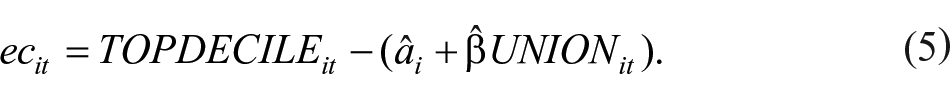
In the second step, the lagged error correction term is entered into a panel VECM, given here by

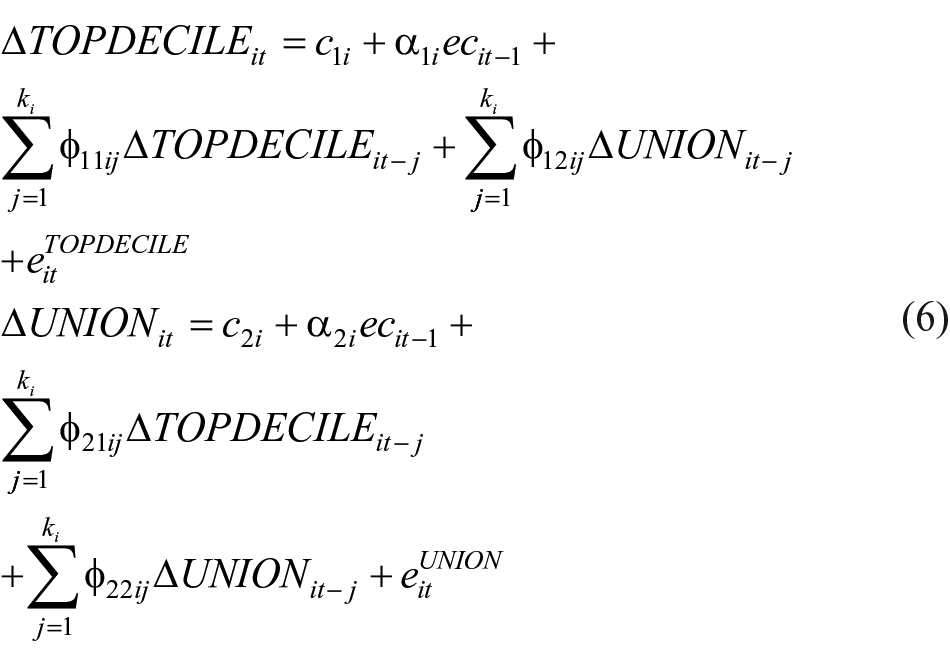
\begin{array}{l} Δ T O P D E C I L E_{i t} = c_{1 i} + α_{1 i} e c_{i t - 1} + \\ \sum_{j = 1}^{k_{i}} ϕ_{11 i j} Δ T O P D E C I L E_{i t - j} + \sum_{j = 1}^{k_{i}} ϕ_{12 i j} Δ U N I O N_{i t - j} \\ + e_{i t}^{T O P D E C I L E} \\ Δ U N I O N_{i t} = c_{2 i} + α_{2 i} e c_{i t - 1} + \\ \sum_{j = 1}^{k_{i}} ϕ_{21 i j} Δ T O P D E C I L E_{i t - j} \\ + \sum_{j = 1}^{k_{i}} ϕ_{22 i j} Δ U N I O N_{i t - j} + e_{i t}^{U N I O N} \end{array}

where k is the lag length (which is determined by the Schwarz criterion), $e c_{i t - 1}$ represents the deviation from the equilibrium, and the adjustment coefficients α₁ and α₂ capture how TOPDECILE_it and UNION_it respond to deviations from the equilibrium. The Granger Representation Theorem (Engle & Granger, 1987) implies that for a long-run equilibrium relationship to exist between TOPDECILE_it and UNION_it at least one of the adjustment coefficients must be nonzero.

If the adjustment coefficient in the ΔTOPDECILE_it equation is nonzero, $α_{1} \neq 0,$ then the null hypothesis of weak exogeneity is rejected for TOPDECILE_it. If the adjustment coefficient in the ΔUNION_it equation is nonzero, $α_{2} \neq 0,$ then the null hypothesis of weak exogeneity is rejected for UNION_it. Hall and Milne (1994) show that weak exogeneity in a cointegrated system is equivalent to the notion of long-run noncausality (see also Granger, 1988). Thus if (and only if) $α_{1} \neq 0,$ then UNION_it has a causal impact on TOPDECILE_it in the long run; if (and only if) $α_{2} \neq 0,$ then TOPDECILE_it has a long-run causal impact on UNION_it; if both α₁ and α₂ are nonzero, then long-run Granger causality runs in both directions (see also Eberhardt & Teal, 2013).

To account for cross-sectional dependence, I (again) compute the CCE mean group estimator. Accordingly, Equation 6 is augmented with cross-sectional averages of the dependent variables and the regressors, including $e c_{i t - 1} .$

Thus the empirical strategy involves three steps. First, the relevant variables are pretested for unit roots and cointegration. In the second step, the long-run relationship is estimated and the robustness to the inclusion of additional variables is examined. Finally, the question of causality is investigated.

Empirical Analysis

Panel Unit Root and Cointegration Tests

Given that so-called first-generation panel unit root tests, which assume cross-sectional independence can exhibit severe size distortions in the presence of cross-sectional dependence, I employ a second-generation panel unit root test to account for potential cross-sectional dependence. More specifically, I use the cross-sectionally augmented Dickey–Fuller test (ADF) panel unit root test proposed by Pesaran (2007). This test, which is based on an average of the individual (state specific) ADF t statistics, is designed to filter out the cross-sectional dependence by augmenting the individual ADF regressions with the cross-sectional averages of lagged levels and first differences of the individual series (as proxies for the unobserved common factors).

Table 1 reports the results of the test for the variables in levels and in first differences. The test statistics do not reject the null hypothesis that TOPDECILE_it and UNION_it have a unit root in levels, whereas the unit root hypothesis is rejected for the first differences. Thus, it can be concluded that both TOPDECILE_it and UNION_it are integrated of order one, I(1).

Table 1.

Panel Unit Root Tests.

Variable	Levels (c, t)	First differences (c)
TOPDECILE_it	−2.171	−3.234***
UNION_it	−2.378	−3.464***

Note. c (t) indicates that I allow for different intercepts (and time trends) for each state. Four lags were used to adjust for autocorrelation. The relevant 5% (1%) critical value is −2.58 (−2.68), with an intercept and a linear trend, and −2.10 (−2.20) with an intercept.

***

Indicate rejection of the null hypothesis of a unit root at the 1% level.

To ensure that the relationship between TOPDECILE_it and UNION_it is not spurious, I use the panel cointegration tests of Westerlund (2007). The Westerlund tests are conditional error correction model based tests that evaluate the significance of the lagged dependent variable (TOPDECILE_it_-1) in the conditional error correction model, which in our case is given by

\begin{array}{l} Δ T O P D E C I L E_{i t} = b_{1 i} + \\ b_{2 i} T O P D E C I L E_{i t - 1} + b_{3 i} U N I O N_{i t - 1} \\ + \sum_{j = 1}^{k_{i}} γ_{1 i j} Δ T O P D E C I L E_{i t - j} + \\ \sum_{j = 0}^{k_{i}} γ_{2 i j} Δ U N I O N_{i t - j} + ξ_{i t} \end{array}

The group-mean statistics denoted G_τ and G_α (using the nomenclature in Westerlund, 2007) test the null of no cointegration against the alternative that there is cointegration for at least one cross-sectional unit, and the panel statistics P_τ and P_α test the null of no cointegration against the simultaneous alternative that the panel is cointegrated. To account for cross-sectional dependence, I use the bootstrap approach of Westerlund (2007).

As can be seen from Table 2, all test statistics reject the null hypothesis of no cointegration at the 1% significance level, indicating that there is a long-run relationship between union density and income inequality.

Table 2.

Panel Cointegration Tests.

G _τ	G _α	P _τ	P _α
−6.601** (.013)	−4.071** (.020)	−6.581*** (.009)	−7.728*** (.008)

Note. Bootstrap p values in parentheses. To avoid overparametrization and the resulting loss of power, only one lag was included in the tests.

***

(**) Indicate rejection of the null hypothesis of no cointegration at the 1% (5%) level.

Long-Run Relationship

As discussed above, I use the CCE mean group estimator of Pesaran (2006) to estimate the long-run relationship between the top decile income share and union density. Column 1 of Table 3 presents the results. The estimated coefficient on union density is negative and statistically significant at the 1% level. Given that the CCE estimator is intended for the case in which the regressors are exogenous, the reported significance levels should be treated with caution, however. Nevertheless, given that the variables are cointegrated, it can be safely concluded from the results in Table 3 that there is a negative long-run relationship between income inequality and union density.

Table 3.

CCE Estimates.

	(1)	(2)	(3)	(4)	(5)
UNION_it	−0.000514*** (−2.86)	−0.000561*** (−3.79)	−0.000469*** (−3.19)	−0.0004172** (−2.47)	−0.0004181** (−2.45)
INCOME_it ($ 1000s)		0.002796*** (4.55)	0.007406*** (5.54)	0.006678*** (4.34)	0.006403*** (3.76)
INCOMESQ_it ($ 1000s)			−0.000061** (−2.43)	−0.000061** (−2.02)	−0.000057 (−1.53)
HIGHSCHOOL_it				−0.006741 (−0.28)	0.0103872 (0.33)
COLLEGE_it					−0.060921*** (−2.32)
Time period	1964-2012	1964-2012	1964-2012	1964-2010	1964-2010
Number of observations	2,499	2,499	2,499	2,397	2,397

Note: The dependent variable is TOPDECILE_it. t Statistics in parenthesis.

***

(**) Indicate significance at the 1% (5%) level.

More specifically, the estimate in Column 1 implies, if viewed causally, that, in the long run, a one-percentage-point increase in union density reduces, on average, the top 10% income share by 0.000514 percentage points. To evaluate the magnitude of this effect, consider the average annual change in union density, $\bar{Δ U N I O N} = - 0.3157,$ and the average annual change in the top 10% income share, $\bar{Δ T O P D E C I L E} = 0.0031,$ in the sample. Multiplying the coefficient of UNION_it (−0.000514) with the average annual change in union density yields a value of 0.00016, implying that the decline in union density has led to an increase in the top 10% income share by 0.00016 percentage points per year. With an average increase in the top 10% income share of 0.0031 units, this means that the decline in union density has been responsible for about 5% of the annual increase in the top 10% income share.

As discussed in the previous section, the finding of cointegration between the top decile income share and union density implies that there are no omitted variables. Nevertheless, I check the robustness of the results to the inclusion of income per capita, income per capita squared, the proportion of the population with at least a high school degree, and the proportion of the population with at least a college degree.

As can be seen from Table 3, although the estimated coefficient of INCOMESQ_it is not significant, the coefficient on INCOME_it is positive and statistically significant in all specifications. This suggests that, for the period 1964 to 2012, there is an approximately linear positive relationship between income inequality and economic development. A possible reason for this finding is that the coefficient of the income variables captures, in part, the effect of skill-biased technological change on income inequality. Accordingly, skill-biased technical change as a source of economic growth induces an increase in the relative productivity of skilled labor that raises its relative demand and, ceteris paribus, the skill premium and thus wage inequality (see, for instance, Aghion, Caroli, & Garcia-Peñalosa, 1999; Autor, Katz, & Kearney, 2008; Mollick, 2012).

The proportion of the population with at least a high school degree has an insignificant relationship with the top decile income share (see columns 4 and 5), while COLLEGE_it is significantly negatively associated with TOPDECILE_it (see column 5). Most important, the effect of union density remains negative and significant even after controlling for INCOME_it, INCOMESQ_it, HIGHSCHOOL_it, and COLLEGE_it.

Causality

To test the direction of long-run causality, I use the residuals from the long-run relationship, $e c_{i t} = T O P D E C I L E_{i t} - (a_{i} - 0.000541 U N I O N_{i t}),$ as an error-correction term in Equation 6. As discussed above, a statistically significant error-correction term implies long-run causality from the explanatory variables to the dependent variables. As can be seen in row 1 of Table 4, the null hypothesis of weak exogeneity of UNION_it cannot be rejected, while the null hypothesis of weak exogeneity is rejected for TOPDECILE_it at the 1% level. Thus long-run causality is unidirectional from union density to the top 10% income share.

Table 4.

Tests for Long-Run Causality.

		Weak exogeneity of TOPDECILE_it (significance of α₁)	Weak exogeneity of UNION_it (significance of α₂)
(1)	Bivariate VECM	−11.12***	−0.91
(2)	Trivariate VECM	−6.58***	1.02

Note. The reported values are the t values on the error-correction terms.

***

Indicate rejection of the null hypothesis of weak exogeneity at the 1% level.

In the second row of Table 4, I test the robustness of this result by using a trivariate VECM with INCOME_it as an additional variable in the error correction term (which is given by $e c_{i t} = T O P D E C I L E_{i t} - (a_{i} - 0.000561 U N I O N_{i t} + 0.002796$ $I N C O M E_{i t})$ (see column 2 of Table 3) and ΔINCOME_it_-j as an additional variable in the VECM. Again, the null hypothesis of weak exogeneity is rejected for the top decile income share but cannot be rejected for union density.

Conclusion

This study has found that in the United States there is a negative long-run relationship between income inequality and union density and that long-run causality is unidirectional from unionization to inequality. The principal quantitative result of this study is that de-unionization explains about 5% of the increase in income inequality in the United States.

It should be noted, however, that the present analysis does not account for possible structural breaks. The justification for this is that the CCE estimator used in this study has, to date, not been extended to allow for structural breaks in the observed series. Moreover, the results of Stock and Watson (2008) suggest that possible structural breaks in the means of the unobserved common factors will not affect the consistency of the CCE estimator. If there are structural breaks in the observed series, then this could change the results, at least quantitatively, but it is unlikely that the conclusions would change qualitatively.

It should also be explicitly noted that the CCE estimator is robust to various forms of cross-sectional dependencies, irrespective of whether these are because of spatial spillovers and/or unobserved common factors (Pesaran & Tosetti, 2011). Nevertheless, it would be interesting to extend this study to include a spatially lagged dependent to test the sensitivity of the results to an alternative model specification.

Another interesting extension would be to use the CCE approach to analyze the effects of unionization on income inequality for a large sample of countries. And finally, it would be interesting to know whether the effect of unionization on inequality depends on factors such as bargaining coverage, the generosity of unemployment benefits, and minimum wage laws. I leave these issues for future research.

Footnotes

Acknowledgements

I thank three anonymous referees for their helpful comments and suggestions.

Declaration of Conflicting Interests

The author declared no potential conflicts of interest with respect to the research, authorship, and/or publication of this article.

Funding

The author received no financial support for the research, authorship, and/or publication of this article.

Author Biography

Dierk Herzer is a professor of economics at Helmut-Schmidt-University Hamburg, Germany. His current research focuses on the determinants of growth and inequality in rich and poor countries. His work has been published in journals such as the Canadian Journal of Economics, Economics Letters, Journal of Economic Growth, and World Development.

References

Andrews

Jencks

Leigh

(2011). Do rising top incomes lift all boats? Berkeley Electronic Journal of Economic Analysis & Policy (Contributions), 11, Article 6.

Aghion

Caroli

Garcia-Peñalosa

(1999). Inequality and economic growth: The perspective of the new growth theories. Journal of Economic Literature, 37, 1615-1660.

Autor

Katz

Kearney

(2008). Trends in U.S. wage inequality: Revising the revisionists. Review of Economics and Statistics, 90, 300-323.

Bentolila

Saint-Paul

(2003). Explaining movements in the labor share. Berkeley Electronic Journal of Macroeconomics (Contributions), 3, Article 9.

Brückner

Gerling

Grüner

H. P.

(2010). Wealth inequality and credit markets: Evidence from three industrialized countries. Journal of Economic Growth, 15, 155-176.

Canning

Pedroni

(2008). Infrastructure, long-run economic growth and causality tests for cointegrated panels. Manchester School, 76, 504-527.

Checchi

García-Peñalosa

(2010). Labour market institutions and the personal distribution of income in the OECD. Economica, 77, 413-450.

Checchi

Visser

van

Werfhorst

H. G.

(2010). Inequality and union membership: The influence of relative earnings and inequality attitudes. British Journal of Industrial Relations, 48, 84-108.

Chintrakarn

Herzer

Nunnenkamp

(2012). FDI and income inequality: Evidence from a panel of US states. Economic Inquiry, 50, 788-801.

10.

Coe

D. T.

Helpman

Hoffmaister

A. W.

(2009). International R&D spillovers and institutions. European Economic Review, 53, 723-741.

11.

Eberhardt

Teal

(2013). No mangoes in the tundra: Spatial heterogeneity in agricultural productivity analysis. Oxford Bulletin of Economics and Statistics, 75, 914-939.

12.

Engle

R. E.

Granger

C. W. J.

(1987). Cointegration and error-correction: Representation, estimation, and testing. Econometrica, 55, 251-276.

13.

Entorf

(1997). Random walks with drifts: Nonsense regression and spurious fixed-effects estimation. Journal of Econometrics, 80, 287-296.

14.

Frank

M. W.

(2009). Inequality and growth in the United States: Evidence from a new state-level panel of income inequality measures. Economic Inquiry, 47, 55-68.

15.

Glyn

(2009). Functional distribution and inequality. In Salverda

Nolan

Smeeding

T. M.

(Eds.), Oxford handbook of economic inequality (pp. 101-126). Oxford, England: Oxford University Press.

16.

Granger

C. W. J.

(1988). Some recent developments in a concept of causality. Journal of Econometrics, 39, 199-211.

17.

Hall

S. G.

Milne

(1994). The relevance of P-star analysis to UK monetary policy. Economic Journal, 104, 597-604.

18.

Herzer

Strulik

Vollmer

(2012). The long-run determinants of fertility: One century of demographic change 1900-1999. Journal of Economic Growth, 17, 357-385.

19.

Holly

Pesaran

M. H.

Yamagata

(2010). A spatio-temporal model of house prices in the USA. Journal of Econometrics, 158, 160-173.

20.

Jacobsen

P. W. E.

Giles

D. E. A.

(1998). Income distribution in the United States: Kuznets’ inverted-U hypothesis and data non-stationarity. Journal of International Trade & Economic Development, 7, 405-423.

21.

Juselius

(2006). The cointegrated VAR model: Methodology and applications. Oxford, England: Oxford University Press.

22.

Kapetanios

Pesaran

M. H.

Yamagata

(2011). Panels with nonstationary multifactor error structures. Journal of Econometrics, 160, 326-348.

23.

Kao

(1999). Spurious regression and residual-based tests for cointegration in panel data. Journal of Econometrics, 90, 1-44.

24.

Kuznets

(1955). Economic growth and income inequality. American Economic Review, 45, 1-28.

25.

Mollick

A. V.

(2012). Income inequality in the U.S.: The Kuznets hypothesis revisited. Economic Systems, 36, 127-144.

26.

Nielsen

(1994). Income inequality and industrial development: Dualism revisited. American Sociological Review, 59, 654-677.

27.

Nielsen

Alderson

A. S.

(1995). Income inequality, development, and dualism: Results from an unbalanced cross-national panel. American Sociological Review, 60, 674-701.

28.

Partridge

M. D.

Rickman

D. S.

Levernier

(1996). Trends in U.S. income inequality: Evidence from a panel of states. Quarterly Review of Economics and Finance, 36, 17-37.

29.

Pesaran

M. H.

(2006). Estimation and inference in large heterogeneous panels with a multifactor error structure. Econometrica, 74, 967-1012.

30.

Pesaran

M. H.

(2007). A simple panel unit root test in the presence of cross-section dependence. Journal of Applied Econometrics, 22, 265-312.

31.

Pesaran

Tosetti

(2011). Large panels with common factors and spatial correlation. Journal of Econometrics, 161, 182-202.

32.

Piketty

Saez

(2006). The evolution of top incomes: A historical and international perspective. American Economic Review, 96, 200-205.

33.

Ram

(1991). Kuznets’s inverted-U hypothesis: Evidence from a highly developed country. Southern Economic Journal, 57, 1112-1123.

34.

Stock

J. H.

Watson

M. W.

(2008). Forecasting in dynamic factor models subject to structural instability. In Castle

Shephard

(Eds.), The methodology and practice of econometrics, A Festschrift in honour of Professor David F. Hendry (pp.173-205). Oxford, England: Oxford University Press.

35.

Westerlund

(2007). Testing for error correction in panel data. Oxford Bulletin of Economics and Statistics, 69, 709-748.