The Economic Contribution of Alabama’s Automotive Industry to Its Regional Economy

Abstract

This study focuses on quantifying the economic impact of the automotive industry on Alabama’s economy using a static regional computable general equilibrium model. The findings suggest that the automotive industry has a disproportionate impact across Alabama in terms of a series of indicators including gross state product, employment, and household welfare. Benefits accrue primarily to counties in which the auto plants and their suppliers are located. The spillover effects into nonautomotive-plant counties are modest and about evenly distributed. Middle-income households are the largest gainers, and this is true across all counties, including the Black Belt, a region across the South where rural poverty is concentrated. Despite its rapid growth, the auto industry continues to constitute a small fraction of the state’s economy (less than 3% of gross state product). Thus, overdependence on a cyclical industry is as yet not an issue for policy makers.

Keywords

automotive industry export expansion Black Belt regional CGE model

The automotive industry in Alabama has undergone substantial changes over the past two decades. Although in the early era of the automobile small manufacturers sprang up in Alabama (as they did almost everywhere else) during the modern era, Alabama only began producing cars in 1997, when Mercedes-Benz put into operation its first production line (Kebede & Ngandu, 1999). Since then, total vehicle production in Alabama has increased steadily, from roughly 68,000 in 1998 to 745,000 in 2011 (Economic Development Partnership of Alabama [EDPA], 2012). Besides providing job opportunities and increased worker incomes (Jacobs, 2012), the expanding production has also stimulated economic activity in other sectors. Alabama’s automotive industry has excelled in international trade, although these foreign auto manufacturers’ targets are the U.S. domestic market. Motor vehicles took over as Alabama’s top export¹ in 2004, and Alabama ranked fourth in the United States for vehicle exports in 2011. Finished automobiles topped the list of all exports at $5.4 billion, accounting for 31% of Alabama’s total exports in 2011 (EDPA, 2012).

The foregoing statistics hint at the growing importance of the auto industry to Alabama’s economy. Like Michigan, whose recent economic decline is ascribed to its historical reliance² on the automotive industry, Alabama’s economy, beginning in late 2008, was also challenged in the Great Recession. This gave rise to concerns about whether Alabama’s increasing dependence on the automotive industry would cause it to suffer the same fate as Michigan. Generally speaking, overreliance on a specific industry, such as automobiles, can make the state’s economy vulnerable to downswings in the business cycle. Michigan’s past prosperity was due in large part to its powerful automotive industry. With the decline of that industry, especially after the bankruptcies of GM and Chrysler, a less diversified Michigan economy has struggled to regain prosperity. Besides Alabama and Michigan, the automotive industry is playing an increasing role in other states such as South Carolina, Mississippi, and Tennessee (Jacobs, 2012).

Despite the importance of the auto industry to the national and regional economies of the United States, a search of the scholarly literature reveals a surprising dearth of research on its economic impact. The closest related research is a study of the impacts of the Mercedes-Benz investment on Alabama’s economy conducted by Kebede and Ngandu (1999). Using IMpact Analysis for PLANning (IMPLAN) software for projecting local economic impacts, we estimate that the $222 to $253 million in incentives provided to Mercedes-Benz by state and local governments would be recouped by the state in the form of higher tax revenues within 4 to 7 years. We further estimate that the 3-year construction phase for the $300 million assembly plant in Vance, Alabama, boosted employment by 8,080 and added some $292 million to the economy in increased business taxes and payments to individuals for wages, proprietary income, and property income. They also estimate that in its first year of operation, the assembly plant and its suppliers increased employment by between 5,670 and 6,253, with a multiplier effect of between 3.8 and 4.2.³ In a study that covers the development of Alabama’s auto industry from Mercedes-Benz’s start of production in 1997 through 2011, Jacobs (2012) estimates that the Honda and Hyundai plants established in 2001 and 2005, respectively, increased Alabama’s production capacity from 160,000 vehicles a year to 796,000. The Mercedes and Honda plants alone are estimated to have created 30,000 jobs in the state (Jacobs, 2012). Pay for assembly-line jobs (ranging from $45,000 to $52,000 a year) is about twice the median per capita income in the counties in which the plants are located (Jacobs, 2012). In an observation that pertains to our research, Jacobs (2012, p. 209) states, of the two counties where Mercedes and Honda plants are located, “Although these two Alabama counties prospered, very little of this growth trickled down to the Montgomery or Chattahoochee Valley regions.” Beyond these studies, little is known about how the rapid growth in automobile production has affected the state’s economy. The distributional impacts of the growth on the poorer regions of the state in particular have not been adequately addressed.

The primary purpose of this study is to investigate the impact that the expansion of automobile exports has had on Alabama’s economy. More specifically, we examine the impact from these auto exports on the persistently poor Black Belt.⁴ It is now widely acknowledged that rural and urban development is interdependent (International Institute for Environment and Development [IIED], 2009). The urban–rural linkage implies that changes in one affect the other. Thus, auto investments in urban or rural counties are not mutually exclusive, but can instead be supportive (Jacobs, 2012; Satterthwaite & Tacoli, 2002; Seraje, 2007). Though all of the auto-company plants are located in urban counties, their presence can affect other counties (including those located in the Black Belt) through spillover effects. From an economic perspective, a boom in auto production can affect surrounding economies through consumption linkages, production linkages, and financial linkages. Therefore, an improved understanding of the nature and extent of the economic contribution of the automotive industry to the Alabama economy is necessary, given that industry’s growing importance. A static regional computable general equilibrium (CGE) model is applied in the context of the Alabama economy in this study, with special focus on its effects on macroeconomic indexes, employment, labor income, and household welfare. To our knowledge, this study is the first effort to rigorously quantify the contribution of the Alabama automotive industry. The findings suggest that the automotive industry has had a significant impact on the automobile-plant-based counties in terms of gross state product (GSP), government revenues, and household income. In the long run, a hypothetical year-to-year increase of 5% in automotive demand raises the GSP, government revenues, and household income by 0.36%, 0.07%, and 0.50%, respectively. However, its impact through spillover effects on the Black Belt counties and other counties is small and about evenly distributed. The findings also suggest that the income and welfare effects are greatest for middle-income households in all three regions under both neoclassical and Keynesian closures.

The next section of the study provides an overview of Alabama’s automotive industry. The third section outlines a literature review regarding the economic contribution of the automotive industry and the rural–urban linkages. The fourth section provides a description of the methodology and data sources. Results of the simulation analyses are described and discussed in the fifth section. The sixth section presents the sensitivity analysis, and the final section summarizes and concludes the article.

Overview of Alabama’s Automotive Industry

The automotive industry is considered the pillar industry of the Alabama economy. A number of foreign automakers have set up plants in Alabama, including Mercedes-Benz in Vance in 1993, Honda in Lincoln in 1999, and Hyundai in Montgomery in 2002. Thus, Alabama is currently home to three major auto assembly plants (EDPA, 2012). Furthermore, both Navistar and Toyota chose Huntsville, Alabama, in 2001 as the site where they would manufacture their engines (EDPA, 2012). Other automakers also have plans to build plants in the state. For example, Isuzu will build a plant in an as-yet-undetermined part of the state where no plants currently exist.

Auto production has increased steadily. Production capacity, which rose from 80,000 in 1997 to 745,000 in 2011 (EDPA, 2012), ranked third largest in the South and fifth largest in the United States in 2005 (EDPA, 2009). In addition, besides providing a substantial number of jobs that offset losses in the state in mining, agriculture, and textiles, the automotive industry also generated a relatively higher wage rate and billions of dollars in annual sales and GSP. In 2011, the average weekly wage for autoworkers in the state was $1,437—more than 50% higher than the $945 average weekly wage for all manufacturing industries, and nearly twice as high as the $771 average weekly wage for all industries (EDPA, 2012). The automotive industry’s direct contribution to the GSP was $1.1 billion, or 1.1%, in 1997. Ten years later, it had grown to $3.2 billion or 2.0% (Alabama Automotive Manufacturers Association, 2008).

The economic situation worsened in Alabama in late 2008, along with that of the rest of the nation, owing to the recession. The burst of the housing bubble and the collapse of the financial sector led to scarce availability of credit and lower consumer confidence. Alabama’s automotive industry was adversely affected. Auto production dropped by about 40% or roughly from 670,000 in 2008 to 480,000 in 2009. Exports of vehicles fell from $5.0 billion in 2008 to $3.4 billion in 2009 (EDPA, 2009). With the economic recovery, auto production has begun to rebound. Auto production in 2010 was about 711,000 units, a 52% increase from 2009.

Literature Review

The Economic Contribution of the Automotive Industry

Because of the economic importance of the automotive industry, a number of studies have been done by the Center for Automotive Research (CAR) over the past decade. Using an economic impact model developed by Regional Economic Impact Models, Inc. (REMI), CAR (2004) estimated the economic contribution of the motor vehicle industry to the United States and three individual states in terms of employment and compensation increases. The findings suggest that the contribution is significant, both to the nation and to these three states. CAR (2008) estimated the economic impact of the contraction of capacity by the Detroit Three. The results demonstrate that estimated job loss was roughly 2.5 to 3.0 million in the first year and 1.5 to 2.5 million in the second year. In an updated version of CAR (2004), CAR (2010) estimates the economic contribution of the motor vehicle industry to the economy of the United States and individual state economies, including Alabama. The results reveal that the auto industry’s breadth and depth of operations extends deeply into the state of Alabama, with total employment contribution of 178,739 workers, or 6.8% of the total state labor force. Using IMPLAN software, Information Handling Services (2013) estimates the contribution of the motor vehicle parts manufacturing industry in the United States. The finding revealed that Alabama is ranked 7th and 12th, respectively, in terms of direct employment contribution and total employment contribution in the United States.

Compared with these studies published by CAR and Information Handling Services, our study is different in several respects. CAR studies are usually conducted on a national or state level. As is discussed later, a better understanding of the economic impact of the automotive industry requires a regional-level analysis; thus, our model is based on county levels. Accordingly, the rural–urban linkage can also be analyzed under this setting. Furthermore, the REMI models⁵ are adopted in these studies, but we complement the literature by using a CGE model. CGE models are the best choice since the shock from auto expansion is expected to be significant throughout the economy. Finally, CAR studies generally focus on employment and compensation estimates, neglecting welfare analysis. In contrast, the present study conducts both income analysis and welfare analysis.

Moreover, the closest related peer-reviewed studies from a methodological perspective are Haddad and Hewings (1999) and Miťková (2009). In Haddad and Hewings (1999), a regional CGE model is used to determine the effects of foreign direct investment and technical upgrades on employment levels and regional inequality. A key finding is that while investment in the less-developed regions of the country would reduce regional imbalances, investing in the more developed regions would increase economic growth. In short, plant location involves a trade-off between equity and efficiency. Using 2004 data, Miťková (2009) divides the Slavic economy into the automotive sector and nonauto sectors. Shocking the CGE model shows that the automotive industry contributes to the economic development of Slovakia in terms of household welfare and GDP. The findings suggest that urban households are likely to be better off than rural households in terms of equivalent variations and incomes in the short run.

This study fills this gap by quantifying the economic contribution of the automotive industry to the Alabama economy using an regional CGE model. The present study departs from the two aforementioned studies in several respects. To begin with, both peer-reviewed studies focus on short-run analyses, whereas the present study uses both short- and intermediate-run analyses. The design of the simulation comprehensively reflects the impact of the automotive industry, when one considers that Keynesian specification reflects the auto boom’s impact on the relatively high unemployment rate across Alabama. In addition, the impact on the economy is not quickly observable and takes some time to appear. Also, the CGE models in those two studies were built on national levels. However, the economic effects of the automotive industry on the Brazilian economy and the Slavic economy likely differ from those on the Alabamian economy, suggesting an Alabama-based regional CGE methodology. Moreover, a better understanding of the welfare changes of different households in distinct regions is especially important in the policy-making process. Hence, separate estimates of the change in welfare numbers are presented to investigate the differential welfare benefits among different categories of households.

The Rural–Urban Linkage

There is a growing body of relevant studies that investigate the rural–urban linkage in the development literature. According to Rotgé, Bagoes Mantra, and Rijanta (2000), rural and urban regions interact with each other through three identified linkages: (a) consumption linkages, (b) production linkages, and (c) financial linkages. Since the urban and rural areas⁶ are interconnected both economically and socially, a good understanding of this interdependency is important.

Lanjouw and Lanjouw (2001) find that nonfarm sectors contribute to economic growth, rural employment, poverty reduction, and a more spatially balanced population distribution. Their findings contradict our traditional thinking about nonfarm sectors. Haggblade, Hazell, and Dorosh (2007) investigate the sectoral growth linkage between agriculture and nonfarm industries and conclude that nonfarm sectors are important for employment and income generation in rural regions. Fox and Sohnesen (2012) reveal that nonfarm sectors (household enterprises) play an important role in generating income and employment. Using data from districts in India over 1983 to 1999, Cali and Menon (2012) find that urbanization can reduce poverty in the surrounding rural areas. The World Bank (2011) reports that per capita consumption growth in India is associated with rural nonfarm employment growth. Some studies have found that earnings from nonfarm industries are higher than those from farming and that the poverty is more likely to take place in households with little access to nonfarm employment. For example, Foster and Rosenzweig (2004) demonstrate that nonfarm growth is important in terms of income expansion and poverty reduction. Moretti and Thulin (2013) show that a local economy can create new jobs in the trade sector by enticing a new business to locate there, and that additional jobs can be generated in the nontrade sector as well.

The Modeling Framework and Data

The Alabama economy is not internally homogeneous—there is great variation across counties. For this reason, a state-level assessment is not enough for one to get a deep understanding of the contribution of the automotive industry to the regional economy, especially in the Black Belt counties. The economic effects of the automotive sector are usually strongest in the automobile-based counties where the three automotive assembly plants are located. Thus, we separated Montgomery, Talladega, and Tuscaloosa, the auto-plant-based counties from the rest of the counties in the state. However, a boom in auto sales is likely to benefit the nonauto counties as well, since expanding exports of autos supports businesses operating in both urban and rural counties, either directly or indirectly. Investments in a severely underdeveloped area may lead to substantial increases in productivity and welfare through the threshold effect⁷ (Azariadis & Stachurski, 2005; Kline & Moretti, 2014). Increases in productivity and welfare might also exist through agglomeration spillovers, which are characterized by forces pressing for agglomeration at the industry level (Ellison & Glaeser, 1997; Greenstone, Hornbeck, & Moretti, 2010; Kline & Moretti, 2014) and industry-specific knowledge spillovers (Moretti, Steinwender, & Van Reenen, 2014). To explore the spillover effect,⁸ in particular the impact on Black Belt counties from the expansion by automobile firms into those counties, we break Alabama down into three regions for the purpose of analysis: the Black Belt, the auto-plant counties, and the entire state (see Figure 1 for more detailed information).⁹ By doing so, not only can we investigate the auto boom’s differential impact on different types of counties but we can also observe the spillover effects of the automotive industry on the Black Belt counties, whose lack of economic development has raised increasing concerns in recent years.

Figure 1.

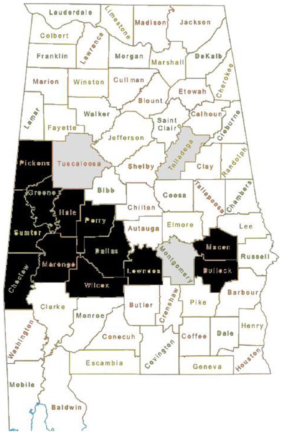
Division map of Alabama.

Two approaches, one employing partial equilibrium models and the other CGE models, are often used in regional economic analyses. To represent complicated economic relationships, partial equilibrium analyses, which often focus on specific sectors and ignore the rest of the economy, are insufficient. Therefore, it is necessary to build up a CGE model that handles an economy as a whole.

A CGE model looks at the economy as a complete system of interdependent components. It consists of a number of equations that represent the complex relationships among various variables and a database consistent with the equations. This approach is generally based on comparative static analysis in which the base equilibrium is compared with the new equilibrium after the exogenous shocks have taken place. It is widely used in economy-wide impact analysis, in particular when the transmission channels are complex. Recently, the CGE approach has also been used in regional policy analyses (Partridge & Rickman, 2007). Unlike partial equilibrium models, CGE models take into account the interindustry linkages, since the models intend to model all linkages in an economy. Compared with partial equilibrium analysis, CGE models’ accounting and theoretical consistency make these models a valuable tool to conduct interindustry analysis and welfare analysis. Therefore, the CGE approach¹⁰ is deemed a more proper framework for implementing economic impact analyses. As such, we have chosen it to investigate the automotive sector’s impact on the Alabama economy.

The CGE model (aggregation scheme for the Alabama regional economy; see Table 1)¹¹ in this study is modified and based closely on the CGE model constructed by Stodick, Holland, and Devadoss (2004) and also by Löfgren (2000). The model (see the appendix), which was originally used in tax analysis in Washington, D.C., can also be extended to do the likely economic analyses. In this study, a regional CGE model was constructed for Alabama’s auto-plant-based counties, for the Black Belt, and for the entire state of Alabama. The PATH solver, which relies on GAMS software, is applied to generate and solve simultaneous nonlinear equations in the CGE model. Five blocks, consisting of households, firms, government, trade, and macro closures, are presented in the following subsections.

Table 1.

The Aggregation Scheme for the Alabama Regional Economy.

Sectors	Aggregated individual IMPLAN sector codes
Agriculture	1-19
Auto	276-277, 279,283
Auto parts	320, 362, 414-415
Auto, horizontal	278, 280-282, 292-294
Construction	34-40
Manufacturing	41-291, 295-318
Mining	20-30
Trade	319
Service	321-331, 336-361, 363-427
Transportation	332-335
Utility	31-33
Miscellaneous	428-440

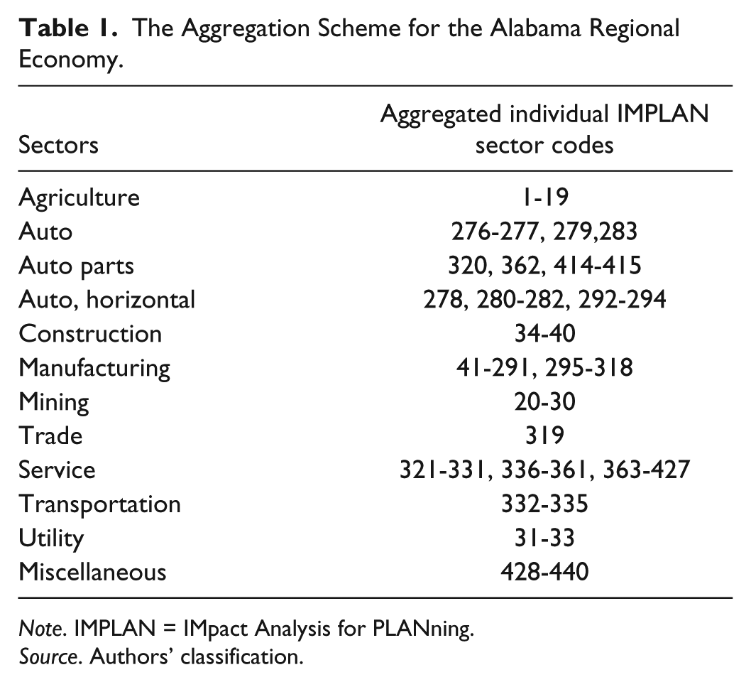
Note. IMPLAN = IMpact Analysis for PLANning.

Source. Authors’ classification.

Households

IMPLAN provides data for nine distinct household groups based on income levels. A representative household in each category is assumed to maximize the Stone–Geary utility function by choosing its optional consumption bundle. This study also assumes that the household budget consists of income and consumption expenditure, and the endowment of household includes capital and labor. Moreover, the sources of household income revenues are returns on primary factors, transfers from the governments, other households, the rest of United States, and the rest of the world. Each household allocates its consumption expenditure to private consumptions, taxes, and savings.

Firms

In this study, each sector is aggregated by many firms but is regarded as a single representative firm assumed to produce a homogeneous product according to a nested production function. The representative firm’s problem is to maximize its profits subject to its budget constraints.

Two levels are formulated in the production process: the production of composite goods and the production of gross output. At the first level, two primary factors, labor and capital, are employed in the constant elasticity of substitution (CES) production process to produce the composite goods. At the second level, the firms use the intermediate inputs with the composite goods to produce the final goods under Leontief technology.

The elasticity of substitution between labor and capital¹² for each industry is borrowed from de Melo and Tarr (1992). Given that there is little guidance about the determination of the supply elasticities of labor and capital, following Holland and Razack (2006), we assume that the supply elasticity of labor is set to 2.0 and the supply elasticity of capital is set to 1.0 in the medium run for all regions, whereas in the short run, both supply elasticities of labor and capital are set to 0.5.

Government

As specified in IMPLAN, the government in this model has two levels:¹³ (a) the federal government and (b) a combination of state and local government. This study has attempted to do the same by dividing the government into two levels. Governments are assumed to balance their budgets and to affect the economy mainly through two ways: taxation and government spending. Taxation includes income taxes on households, investment, and indirect taxes that are levied from production activities and tariffs. Government spending consists of government consumption, government savings, transfers to households, and payments to foreign nations. Like households and firms, governments can lend or borrow as well.

Trade

To analyze a regional economy within a country, it is necessary to take into consideration its connection to the rest of the country and the world. As a result, both domestic trade and international trade are implicitly included in this model. In other words, a representative firm sells its products outside of the region within the United States, and some of the products are also sold outside of the United States. The Armington assumption¹⁴ was used to differentiate between domestic and imported goods, which are an imperfect substitute for each other. Given the two kinds of trade, we used a two-level Armington function. In the first level, regionally produced goods were distinguished from domestically imported goods, as they are imperfect substitutes for each other; in the second level, substitution between domestic imports and foreign imports is allowed.

The constant elasticity of transformation (CET)¹⁵ function is used to decide the production possibility of the choice between domestic goods and export goods. Like the CES function, the CET function also has a two-level structure: It not only differentiates between exported goods and domestically consumed goods but also distinguishes between exports to the rest of United States and those to the rest of the world. Contrary to the parameters adopted by most regional CGE modelers, the salient feature of this study is that it uses disparate elasticities on different levels, which overcomes the weakness pointed out by Partridge and Rickman (2007), who contend that routine use of the national substitution elasticities in regional economic development analysis would degrade the results obtained. Since the regional economy is more open than the national economy and the wide range for elasticities is specified in different sources, the elasticities in regional analyses usually have higher values. In contrast, the elasticities of substitution for regional analyses are smaller than those on the national level in analyses (Holland, 2010). Figure 2 illustrates the structure of production and trade. However, given the unavailability of the CES and CET elasticities for the Alabama economy, the values of the CES and CET elasticities used in this study are based on estimates as specified in de Melo and Tarr (1992) and Berck and Golan (1997) and are listed in Table 2. The central elasticity values estimated for the related industries are used in this analysis. Since the elasticities adopted cannot precisely reflect the structure of the Alabama economy, the simulation results would diverge from their real values. Hence, a number of sensitivity experiments will be conducted in the section titled “Sensitivity Analysis.”

Figure 2.

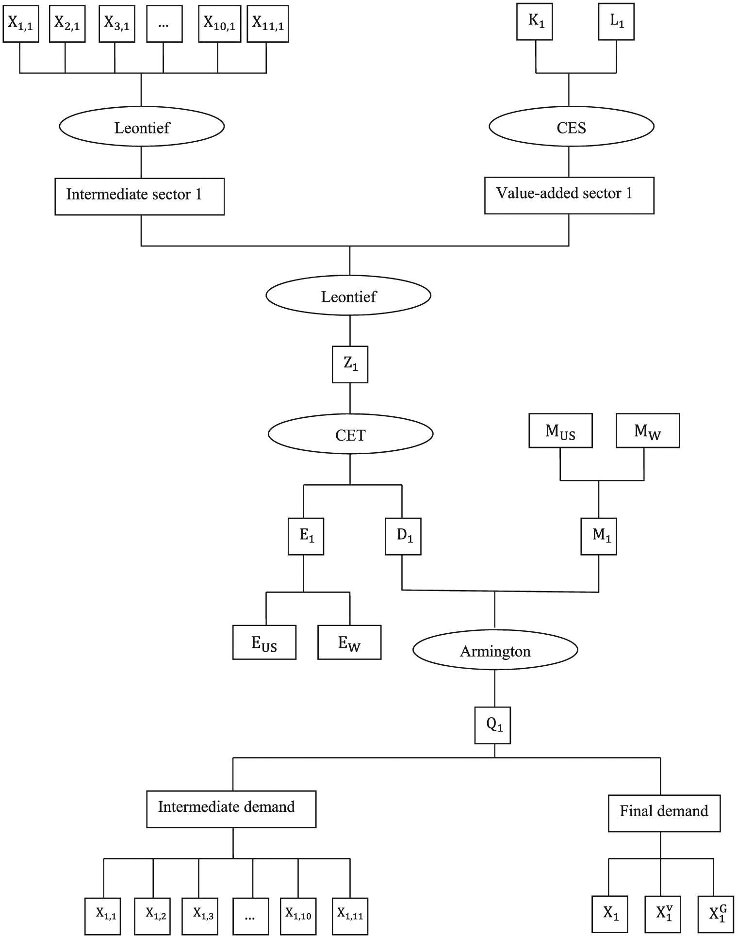
The production and trade structure, taking the first sector as an example.

Table 2.

Elasticity Values in Alabama CGE Model.

Elasticity	Value
Elasticity of substitution between regional output and imports
Agriculture	1.42
Automotive	2.01
Construction	2.86
Manufacturing	3.55
Mining	0.50
Others	2.00
Elasticity of substitution between imports (rest of world) and imports (rest of United States)
Agriculture	1.99
Automotive	8.39
Construction	2.86
Manufacturing	6.97
Mining	1.1
Others	4.0
Elasticity of substitution between domestic and foreign demand
Agriculture	5.2
Automotive	4.2
Trade, service	1.1
Others	4.2
Elasticity of substitution between exports (rest of world) and exports (rest of United States)
Agriculture	3.9
Automotive	2.9
Trade, service	0.7
Others	2.9

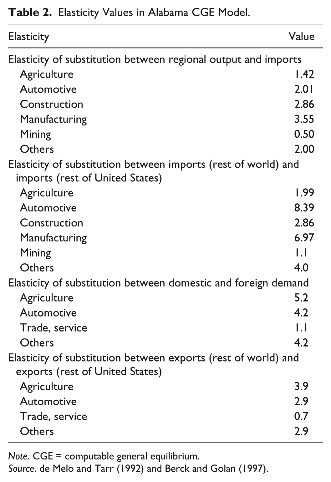
Note. CGE = computable general equilibrium.

Source. de Melo and Tarr (1992) and Berck and Golan (1997).

Macro Closures

There is no clear evidence regarding how long it takes for an economy to reach an equilibrium following a shock. Following Rickman (1992) and Waters, Holland, and Weber (1997), we applied two popular closures,¹⁶ neoclassical and Keynesian, to the model. Neoclassical closure is often used in short-run analyses (1-2 years), while Keynesian closure is applied to medium-run analyses (3-5 years).

Neoclassical closure assumes that the labor supply and capital supply are fixed, so only the wage rate and the capital rent rate can be adjusted to clear the factor markets. Although Keynesian closure specifies the same capital supply, it assumes that the labor supply is perfectly elastic and the wage rate is fixed. In the neoclassical closure, investment is endogenous, so it is determined by various kinds of savings. In contrast, under the Keynesian closure, saving is endogenous, so the Keynesian model is considered the investment-driven model.

Under either specification, a set of prices will clear both factor markets and commodity markets. The factor-market equilibrium requires that the employed factors in each sector equal their endowment. The commodity-market equilibrium requires that the supply of each commodity equals the demand of each commodity. In addition, the CPI is treated as the numeraire in this study.

Empirical Result and Analysis

The aim of this section is to identify the impact of the auto export expansion on economic growth and explore whether communities in the Black Belt receive economic benefits from increased auto export shocks. Suppose that Alabama exports all of its produced vehicles, either to other states in the United States or abroad. Given an already established industry, a hypothetical 5%¹⁷ year-to-year increase in auto export demand is assumed to investigate its potential impact. We consider this figure to be reasonable, as it reflects the magnitude of the auto production growth in Alabama. To simplify the analysis, this study further assumes that the auto export demand increases 5% for both domestic and international trade. Therefore, we have two simulation scenarios: one in which we shock the model by increasing the auto export demand by 5% in the short run; the other in which we increase auto export demand by 5% in the medium run. Tables 3 through 7 present the simulation results, which are in percentage terms with the exception of the numbers in the lower panel of Table 6, which are presented in quantity changes. We must also note that for display purposes, we aggregate nine households into three groups. This study considers a household whose income is over $75,000 as a high-income household, a household whose income ranges from $25,000 to $75,000 as a middle-income household, and a household whose income is under $25,000 as a low-income household.

Table 3.

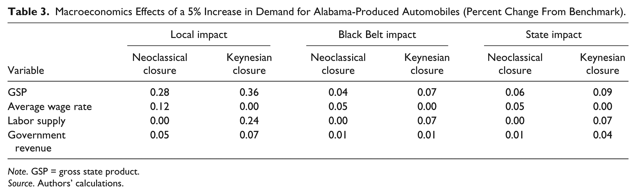
Macroeconomics Effects of a 5% Increase in Demand for Alabama-Produced Automobiles (Percent Change From Benchmark).

Variable	Local impact		Black Belt impact		State impact
Variable	Neoclassical closure	Keynesian closure	Neoclassical closure	Keynesian closure	Neoclassical closure	Keynesian closure
GSP	0.28	0.36	0.04	0.07	0.06	0.09
Average wage rate	0.12	0.00	0.05	0.00	0.05	0.00
Labor supply	0.00	0.24	0.00	0.07	0.00	0.07
Government revenue	0.05	0.07	0.01	0.01	0.01	0.04

Note. GSP = gross state product.

Source. Authors’ calculations.

Table 4.

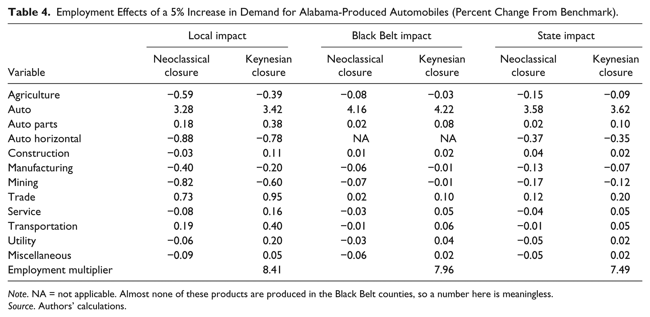
Employment Effects of a 5% Increase in Demand for Alabama-Produced Automobiles (Percent Change From Benchmark).

Variable	Local impact		Black Belt impact		State impact
Variable	Neoclassical closure	Keynesian closure	Neoclassical closure	Keynesian closure	Neoclassical closure	Keynesian closure
Agriculture	−0.59	−0.39	−0.08	−0.03	−0.15	−0.09
Auto	3.28	3.42	4.16	4.22	3.58	3.62
Auto parts	0.18	0.38	0.02	0.08	0.02	0.10
Auto horizontal	−0.88	−0.78	NA	NA	−0.37	−0.35
Construction	−0.03	0.11	0.01	0.02	0.04	0.02
Manufacturing	−0.40	−0.20	−0.06	−0.01	−0.13	−0.07
Mining	−0.82	−0.60	−0.07	−0.01	−0.17	−0.12
Trade	0.73	0.95	0.02	0.10	0.12	0.20
Service	−0.08	0.16	−0.03	0.05	−0.04	0.05
Transportation	0.19	0.40	−0.01	0.06	−0.01	0.05
Utility	−0.06	0.20	−0.03	0.04	−0.05	0.02
Miscellaneous	−0.09	0.05	−0.06	0.02	−0.05	0.02
Employment multiplier		8.41		7.96		7.49

Note. NA = not applicable. Almost none of these products are produced in the Black Belt counties, so a number here is meaningless.

Source. Authors’ calculations.

Table 5.

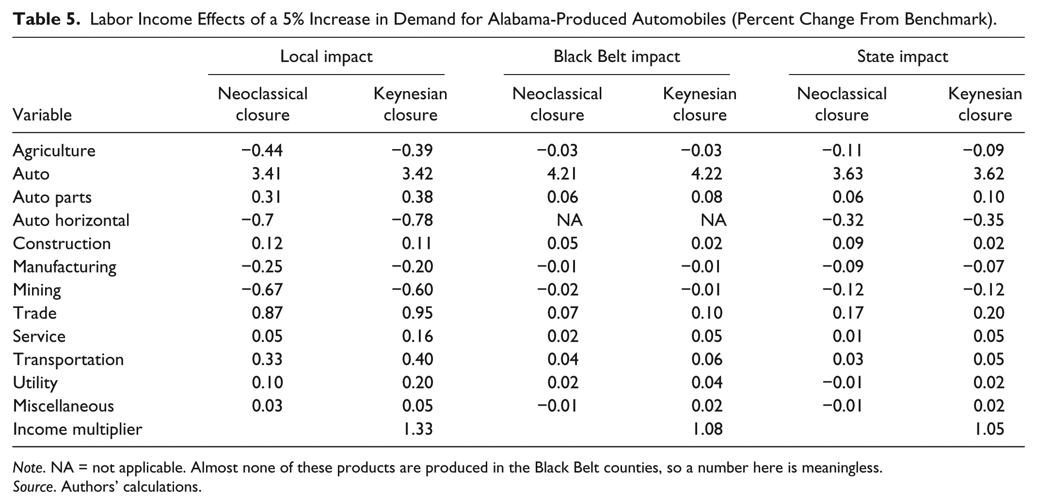
Labor Income Effects of a 5% Increase in Demand for Alabama-Produced Automobiles (Percent Change From Benchmark).

Variable	Local impact		Black Belt impact		State impact
Variable	Neoclassical closure	Keynesian closure	Neoclassical closure	Keynesian closure	Neoclassical closure	Keynesian closure
Agriculture	−0.44	−0.39	−0.03	−0.03	−0.11	−0.09
Auto	3.41	3.42	4.21	4.22	3.63	3.62
Auto parts	0.31	0.38	0.06	0.08	0.06	0.10
Auto horizontal	−0.7	−0.78	NA	NA	−0.32	−0.35
Construction	0.12	0.11	0.05	0.02	0.09	0.02
Manufacturing	−0.25	−0.20	−0.01	−0.01	−0.09	−0.07
Mining	−0.67	−0.60	−0.02	−0.01	−0.12	−0.12
Trade	0.87	0.95	0.07	0.10	0.17	0.20
Service	0.05	0.16	0.02	0.05	0.01	0.05
Transportation	0.33	0.40	0.04	0.06	0.03	0.05
Utility	0.10	0.20	0.02	0.04	−0.01	0.02
Miscellaneous	0.03	0.05	−0.01	0.02	−0.01	0.02
Income multiplier		1.33		1.08		1.05

Note. NA = not applicable. Almost none of these products are produced in the Black Belt counties, so a number here is meaningless.

Source. Authors’ calculations.

Table 6.

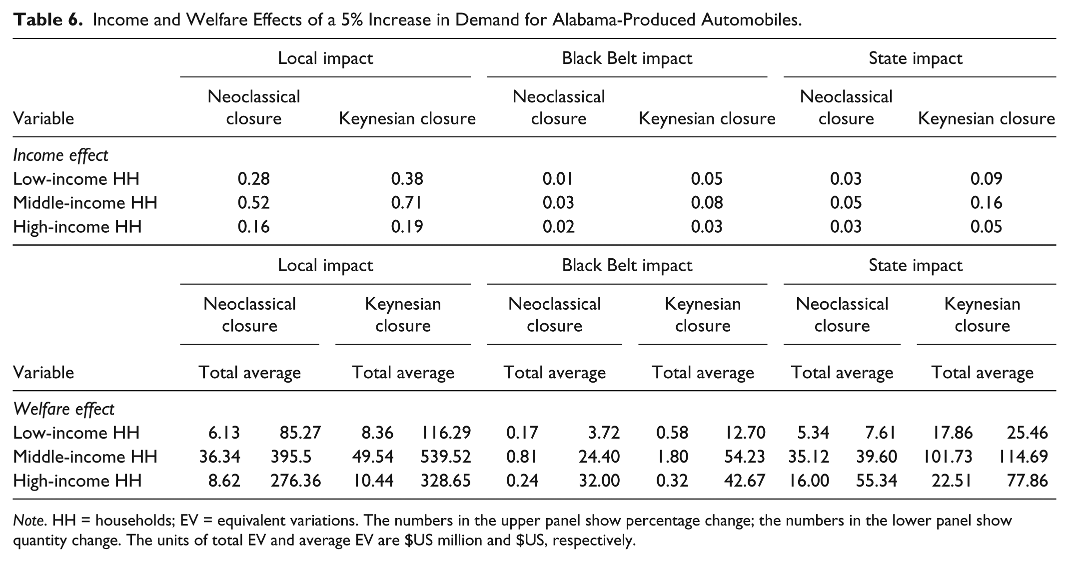
Income and Welfare Effects of a 5% Increase in Demand for Alabama-Produced Automobiles.

Variable	Local impact				Black Belt impact				State impact
Variable	Neoclassical closure		Keynesian closure		Neoclassical closure		Keynesian closure		Neoclassical closure		Keynesian closure
Income effect
Low-income HH	0.28		0.38		0.01		0.05		0.03		0.09
Middle-income HH	0.52		0.71		0.03		0.08		0.05		0.16
High-income HH	0.16		0.19		0.02		0.03		0.03		0.05
Variable	Local impact				Black Belt impact				State impact
	Neoclassical closure		Keynesian closure		Neoclassical closure		Keynesian closure		Neoclassical closure		Keynesian closure
	Total average		Total average		Total average		Total average		Total average		Total average
Welfare effect
Low-income HH	6.13	85.27	8.36	116.29	0.17	3.72	0.58	12.70	5.34	7.61	17.86	25.46
Middle-income HH	36.34	395.5	49.54	539.52	0.81	24.40	1.80	54.23	35.12	39.60	101.73	114.69
High-income HH	8.62	276.36	10.44	328.65	0.24	32.00	0.32	42.67	16.00	55.34	22.51	77.86

Note. HH = households; EV = equivalent variations. The numbers in the upper panel show percentage change; the numbers in the lower panel show quantity change. The units of total EV and average EV are $US million and $US, respectively.

Table 7.

Sensitivity Analysis of Changes in the Factor Substitution Elasticity and the Export Demand Elasticity.

Variable	Local impact				Black Belt impact				State impact
	Neoclassical closure		Keynesian closure		Neoclassical closure		Keynesian closure		Neoclassical Closure		Keynesian closure
	α = −2	α = −5	α = −2	α = −5	α = −2	α = −5	α = −2	α = −5	α = −2	α = −5	α = −2	α = −5
GSP	0.42	0.28	0.49	0.36	0.06	0.04	0.08	0.07	0.09	0.06	0.12	0.09
Average wage rate	0.19	0.12	0.00	0.00	0.07	0.05	0.00	0.00	0.07	0.05	0.00	0.00
Labor supply	0.00	0.00	0.47	0.24	0.00	0.00	0.08	0.07	0.00	0.00	0.10	0.07
Govt. revenue	0.07	0.05	0.09	0.07	0.01	0.01	0.01	0.01	0.02	0.01	0.03	0.04
Low-income HH EV	8.95	6.13	11.30	8.36	0.25	0.17	0.69	0.58	7.74	5.34	23.86	17.86
Middle-income HH EV	52.94	36.34	66.93	49.54	1.12	0.81	2.12	1.80	50.21	35.12	133.07	101.73
High-income HH EV	12.57	8.62	14.02	10.44	0.33	0.24	0.37	0.32	22.77	16.00	28.77	22.51
	ρ = 0.5	ρ = 0.81	ρ = 0.5	ρ = 0.81	ρ = 0.5	ρ = 0.81	ρ = 0.5	ρ = 0.81	ρ = 0.5	ρ = 0.81	ρ = 0.5	ρ = 0.81
GSP	0.28	0.28	0.36	0.36	0.04	0.04	0.07	0.07	0.06	0.06	0.09	0.09
Average wage rate	0.12	0.12	0.00	0.00	0.05	0.05	0.00	0.00	0.05	0.05	0.00	0.00
Labor supply	0.00	0.00	0.24	0.24	0.00	0.00	0.07	0.07	0.00	0.00	0.07	0.07
Govt. revenue	0.05	0.05	0.07	0.07	0.01	0.01	0.01	0.01	0.01	0.01	0.03	0.04
Low-income HH EV	6.12	6.13	8.36	8.36	0.18	0.17	0.58	0.58	5.34	5.34	17.85	17.86
Middle-income HH EV	36.30	36.34	49.53	49.54	0.81	0.81	1.80	1.80	35.13	35.12	101.65	101.73
High-income HH EV	8.60	8.62	10.44	10.44	0.24	0.24	0.32	0.32	16.00	16.00	22.48	22.51

Note. GSP = gross state product; HH = households. All variables are present in percentage changes except the three total equivalent variations (EV).

Macroeconomic Effects

Table 3 presents the percentage changes in selected macroeconomic variables from the 5% hypothetical increase in the auto demand. These changes occur under different model specifications with varying assumptions about the labor-market adjustment and capital mobility. An overview of the results demonstrates that the demand shocks have entirely different impacts on different parts of Alabama. That is, although auto expansion has a tremendous impact on automobile-based counties, it has a much smaller impact on the Black Belt and on the state as a whole.

Under neoclassical closure theory, total labor supply is fixed in each specific region. Hence, firms can only adjust the wage rates in response to the expanding auto demand, so the percentage change of labor supply is zero. As expected, auto-plant counties are the biggest gainers from the auto boom in terms of percentage changes in GSP, average wage rate, labor supply, and government revenue. In contrast, the auto boom’s impact on the Black Belt areas and on the entire state is limited. For example, the expanding demand for automobiles lifts GSP by 0.28% in the auto-plant counties, as opposed to only 0.04% for the Black Belt counties and 0.06% for the state, as shown in Table 2. Because of regional spillover effects, the entire state as well as the Black Belt area benefits from the increased auto demand: GSP, the wage rate, and government revenue rise by 0.04%, 0.05%, and 0.01%, respectively, for Black Belt counties. Comparing the percentage changes in GSP for auto-plant-based counties and Black Belt counties, we find that the local impact is seven times as great for counties with auto plants as for the Black Belt counties. Turning to the state impact, the tiny effect of increased demand for autos on GSP is unsurprising; it stems from the fact that the automotive industry only accounts for 2% of GSP in Alabama.

Under the Keynesian specification in which firms adjust their employment in response to increased demand for autos, the picture changes. The economic model adjusts the number of workers instead of the wage rate, which is fixed to reflect wage rigidity. As a result, if auto labor demand rises, workers from other regions will migrate into the region. Otherwise, labor forces will migrate out of the region. Compared with the short-run neoclassical CGE, this increased demand for autos has a greater impact on each of those macroeconomic variables. For example, GSP and government revenue rise by 0.36% and 0.07% for auto-plant-based counties, 0.07% and 0.01% for Black Belt counties, and 0.09% and 0.04% for Alabama as a whole, as opposed to 0.28% and 0.05%, 0.04% and 0.01%, and 0.06% and 0.01% under the neoclassical specification. All three regions are better off in the Keynesian closure than in the neoclassical closure, but the impact on Black Belt counties and the statewide impact are still small in the medium run. These results also imply that Alabama is not overly dependent on its automotive industry. In sum, the overall impact of auto expansion is definitely positive but disproportionate from a macroeconomic perspective.

Impact on Employment

Table 4 indicates a mixed picture of the employment effects resulting from the expansion in demand for autos.

In the short run, the labor force is fixed in respective regions, so the increased auto demand can only draw labor from other industries in the same region. Nonetheless, in response to auto export expansion, higher wages in the automotive industry can easily drive workers from the horizontal automotive industry, considering the similar skills and backgrounds required by both sectors. As expected, the automotive industry is the biggest job gainer. Although under the neoclassical closure model the automotive industry experiences a moderate increase (around 4%) in employment regardless of the area we examine, most industries experience job losses in all three regions. The job losses mainly concentrate on the agriculture industry, manufacturing industry, mining industry, and horizontal auto industry in terms of percentage changes. Specifically, the horizontal automobile industry is most negatively affected by the increased automobile demand, which attracts workers with similar skills from other industries to the automotive sector, resulting in a loss of 0.88% in the auto-plant counties and of 0.37% in the entire state of Alabama.

In the medium run, the labor force is interregionally mobile and wage rates are fixed. Under these assumptions, the increased auto demand not only brings about employment in the auto industry but also job gains in the other industries. However, its impact on employment in nonautomotive industries is tiny for the Black Belt. As shown in Table 4, it is evident that most industries have experienced job increases. Besides benefiting the workers in the automotive industry, the employment effects of the automotive sector also extend to workers who are not directly participating in any auto-making activities, which highlights the sectoral spillover effects. For example, the trade, service, and transportation industries increase slightly—by 0.10%, 0.05%, and 0.06%, respectively—in employment for Black Belt counties. Moreover, as indicated in Table 4, the employment multipliers for auto-plant-based counties, Black Belt counties, and the entire state are 8.41, 7.96, and 7.49, respectively. It is interesting to note that except for the auto-plant-based counties, the employment multiplier is larger for the Black Belt areas than for the state of Alabama. It is also worth noting that in both the short and the medium run, auto expansion has a larger employment impact (4.22%) on the auto industry in Black Belt counties than in local counties (those with auto plants) or in the entire state.

Labor Income Effects

Table 5 indicates the labor income effects caused by the increased demand for autos. As expected, for most industries, the medium-run effects are more likely to be positive and larger than the short-run effects. Again, the reason is that labor supply is fixed in the short run, whereas in the medium run, labor forces are mobile across regions and unemployment exists. Increased auto demand not only attracts workers from other industries, it also attracts the unemployed.

Apparently, as shown in Table 5, the labor income of the auto industry increases more rapidly than that in other sectors, while the horizontal auto industry undergoes losses in those regions. Labor income increases 3.41%, 4.21%, and 3.63% for our three regions. Again, Black Belt counties enjoy the largest increase. Furthermore, some industries—such as the utility industry—that are adversely affected under the neoclassical closure are positively influenced under the Keynesian specification, but not vice versa. The income multipliers for the three regions are 1.33, 1.08, and 1.05, respectively, as shown in Table 5. Interestingly, the negative effects to most industries under the neoclassical specification are mitigated when they are examined under the Keynesian closure, excluding the horizontal auto industry. Take the labor incomes in the agricultural industry as an example: These incomes changed from −0.44%, −0.03%, and −0.11% to −0.39%, −0.03%, and −0.09%, respectively, for the three regions.

Overall, the figures in Table 5 imply that the auto expansion’s effect on labor income is small, especially on the nonauto industries. From a policy point of view, as a newly established industry, its impact on the economy is still limited. We also note that, under the Keynesian closure, the percentage changes of labor incomes in Table 4 are the same as the percentage changes of employment in Table 5. Given that the wage rates are fixed in the medium run, the firms adjust the employment in response to the auto demand, which results in the same changes in employment and labor incomes.

Income and Welfare Effects

Table 6 demonstrates the income effects and the welfare changes that are measured by equivalent variation (hereafter referred to as “EV”), which accounts for changed price effects for each household category in all regions. The welfare changes reflect how much better off the households would be from the rise in auto export demand. Unlike the income measure, it takes both price changes and income changes into account.

An overview of Table 6 indicates that both income effects and welfare effects are positive regardless of the regions we examine. Further analysis of the results from both the upper panel and the lower panel of Table 6 allows us to generalize about the following three results:

The income gain and welfare gain are not distributed evenly across regions and households. Middle-income households experience the largest income increase in all regions. Take the households in the Black Belt as an example: The income increase for middle-income households is 0.03% and 0.08%, respectively, under those two closures, as opposed to 0.01% and 0.05% for low-income households and 0.02% and 0.03% for high-income households. When it comes to regional differences, as expected, the households from the auto-plant counties enjoyed the largest income increase under both closures. From the lower panel, we see similar results: Middle-income households tend to receive the most benefits from the auto boom in terms of welfare change, and so do households from auto-plant counties. Moreover, we can find obvious regional differences. For instance, the welfare gain of the households from the auto-plant-based counties is much larger than that of the households from neighboring counties in terms of average EV (obtained by dividing the total EV by the number of households). For example, in the medium run, the income from welfare payments to the poorest households from auto-plant-based countries increases by $116.29. In contrast, for households from the Black Belt and other regions in Alabama, welfare payments increase by only $12.70 and $25.46, respectively. Thus, we arrive at the conclusion that the auto export expansion contributes to relieving poverty in the auto-plant-based counties but that for the other counties, especially the Black Belt counties, its effectiveness is rather limited.

The medium-run effect is larger than the short-run effect. By comparing the numbers in the neoclassical closure column with those in the Keynesian closure column, we can easily reach this conclusion. The finding is particularly important for policy makers when coming up with a relevant development strategy.

The crippling effect on residents stemming from the auto export expansion extends to the Black Belt counties. It may be noted that in the medium run, the total welfare impact ($580,000) on low-income households is larger than that ($320,000) on high-income households. Total welfare impact on low-income households is also larger than that on high-income households in the Black Belt counties, but the opposite is true for the average welfare effect. Given the larger welfare impact existing in the middle- and high-income households, we see that the wealth gap in the Black Belt region became wider after the shocks.

Sensitivity Analysis

From a policy-analysis standpoint, one of the major problems of the CGE modeling approach is the reliability of the model. Because of the heavy dependence on elasticities in the literature, sensitivity analyses should be undertaken on certain elasticities to assess the robustness of the model. Although not reported here, a series of systematic sensitivity analyses were done. In particular, the results of two sensitivity experiments are reported here. First, we examine the sensitivity to a changed elasticity of factor substitution ρ between labor and capital in the automotive industry. Second, we explore the model’s sensitivity to the changed export demand elasticity α.

The factor substitution elasticity between labor and capital for the automotive industry used in the simulation is from de Melo and Tarr (1992). The value of 0.81 is referred to as the “central” value. Given that the value is not estimated for the Alabama automotive industry in particular, and given also Alabama’s high-quality labor force, the low estimate value of 0.50 from de Melo and Tarr (1992) was used as an alternative to test the robustness of the model. The original export demand elasticity is assumed to be −5. By changing its value to −2 for the purpose of comparison, the model’s sensitivity to the export demand elasticity can be examined. Parts of the results¹⁸ are summarized in Table 7.

The findings presented in Table 7 demonstrate that two different factor substitution elasticities between labor and capital in the automotive sector generate almost entirely the same results. This implies the model’s strong robustness to the choice of factor substitution elasticities. The results from Table 7 also indicate that the simulation results are insensitive to the changes in the value of export demand elasticity. Based on the results obtained from a series of sensitivity tests, we can conclude that our CGE model is robust. Therefore, the simulation results obtained from the model are reliable.

Conclusion

The study we have undertaken is an attempt to measure the contribution of the automotive industry to the Alabama economy. Impacts of auto demand shocks are examined under two model specifications. A general equilibrium analysis on the auto industry generates a number of important conclusions.

First, the most important finding shows that Alabama’s automotive industry has a disproportionate impact across Alabama. The impact of the expansion of auto exports on the auto-plant-based counties is strong, but Black Belt counties and the state as a whole also receive economic benefits from the auto boom, though to a lesser extent. Benefits accrue primarily to counties in which the auto plants and their suppliers are located. The spillover effects into nonautomobile counties are modest and about evenly distributed.

Second, middle-income households are the largest gainers, and this is true across all counties, including the Black Belt counties, where poverty is concentrated. Despite its rapid growth, the auto industry continues to constitute a small fraction of the state’s economy (less than 3% of GSP). Thus, overdependence on a cyclical industry is as yet not an issue for policy makers.

Third, the Keynesian closure produced larger impacts than the neoclassical closure.

Finally, sensitivity analyses indicate that our findings are reliable, since the model is robust to the elasticities that were borrowed from the literature.

This study fills a gap in the literature, since it empirically investigates the economic contribution of the automotive industry to Alabama’s economy as well as to the economy of the Black Belt counties within the state. In contrast to extant studies, it also complements the literature by using the regional CGE methodology. Given that the automotive industry accounts for roughly 2% of GSP, that industry plays a less important role in the Alabama economy than expected. Although its impact on the auto-plant-based counties is apparent, for Black Belt counties the impact is modest.

In light of this, it is apparent that to further develop the Alabama economy and help relieve the poverty in the Black Belt counties, it is not enough for state officials to rely on the automotive industry. Our results indicate that Alabama has to carefully craft its development strategy. It cannot continue to depend on promoting exports such as automotive sales, as has been articulated in government development plans. Instead, sustained efforts should be made toward further integration between rural and urban regions by strengthening rural–urban partnerships. This integration consists of a number of linkages. Improvement of these market and nonmarket links would lift the development of both rural and urban regions, since the different assets of these regions can potentially complement one another (Organisation for Economic Co-operation and Development, 2013).

Moreover, this study also presents some valuable conclusions to aid policy makers in identifying not only the affected stakeholders in the expansion of demand for automobile exports but also the direction and magnitude resulting from the auto demand shocks. Finally, the empirical findings here also have implications for other Southern auto states where auto manufacturing plays an increasingly important role, such as South Carolina, Mississippi, and Tennessee, all of which have attracted new foreign-owned assembly plants since 1990.

Footnotes

Appendix

This section presents the parameters, variables, and equations used in the Alabama CGE model.

A = activities

C = commodities

CM⊂C = commodities that have at least one source of imports (from Rest of World [RoW], from Rest of United States [RUS], or from both)

CE⊂C = commodities that have at least one destination for exports (to RoW, to RUS, or to both)

CNM⊂C = commodities that are not imported

CNE⊂C = commodities that are not exported

CM1⊂C = commodities that have exactly one import source

CE1⊂C = commodities that have exactly one export destination

CM2⊂C = commodities that are imported from both sources

CE2⊂C = commodities that are exported to both destinations

F = factors of production and indirect business taxes

FF⊂F = factors of production

I = institutions

H⊂I = households

G⊂I = government units

HG⊂I = households and government units

FG⊂G = federal government units

SG⊂G = state government units

T = trading regions (FT: Rest of World; DT: Rest of US)

FF = FFF, C = CC, H = HH, G = GG, FG = FGG, SG = SGG

Declaration of Conflicting Interests

The author(s) declared no potential conflicts of interest with respect to the research, authorship, and/or publication of this article.

Funding

The author(s) disclosed receipt of the following financial support for the research, authorship, and/or publication of this article: The authors received Alabama Agricultural Experiment Station (AAES) financial support for this research.

Notes

Author Biographies

Lei Zhang, PhD, is an assistant professor at the Center for Economic Research, Shandong University. His research has been published in Energy Economics, African Development Review, and in Frontiers of Economics in China.

Henry Kinnucan, PhD, is an alumni professor and graduate director in the Department of Agricultural Economics and Rural Sociology, Auburn University, Auburn, Alabama. His research interests include agricultural prices, marketing, trade, and rural development.

Jing Gao, PhD, is an assistant professor in the International School of Economics and Management at Capital University of Economics and Business. Her research has been published in Energy Economics and Journal of Business Economics and Statistics.

References

Alabama Automotive Manufacturers Association. (2008). Alabama’s automotive manufacturing industry continues growth (Press release). Birmingham, AL: Author.

Azariadis

Stachurski

(2005). Poverty traps. In Aghion

Durlauf

S. N.

(Eds.), Handbook of economic growth (Vol. 1, pp. 295-384). Amsterdam, Netherlands: North Holland.

Berck

Golan

(1997). State tax policy, labor, and tax revenue feedback effects. Industrial Relations: A Journal of Economy and Society, 36, 399-418.

Blonigen

B. A.

Wilson

W. W.

(1999). Explaining Armington: What determines substitutability between home and foreign goods? Canadian Journal of Economics, 32, 1-21.

Cali

Menon

(2012). Does urbanization affect rural poverty? Evidence from Indian districts. World Bank Economic Review, 27, 171-201.

Center for Automotive Research. (2004). Contribution of the U.S. motor vehicle industry to economies of the United States, California, New York, and New Jersey in 2003. Retrieved from http://irlee.umich.edu/clmr/Docs/Impact-AutoInd-US-CA-NY-NJ-2003.pdf

Center for Automotive Research. (2008). CAR research memorandum: The impact on the U.S. economy of a major contraction of the Detroit Three automakers. Ann Arbor, MI: Author.

Center for Automotive Research. (2010). Contribution of the automotive industry to the economies of all fifty states and the United States. Ann Arbor, MI: Author.

de Melo

Tarr

D. G

. (1992). A general equilibrium analysis of US foreign trade policy. Cambridge: MIT Press.

10.

Economic Development Partnership of Alabama. (2009). Alabama’s automotive industry, 2009. Birmingham, AL: Author.

11.

Economic Development Partnership of Alabama. (2012). Alabama’s automotive industry, 2012. Birmingham, AL: Author.

12.

Ellison

Glaeser

E. L.

(1997). Geographic concentration in U.S. manufacturing industries: A dartboard approach. Journal of Political Economy, 105, 889-927.

13.

Foster

A. D.

Rosenzweig

M. R.

(2004). Agricultural productivity growth, rural economic diversity, and economic reforms: India, 1970-2000. Economic Development and Cultural Change, 52, 509-542.

14.

Fox

Sohnesen

T. P.

(2012). Household enterprises in Sub-Saharan Africa: Why they matter for growth, jobs, and poverty reduction. Washington, DC: World Bank.

15.

Greenstone

Hornbeck

Moretti

(2010). Identifying agglomeration spillovers: Evidence from winners and losers of large plant openings. Journal of Political Economy, 118, 536-598.

16.

Haddad

E. A.

Hewings

G. J.

(1999). The short-run regional effects of new investments and technological upgrade in the Brazilian automobile industry: An interregional computable general equilibrium analysis. Oxford Development Studies, 27, 359-383.

17.

Haggblade

Hazell

P. B.

Dorosh

P. A.

(2007). Sectoral growth linkages between agriculture and the rural nonfarm economy. In Haggblade

Hazell

Reardon

(Eds.), Transforming the rural nonfarm economy: Opportunities and threats in the developing world (pp. 141-182). Baltimore, MD: Johns Hopkins University Press.

18.

Holland

(2010). What happens when exports expand: Some ideas for closure of regional computable general equilibrium models. Annals of Regional Science, 45, 439-451.

19.

Holland

Razack

(2006, September). Assessing the economic impact of an agricultural export shock on the Washington economy: A tale of two models (Working Paper No. 2006-11). Pullman: Washington State University, School of Economic Sciences.

20.

Information Handling Services. (2013). The economic impact of the motor vehicle parts manufacturing industry on the United States (Prepared for the Motor and Equipment Manufacturers Association). Washington, DC: Author.

21.

International Institute for Environment and Development. (2009). Urbanisation and rural-urban linkages. London, England: Author.

22.

Jacobs

A. J.

(2012). Collaborative regionalism and foreign direct investment: The case of the Southeast automotive core and the “new domestics.” Economic Development Quarterly, 26, 199-219.

23.

Kebede

Ngandu

M. S.

(1999). The economic impact of the Mercedes Benz investment on the state of Alabama. Journal of Agricultural and Applied Economics, 31, 371-382.

24.

Kline

Moretti

(2014). Local economic development, agglomeration economies, and the big push: 100 Years of evidence from the Tennessee Valley Authority. Quarterly Journal of Economics, 129, 275-331.

25.

Kraybill

D. S.

(1993). Computable general equilibrium analysis at the regional level. In Otto

D. M.

Johnson

T. G.

(Eds.), Microcomputer-based input-output modeling: Applications to economic development (pp. 125-148). Boulder, CO: Westview.

26.

Lanjouw

J. O.

Lanjouw

(2001). The rural non-farm sector: Issues and evidence from developing countries. Agricultural Economics, 26, 1-23.

27.

Löfgren

(2000). Exercises in general equilibrium modeling using GAMS: Microcomputers in policy research (Vol. 4a). Washington, DC: International Food Policy Research Institute.

28.

Miťková

(2009). Is growth in automotives beneficial for Slovakia? An applied CGE model study. Ekonomický Časopis, 57, 309-326.

29.

Moretti

Steinwender

Van Reenen

(2014, July). The intellectual spoils of war? Defense R&D, productivity, and spillovers (Working Paper). London, England: London School of Economics.

30.

Moretti

Thulin

(2013). Local multipliers and human capital in the United States and Sweden. Industrial and Corporate Change, 22, 339-362.

31.

Organisation for Economic Co-operation and Development. (2013). Rural-urban partnerships: An integrated approach to economic development. Retrieved from http://www.oecd.org/economy/rural-urban-partnerships-an-integrated-approach-to-economic-development.htm

32.

Partridge

M. D.

Rickman

D. S.

(2007). CGE modeling for regional economic development analysis. Retrieved from http://aede.osu.edu/sites/aede/files/publication_files/CGE%20Modeling%20for%20%20Regional%20Economic.pdf

33.

Rickman

D. S.

(1992). Estimating the impacts of regional business assistance programs: Alternative closures in a computable general equilibrium model. Papers in Regional Science, 71, 421-435.

34.

Rotgé

V. L.

Bagoes Mantra

Rijanta

(2000). Rural-urban integration in Java: Consequences for regional development and employment. Aldershot, England: Ashgate.

35.

Satterthwaite

Tacoli

(2002). Seeking an understanding of poverty that recognizes rural-urban differences and rural-urban linkages. In Rakodi

Lloyd-Jones

(Eds.), Urban livelihoods: A people-centred approach to reducing poverty (pp. 52-70). Abingdon, England: Taylor & Francis.

36.

Seraje

(2007, October). Livelihood strategies and their implications for rural-urban linkages: The case of Wolenkomi town and the surrounding rural kebeles (Working Paper No. 10 on Population and Land Use Change in Central Ethiopia). Addis Ababa, Ethiopia: Addis Ababa University.

37.

Stodick

Holland

Devadoss

(2004). Documentation for the Idaho-Washington CGE Model. Pullman: Washington State University, School of Economic Sciences.

38.

Treyz

G. I.

(1993). Regional economic modeling: A systematic approach to economic forecasting and policy analysis. Norwell, MA: Kluwer Academic.

39.

Waters

E. C.

Holland

D. W.

Weber

B. A.

(1997). Economic impacts of a property tax limitation: A computable general equilibrium analysis of Oregon’s Measure 5. Land Economics, 73, 72-89.

40.

The World Bank. (2011). Perspectives on poverty in India: Stylized facts from survey data. New York, NY: Oxford University Press.

41.

Zekeri

A. A.

(2003). Opinions of EBT recipients and food retailers in the rural South. Retrieved from http://srdc.msstate.edu/ridge/publications/archive/fa/fa_6.pdf