
Abstract
This study investigates the impact of state-level earned income tax credits on local economic outcomes (employment, wages, and establishments). The study employs difference-in-differences and triple-difference models to estimate the impact of these credits at the border of metropolitan areas where one side of the border adopts the credit between 1986 and 2012, and the other side of the border does not. Separate analyses are conducted for specific industries and subindustries. Synthetic control methods are used as a robustness check. The analyses suggest that state-level earned income tax credits do not have a significant impact on the local economic outcomes of metropolitan areas. At least one potential reason offered is that while these impacts are not a direct goal of the program, the credits may not be large enough to realize positive economic gains.
Economic development practitioners and researchers have long sought an answer to a fundamental question, “What policies generate economic growth?” Most of these studies focus on place-based policies such as tax abatements, enterprise zones, and tax increment financing. It is less common to estimate the local economic development impacts of “people-based” policies. This study uses changes in state-level earned income tax credit (EITC) programs between 1986 and 2012 at metropolitan borders to estimate the effects of the program on local employment, wages, and establishments.
The EITC is generally considered a social policy and its primary focus is poverty reduction among the working poor; however, this study is not alone in recognizing the important contribution this policy may have on economic growth. Its impact on expanding the labor supply is well-documented (Hotz & Scholz, 2001; Katz, 1996; Neumark, 2011; Schmeiser, 2011; Scholz, 2000) and some have argued that it could be considered a tool of local economic development (Berube, 2006; Spencer, 2007). Recent studies have estimated the impact of EITC on job creation and tax revenue at the local level primarily using input–output models (Berube, 2006; Jacob France Institute, 2004; Texas Perspectives, 2004).
Often the methodology used to estimate the EITC’s impact requires assumptions that are unmet or unwarranted. To estimate a causal model, such that claims can be made that the EITC led to changes in local economic indicators, requires a more sophisticated research design than input–output methodologies. This study uses metropolitan areas spanning more than one state to identify the effects of the credit on economic indicators, where one side of the border adopts the credit between 1986 and 2012 and the other side of the border does not. The cross-border literature is well developed and has been used to evaluate the effects of minimum wages across state borders (Card & Krueger, 1993; Dube, Lester, & Reich, 2010; Rohlin, 2011), right-to-work laws on manufacturing employment (Holmes, 1998), branch banking deregulation on employment growth rates (Huang, 2008), and the impact of various state taxes on economic growth indicators (Coats, 1995; Fox, 1986; Mikesell, 1970, 1971; Nelson, 2002; Walsh & Jones, 1988). This is the first study to evaluate the EITC using this design. Despite this improved methodology, several assumptions must be made with this design. While these assumptions are noted here, more detail is provided in the methodology section. First, it is assumed that states are not setting rates simply because of economic changes in the unit of analysis (counties in metropolitan areas at state borders). This is made more reasonable since states are unlikely to make this decision based on the economies of the counties bordering other states within metropolitan areas. States are going to be more responsive to the economic climate of the state in general. Second, difference-in-differences requires that the treated and control units have parallel trends in the values of dependent variables prior to the treatment. This assumption is addressed and is not found to pose a threat to the design. A robustness check using a synthetic control method confirms the findings. Third, confounding variables in the form of other public policies should be completely controlled. While there is no direct test for which to ensure all possible confounders are accounted, several important control variables for other state-level policies also affecting the dependent variables are included (i.e., minimum wage and unemployment insurance). In addition to addressing these assumptions, this study uses a triple-difference model to test the impact of the refundability of the credit and subindustry analyses to refine the potential impacts within industries.
This analysis finds that the EITC does not significantly affect local economic indicators. This result is consistent across nearly all specifications of the model, at the industry and most subindustry levels, and with different specifications and alternatively constructed control groups.
The Earned Income Tax Credit
The federal EITC is an income tax credit offered to low-income workers and working parents through the federal income tax code. The federal government offers this credit to incentivize work and provide income support to low-wage earners. Those who are working but remain below certain income thresholds are eligible to receive a tax credit on their personal income taxes. The credit is realized when individuals file their personal income tax returns with the Internal Revenue Service (IRS). The benefits of the credit are shown in the schedule in Figure 1. These benefits are initially phased in for low-income earners over a range of incomes, held constant over a range of incomes (the “plateau”), and then phased out at a higher range of incomes (Figure 1). The specific ranges are determined by the number of children and parents in the household, and based on family income (Scott, 2011). For tax year 2012, a worker with no children making less than $13,980 received up to $475, while single parents with three or more children making less than $45,060 received up to $5,981 (IRS, 2013b). Furthermore, the IRS notes that the filing status for an EITC claimant must be single, head of household, married filing jointly, or a qualifying widow or widower (IRS, 2013a).
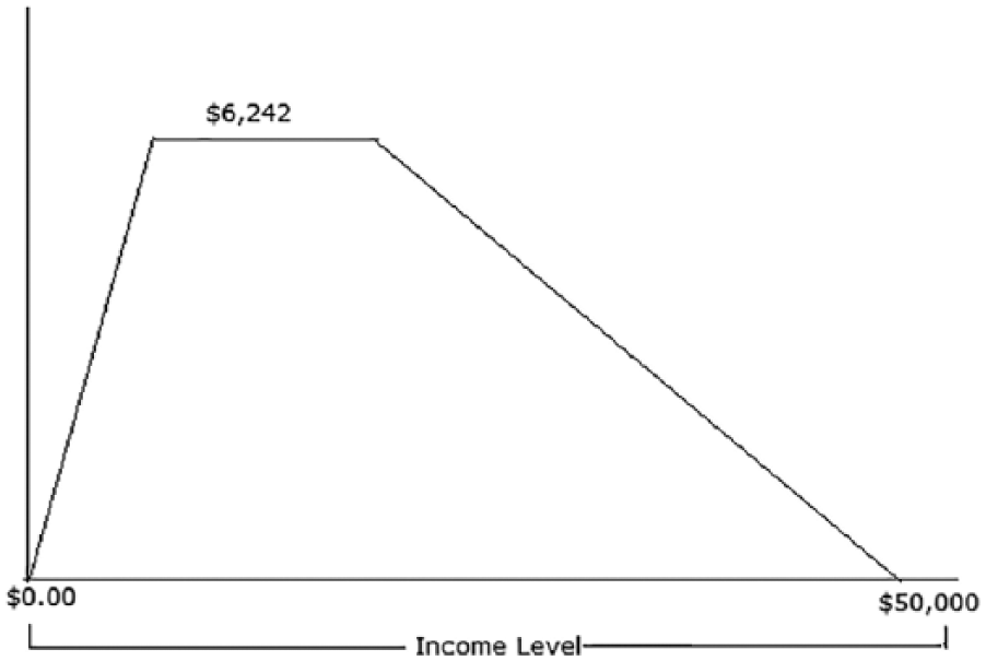
EITC diagram with phaseout and amounts (2015).
Most states piggyback on the federal EITC, using the same eligibility requirements and setting state-level credits at some fraction of the federal EITC rate. Individuals can claim both federal and state credits. State credits vary considerably. In recent years, a credit of 3.5% (Louisiana) of the federal credit is on the low end, whereas 40% (District of Columbia) of the federal credit level is on the high end (Center on Budget and Policy Priorities, 2011).
In 2012, 24 states and the District of Columbia had EITC programs. Six states have enacted the program since 2006, including Connecticut (2011), Michigan (2006), North Carolina (2007), Louisiana (2007), New Mexico (2007), and Washington (2008). 1 Three states had nonrefundable EITCs: Maine, Virginia, and Delaware (E. Williams, Johnson, & Shure, 2010). If the filer has a negative tax liability (owes less than the credit), the individual, in states with a refundable credit, receives the difference as a refundable check, while those filers who have negative tax liability but live in a state without a refundable credit do not receive the difference.
The Earned Income Tax Credit and Employment
The design of the EITC has been shown to have a significant effect on incentivizing new entrants into the workforce (Celik, 2011; Eissa & Liebman, 1996; Schmeiser, 2011; Scholz, 1996; E. Williams et al., 2010), especially among single mothers. Scholz (1996) analyzed responses to the EITC based on monthly Survey of Income Program Participation data and found that, at the national level, the EITC provided 145 million new hours of work in the labor market per year. A possible concern is that the phaseout portion could disincentivize work and thus cancel out the employment benefits. However, Scholz (1996) found that the phaseout disincentive is outweighed by the additional hours that new entrants work and by workers at the phase-in and plateau portions of the income distribution. Romich and Weisner’s (2000) ethnographic study of EITC recipients found that one third of the participants thought that the EITC had a positive linear relationship between the hours worked and the total amount of their credit, while only 2 of the 42 participants knew that they had to earn a specific amount to maximize their credits. The construction of the credit has been shown to generate positive net employment.
Schmeiser (2011) simulated the accounting and behavioral impact of a 15% expansion of the New York EITC on the state’s labor supply relying on labor supply elasticities from the literature in the range of 0.69 (Meyer & Rosenbaum, 2001) to 1.16 (Hotz & Scholz, 2001). Schmeiser estimated that between 7,125 and 21,363 single mothers would have entered the labor force based on this expansion. Despite some adverse impact of individuals leaving the labor market, this is outweighed by the 11.6 million to 34.9 million hours worked by new entrants within the labor force. In total, he found that labor earnings would also increase by $63.4 million to $94.3 million.
The Earned Income Tax Credit and Local Economic Development
The positive benefits of a state EITC program have been estimated in localized areas using input–output analyses. Low-income individuals tend to spend EITC-related tax refunds directly into the economy, while saving very little of their refunds (Berube, 2006; Romich & Weisner, 2000). In the short run, this spending has an immediate economic benefit to the local community because the multiplier effect tends to be higher (dollars are recirculated more often in the local area). This spending, according to Berube (2006), often takes the form of “(a) buying clothes for children, (b) replacing furniture and appliances, (c) repairing a vehicle, (d) going on a trip, and (e) catching up on past-due rent and utility bills” (p. 3). Berube (2006) estimated that every dollar spent on the EITC in San Antonio yielded an additional $.58 in the local economy. Similarly, a report by the Jacob France Institute (2004) estimated an employment multiplier effect of 1.41 for Baltimore City. This estimate means that for every 10 jobs that are created as a result of the direct spending of EITC dollars, 4 additional jobs will be created through indirect effects (a fraction of the salaries are respent in the local economy). For example, if the recipient buys food at a grocery store, the purchase supports the workers at the store who then spends money on other goods or services in the local economy. Input–output models can be sensitive to assumptions of the percentage of dollars spent locally.
As of 2010, a surprising 67 of the top 100 metropolitan areas are in states that did not have a state-level EITC. Tracking all forms of federal investment into urban areas, Berube (2006) found that the EITC program benefitted urban areas more than any other federal investment. Berube noted that, while many have viewed this credit as a positive for recipients, they have neglected to consider the impacts that it has on the physical location.
Theory
The most obvious indicator of interest in economic development studies is employment. The EITC has been shown to increase the employment multiplier effect at the city level; however, these effects are often estimated using static input–output analyses. As such, these are not causal estimators that directly test whether the EITC causes employment. Therefore, one cannot determine the directionality of the association or even rule out chance given the lack of confidence intervals and hypothesis testing. The question advanced then is, “Does the credit lead to a significant positive employment effect on the treatment side of the state border?” Because some of the benefit can accrue to those without the credit (due to economic leakage across the metropolitan border), the test is both more conservative and realistic. While many economic impact models, particularly input–output models, start with the assumption that the benefits will be completely localized (100% occurring in the local area), this analysis more realistically tests whether the side receiving the credit has a total economic impact that is significantly improved over the side not receiving the credit, while recognizing some of the effects of the credit may leak over to the control side. Because there is concern that these economic leakage effects could temper the generalizability of these findings, a set of robustness checks are offered that model the impacts on the entire state (where there would be a smaller potential for economic leakage) and at the metropolitan level using a synthetic control group methodology (relying on a different control group structure). Both robustness checks confirm the main findings.
There are a few possible market effects that could result from a state-level EITC, which lead to Hypotheses 1 and 2. First, given that the EITC increases the labor supply, the state-level EITC may increase the demand for local goods that result from consumer expenditures. Of course, some of this impact may be mitigated by proximity to the bordering non-EITC side, particularly for those living in one state and working in the other. Given an increase in consumer expenditures and thus an increase in the demand for labor, wages may increase, assuming no simultaneous change in the labor supply. However, the potential wage increases that might otherwise result may be mitigated by firms offering lower wages on the state-level EITC portion of the border since employees would accept lower wages in return for the credit.
The foregoing theory leads to the following two hypotheses:
Establishments, controlling for all other factors, will be attracted to the border area that offers the credit, given that individuals claim the credit on their personal income tax statements and not through a payroll tax on firms. This can affect the decision of firms to locate on the border side with the credit, as it has the potential to act as a partial wage subsidy. The theory on establishments leads to the following hypothesis:
The EITC is distributed by states to low-wage-earning residents. If a low-wage earner lives in the treatment state and works in the control state, that individual is entitled to receive the credit. If the individual lives in the control state and works in the treatment state, that individual is not entitled to receive the state credit. This makes the estimate a conservative estimate; however, it is still an appropriate test because states also want to know whether their impacts lead to improved economic outcomes relative to competing states. Furthermore, it has been determined that the EITC did not significantly affect commuting patterns from the EITC to non-EITC 1 and 2 years after the adoption of the policy. 2
Data and Method
The impacts of the EITC are not spread evenly across all industries. J. R. Williams and Kneebone (2014) and the National Council of State Legislatures (2015) noted that the five industries most affected by the EITC include accommodations and food services, construction, health care and social assistance, manufacturing, and retail trade. Furthermore, other studies use several of the same industries to study the effects of minimum wage on accommodation and food services, retail, and/or manufacturing (Card & Krueger, 1993; Rohlin, 2011), the right to work effects on manufacturing (Holmes, 1998), and the effects of sales taxes (Thompson & Rohlin, 2012).
The key dependent variables measuring economic development are derived from the U.S. Census Bureau’s County Business Patterns data (1986 to 2012). 3 These data are collected through establishment surveys on a yearly basis with consistent industry data for each sector included. From 1986 to 1997, the information relies on the Standard Industrial Classification (SIC). From 1998 to 2012, the data rely on the North American Industrial Classification System (NAICS). The variables include employment, payroll, and establishments for each county from 1986 to 2012. To account for inflation in payroll, the U.S. Bureau of Labor Statistics Consumer Price Index–Urban was used as a deflator. Payroll is adjusted to 2012 U.S. dollars for all time points.
Data for the EITC rates by state come from the Center on Budget and Policy Priorities and from the Tax Policy Center. Prior to 2000, the Center for Budget and Policy Priorities and the Tax Policy Center do not include state-level EITC rates; therefore, the data provided by the National Council of State Legislatures–Tax Credits for Working Families are used. Thus, the analyses use state-level EITC rates rather than actual dollar values of the credit. 4
The state minimum wage must be considered when evaluating the effect of the state-level EITC, given that it affects the same economic indicators for several of the same industries (Card & Krueger, 1993; Dube et al., 2010; Rohlin, 2011). Dube et al. (2010) and Rohlin established that the minimum wage rate changes across many of the same states in this study and during the same period as this study (1986-2012). The U.S. Department of Labor maintains the federal and state-level minimum wage information. Additionally, Murphy (2007) has shown that state-level unemployment insurance rates affect wage levels. Therefore, both the minimum wage and the unemployment insurance rates are included as important control variables.
While the metropolitan area is the primary economic unit, the density of the labor force may not evenly be distributed across state borders. Given that benefits from agglomeration, particularly urban agglomeration benefits of a larger labor pool and density may differentially accrue to one side of the border, a labor force density variable is included to account for this differential. Thus, if most of the economic activity accrues to one side of the border, then the model will control for the unequal distribution of economic activity across these multistate borders.
Demographic and socioeconomic data are available at the county level on a yearly basis through the Decennial Census, the Population Division of the U.S. Census Bureau, and the American Community Survey. The Population Division of the U.S. Census Bureau estimates intercensal population for the years 1986 to 1989, 1991 to 1999, and 2001 to 2004 for each of the variables included here, except for educational attainment and Hispanic population prior to 1990. 5
Table 1 provides the source, variable type, level, and year of each data source.
List of Variables to Estimate Economic Impact of State-Level EITC.
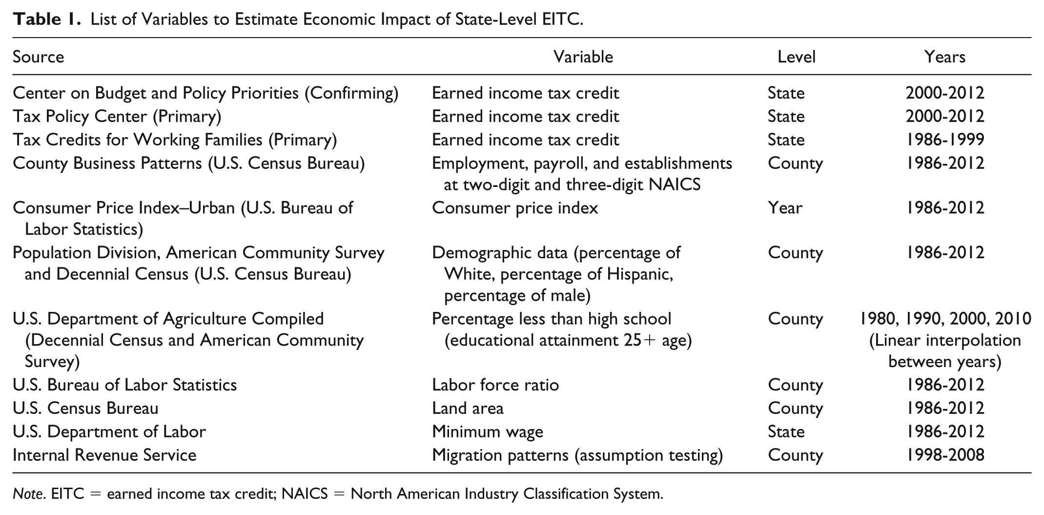
Note. EITC = earned income tax credit; NAICS = North American Industry Classification System.
Sample Design
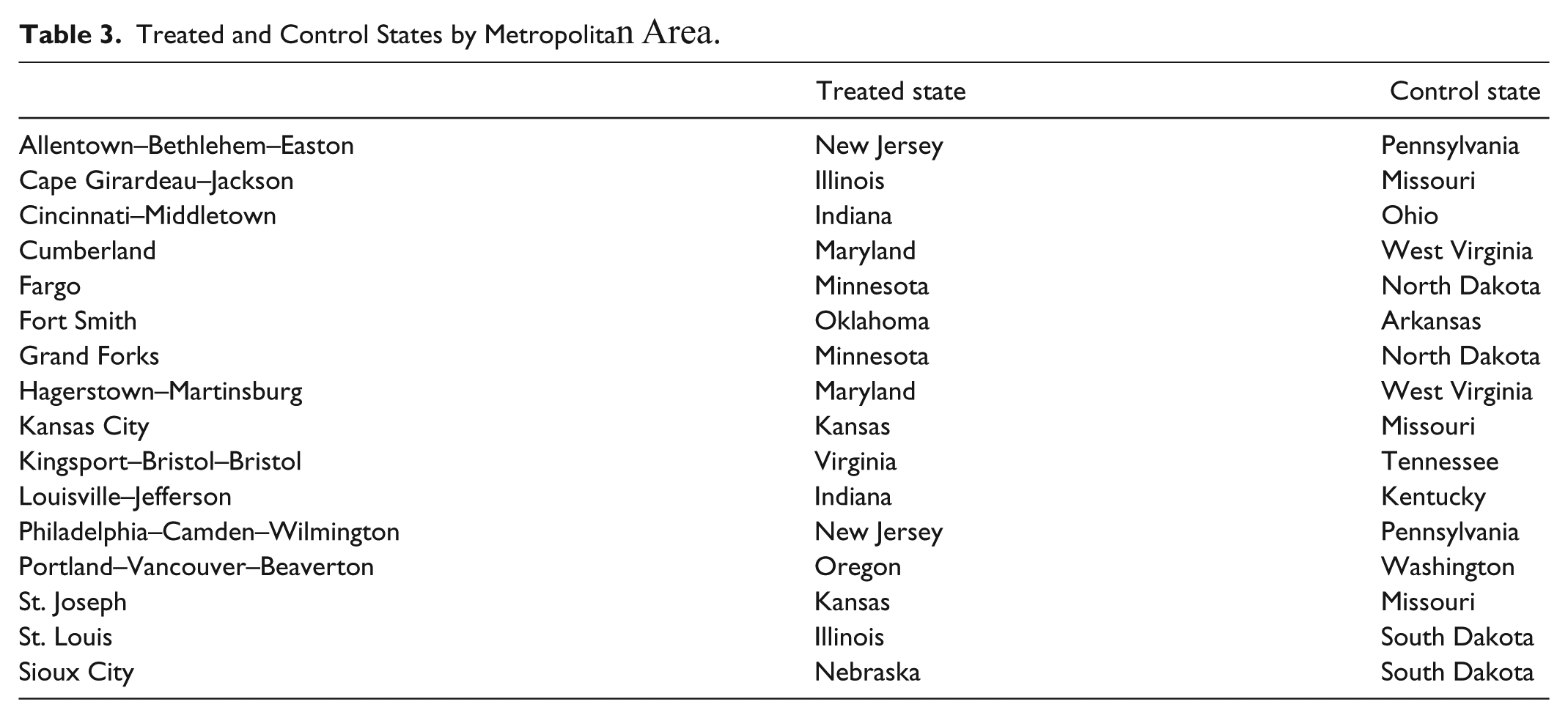
The construction of the sample started with the identification of all metropolitan areas that spanned more than one state where one state adopted the EITC between 1986 and 2012 and the other did not. This resulted in 15 metropolitan areas with a treatment and control border area over the 26-year time frame. The treatment states are included in Table 2 along with the year of EITC enactment, initial state-EITC rate (percentage of the federal credit), and the most recent EITC rate in the sample (2012). Table 3 provides a listing of metropolitan areas by treatment and control state. Table 4 compares all states on the EITC rate by year.
State-Level Earned Income Tax Credits in Sample With Year of Implementation.
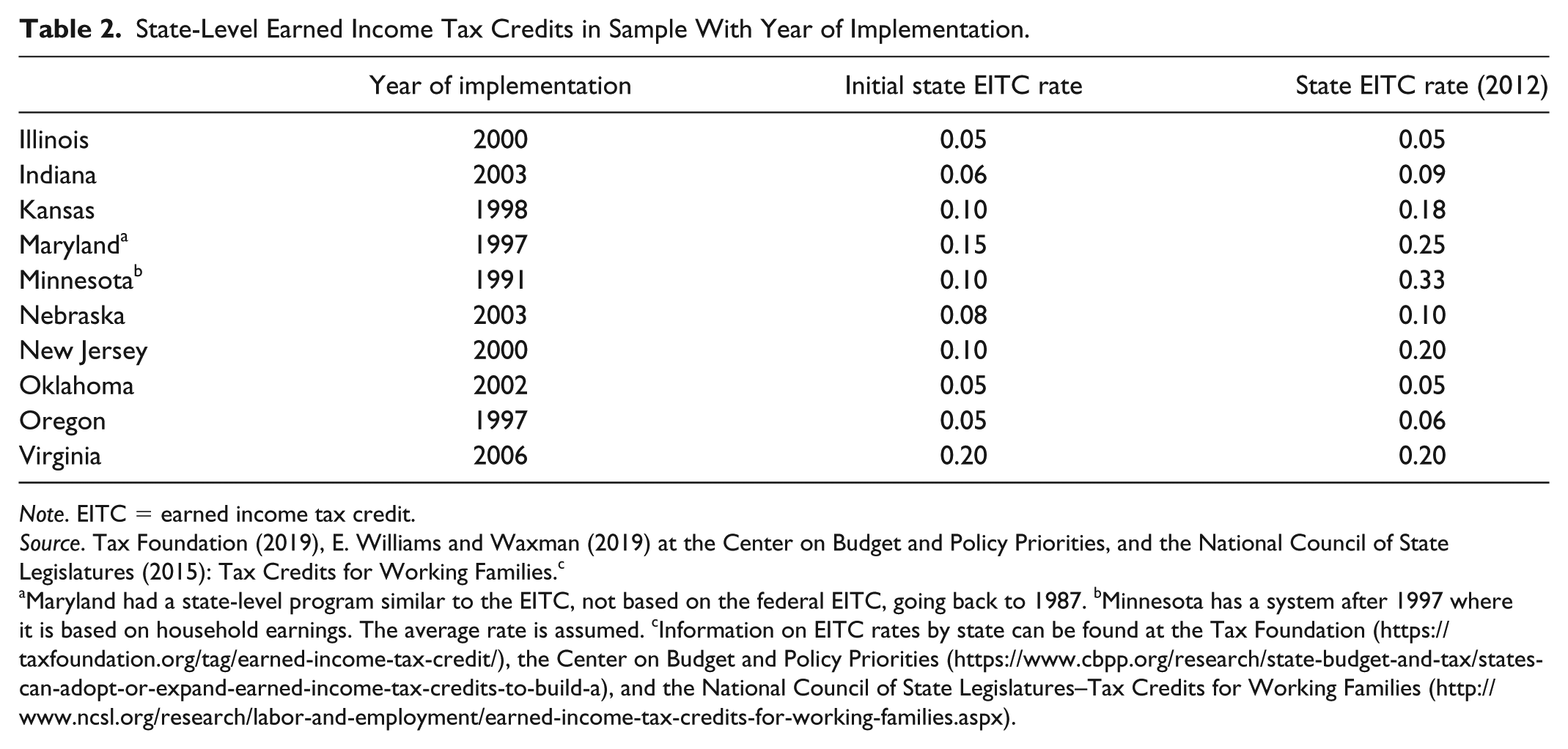
Note. EITC = earned income tax credit.
Source. Tax Foundation (2019), E. Williams and Waxman (2019) at the Center on Budget and Policy Priorities, and the National Council of State Legislatures (2015): Tax Credits for Working Families.c
Maryland had a state-level program similar to the EITC, not based on the federal EITC, going back to 1987. bMinnesota has a system after 1997 where it is based on household earnings. The average rate is assumed. cInformation on EITC rates by state can be found at the Tax Foundation (https://taxfoundation.org/tag/earned-income-tax-credit/), the Center on Budget and Policy Priorities (https://www.cbpp.org/research/state-budget-and-tax/states-can-adopt-or-expand-earned-income-tax-credits-to-build-a), and the National Council of State Legislatures–Tax Credits for Working Families (http://www.ncsl.org/research/labor-and-employment/earned-income-tax-credits-for-working-families.aspx).
Treated and Control States by Metropolitan Area.
Earned Income Tax Credit Rate by State and by Year.
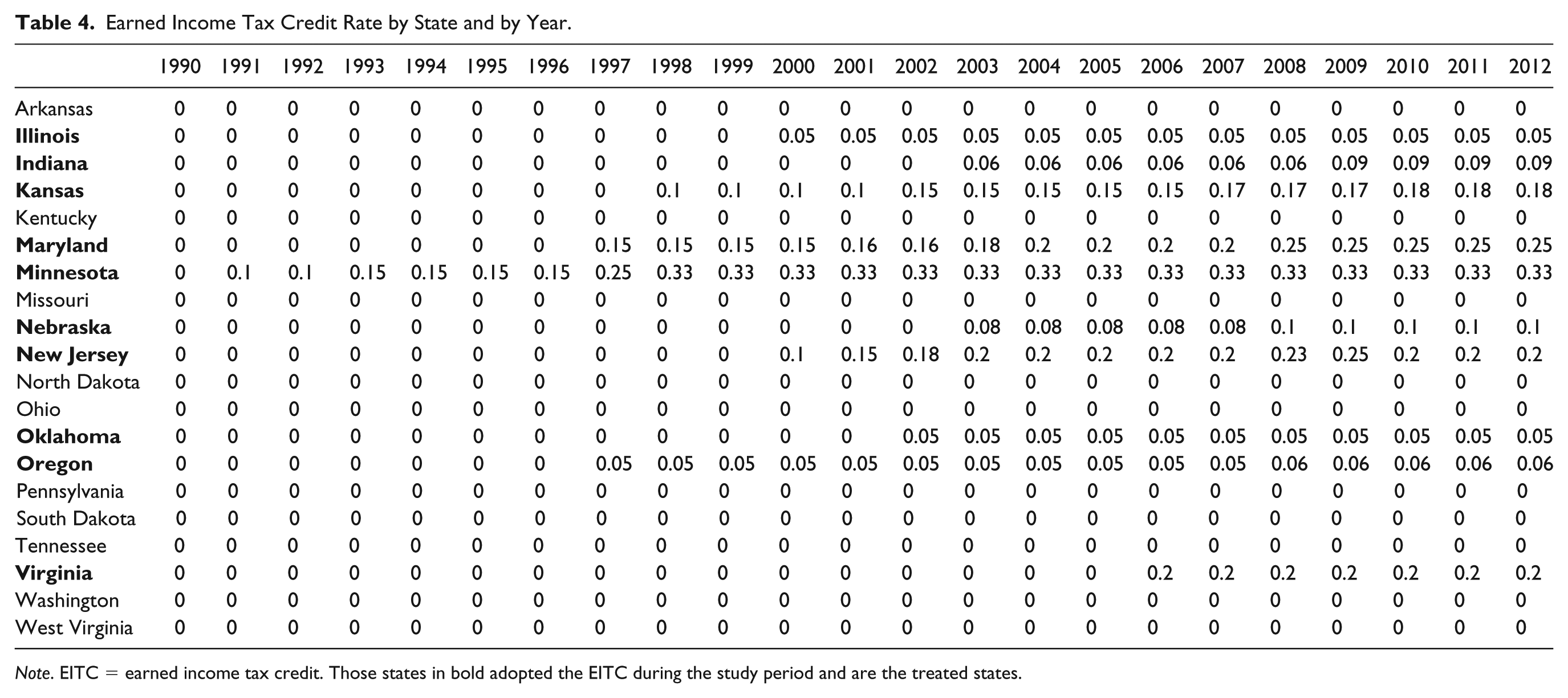
Note. EITC = earned income tax credit. Those states in bold adopted the EITC during the study period and are the treated states.
Having identified metropolitan areas in these states, counties in each metropolitan area were aggregated to construct two “border areas,” one of which contained the treated (With EITC) counties and the other contained the comparison (Without EITC) counties. 6
Variables that vary at the state level only (EITC, minimum wage rate, and unemployment insurance rate) use the state rates. The remaining variables (percentage of White, percentage of Hispanic, percentage of male, percentage with less than a high school degree, and labor force density) are aggregated across counties within each state along the border to construct the “border area.” 7
Method
To analyze the impact of the EITC on employment, wages, and establishments, this study employs difference-in-differences and triple-difference models. It also provides two sensitivity checks by expanding the difference-in-differences analyses to the state level, and a synthetic control method is applied to bolster the confidence of the findings. The difference-in-differences design at the border area level naturally controls for differences inherent across geographies (e.g., climate and regional differences) and factors unique to each metropolitan area (e.g., labor market pool and common transportation infrastructure). One benefit of the border approach, with difference-in-differences estimators, as Rohlin (2011) noted, in his study of the minimum wage, is that it “minimizes the possibility of unobserved area-specific attributes biasing the estimated effect” (p. 108). Lemieux and Milligan (2008) and St. Clair and Cook (2015) noted that comparison groups perform well as counterfactuals when they are in the same labor market as the treatment group. This methodology is further strengthened by having data over a long period of time (1986-2012). These panel data allow for time fixed effects to account for any changes that occur at the state or national level that affect local economic indicators, and unit fixed effects that account for time-invariant factors that affect economic growth. 8
An important assumption in the difference-in-differences framework is that there are parallel trends in the dependent variables before the adoption of the EITC, which is tested. A failure to find parallel trends may suggest that the supposed effect of the EITC on the outcome variables is not actually due to the credit itself but due to changes that were already underway. Additionally, since the state is responsible for adopting—and the unit of analysis is the constructed border—then the state would have to be responsive to changes in the economic structure at the border of these metros for it to present issues of endogeneity. As noted earlier, it is assumed that the state is not making decisions regarding the adoption of the EITC based on the economic circumstances of its border counties. If it was, then this may also be reflected in possible changes in these outcome variables pre-EITC and post-EITC adoption. Figures 2 through 4 provide a visual inspection of these assumptions. These figures provide confidence that the parallel trends assumption holds. The responsiveness question cannot be directly empirically tested with these data, but again it seems unlikely that states would make this policy decision based on the economic forces in several counties at the border of their state. 9
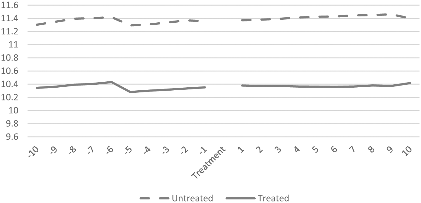
Parallel trends: Log employment (all industries).
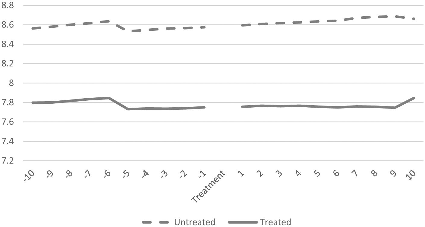
Parallel trends: Log pay (all industries).
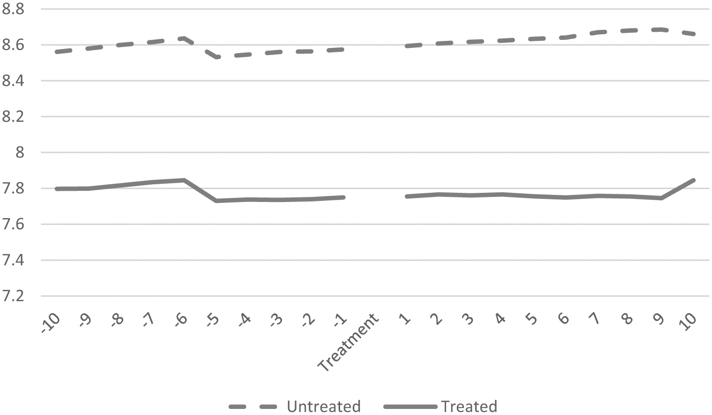
Parallel trends: Log establishments (all industries).
Table 5 provides the summary statistics for each variable used in the analyses. It would generally be expected that the observation count should be an even number with one treated observation matched to every untreated observation. This does not occur in the sample because several subindustries are not reported within each county in the sample or data are suppressed because individual establishments could be identified. Thus, many observations were missing subindustry data on car wash establishments and drinking places. Nonetheless, both sides had data on the main industries (All Sectors, Manufacturing, Construction, and Retail Trade). The dependent variables (employment, payroll, and establishments) are logged in each model. Because some of the subsectors have zero employment, this will lead to observations being dropped; however, the level of skew with these variables makes this a preferable form for the dependent variable. 10
Summary Statistics.
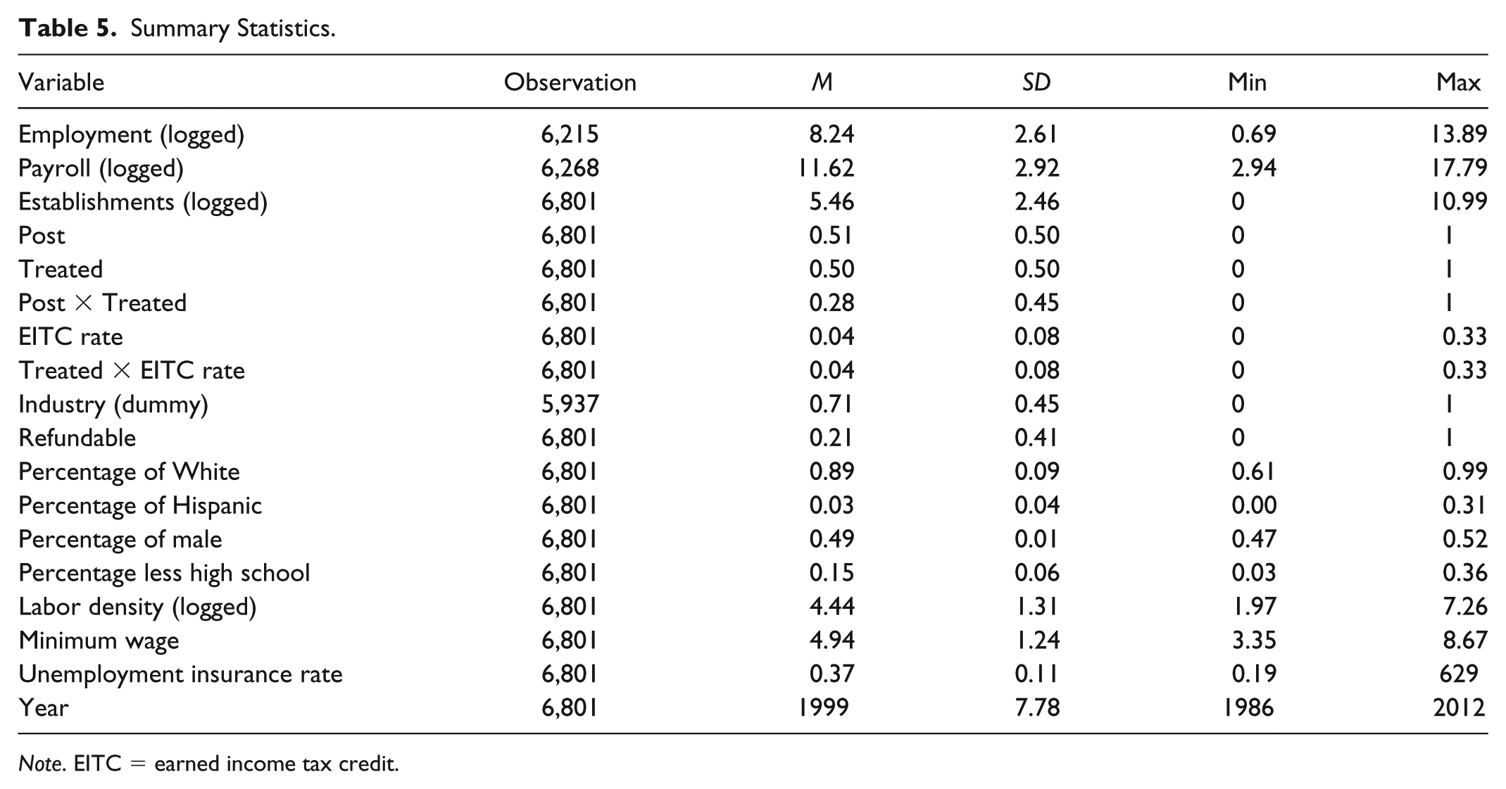
Note. EITC = earned income tax credit.
An industry dummy variable is used in several of the specifications. This is equal to one for the sectors that have been shown to be most affected or are hypothesized to be positively affected by the EITC (manufacturing, construction, drinking places, and retail trade) and equal to zero for those believed to not be significantly affected by the EITC (legal services and all other sectors).
Several states allow the recipient to receive a refundable credit, which effectively gives the recipient the difference between their tax liability and the amount of the credit. If the difference is negative, they are issued a check in this amount. Therefore, it is hypothesized that these states may experience a greater economic benefit from the credit.
The socioeconomic controls are reported as percentages at the border area level. Thus, as border areas are aggregated across counties, the number of White individuals is summed across counties and divided by the total population across counties to derive the percentage. The averages are largely in line with expectations for the period of 1986 to 2012. Several values seem to be extreme along the range. The percentage of White at a rate of 0.99 was found in the Cincinnati metropolitan area when Franklin, IN and Dearborn, IN were included. This rate, as of 2012, is now slightly below 0.98; however, before 2000, it was at 0.99. The Hispanic population has reached 0.31 in the Sioux City treated border area, with Dakota, NE, and Dixon, NE yielding a rate above 0.30 since 2010.
Labor density is included as a control variable, which is the labor force divided by the amount of total land. This variable is logged, but in level form the average for this variable is 0.08 with a range of 0.003 to 0.55. On the low end, the Sioux City untreated side has a labor density of 7.15 with a labor force of 3,340 in 1990 and 467.1 square miles of land. On the high end, the untreated side of the Philadelphia metropolitan area has a labor force density of 1,418.9 with a labor force of 1,319,420 and a total land area of 929.89 square miles. This variable controls for the potential impact resulting from agglomeration benefits accruing to one side of the metropolitan border. 11
Models
To assess the effectiveness of the EITC on economic indicators, the most basic setup for the difference-in-differences model would use a reduced-form equation such as the following:
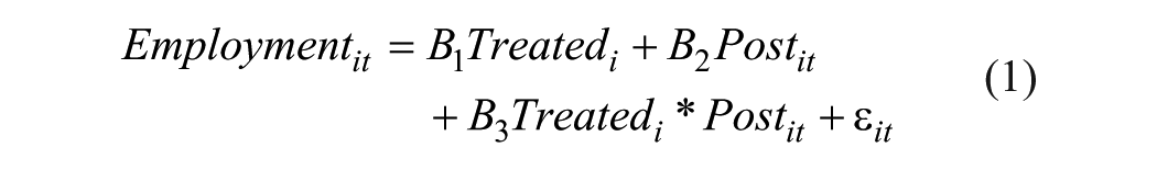
where employment is the natural log of employment in border area i, at time t (in years). Treated is an indicator variable where the treatment side of the metropolitan border is equal to one and the nontreated border area is equal to zero at all time points. Post is an indicator variable equal to one for those years after the enactment of the EITC on both the treated and untreated sides of the border.
Equation 2, therefore, addresses issues of omitted variable bias by adding a set of economic and socioeconomic control variables that also influence employment and may be associated with the use of the EITC. One important control variable is the minimum wage, which also varies across states and affects many of the same industries as the EITC. A second problem is that there is unobserved border area heterogeneity. Thus, Equation 2 accounts for this by including metropolitan border area and time fixed effects. 12
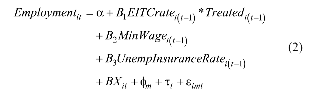
In these models, i indexes the border area that may be treated or untreated, m indexes the entire metropolitan border area, and t indexes time. X is a set of covariates serving as economic (e.g., unemployment insurance and labor force ratio) and socioeconomic controls (e.g., percentage of White, percentage of Hispanic, percentage of male, and percentage with less than a high school education). Furthermore,
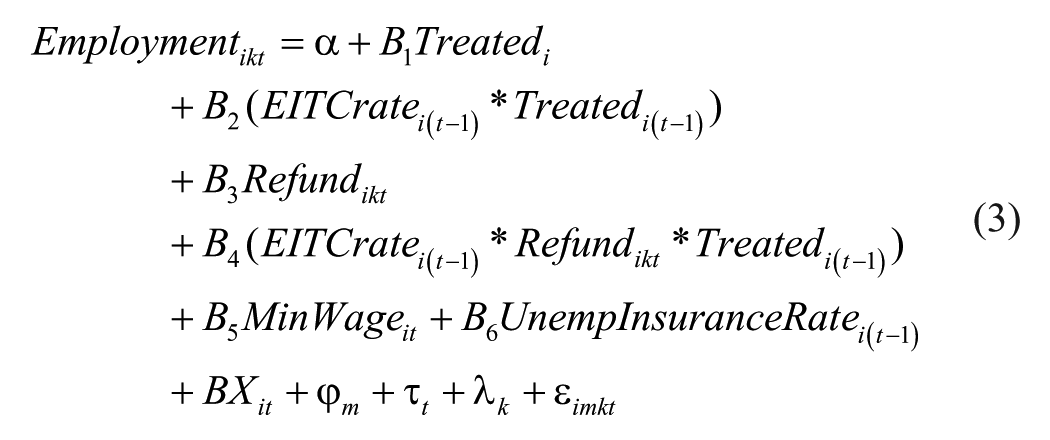
Model 3 treats the refundability (k indexes refundability) of the EITC as a third difference given that the impact of the EITC on employment should differ based on whether the credit is refundable. When the credit is refundable, the recipients receive the difference in the form of a refund check. This provides the recipients with additional resources that can be spent directly into the economy through indirect and induced spending.
Several additional models of the same form as estimating Equation 2, but with subindustry-level information (e.g., car wash industry, manufacturing, and legal services), are included to further refine our knowledge about the impact within certain subindustries.
Results
Overall, the models provide compelling evidence that the EITC does not have a significant impact on the economic indicators of interest. 15 Model 1 estimates the impact of the EITC, without accounting for the respective rate (Table 6). Model 2 is perceived to be an improvement since it accounts for the differences in state EITC rates.
Effect of EITC Treatment on Economic Indicators (All Industries).
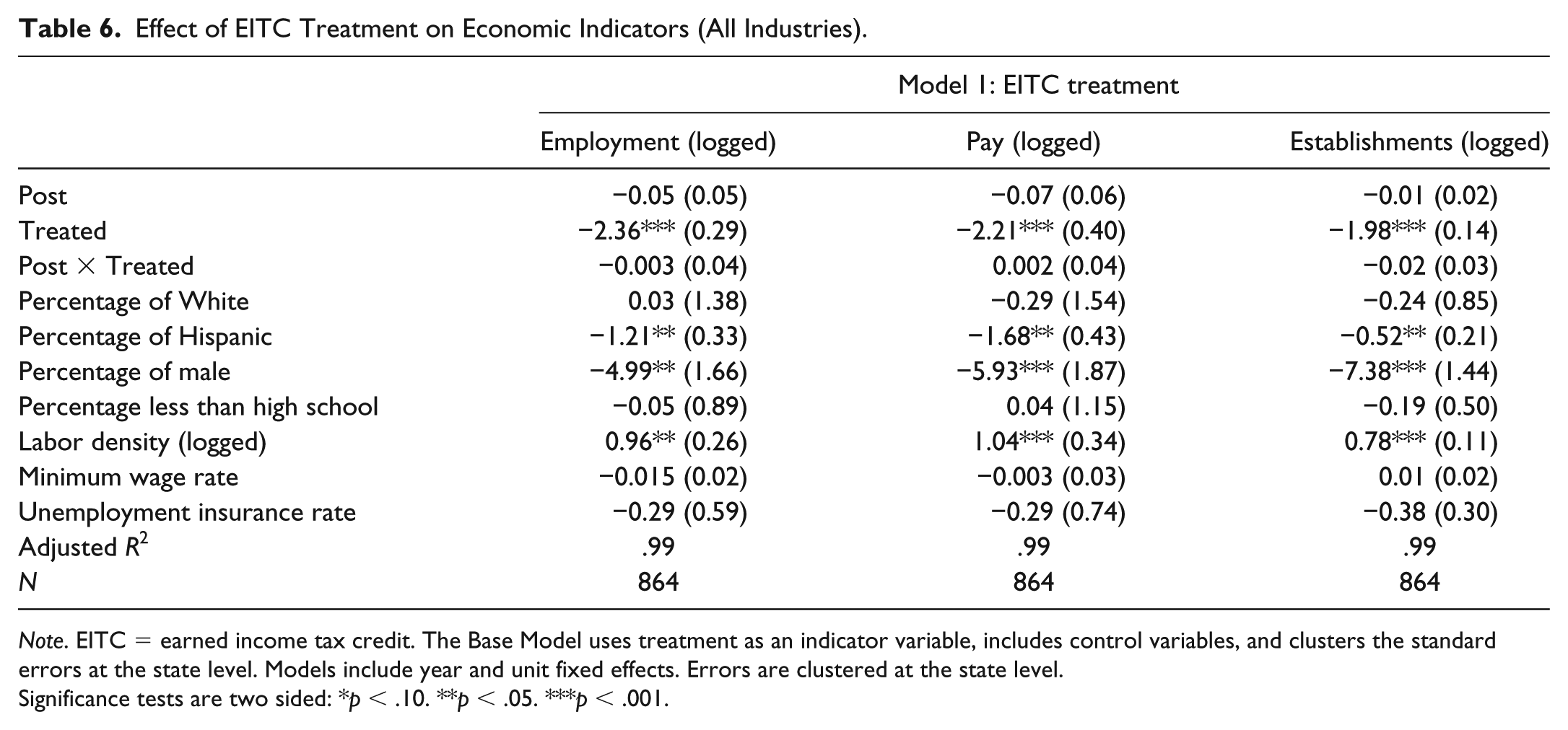
Note. EITC = earned income tax credit. The Base Model uses treatment as an indicator variable, includes control variables, and clusters the standard errors at the state level. Models include year and unit fixed effects. Errors are clustered at the state level.
Significance tests are two sided: *p < .10. **p < .05. ***p < .001.
Model 2 (Table 7) estimates the impact of the EITC on each of the dependent variables. It includes metropolitan border area and time fixed effects, control variables, and lagged effects of other policies that could affect the same outcome variables if bundled together (minimum wage and the unemployment insurance rate). It is clear that the EITC does not have a significant effect on each of the local economic indicators. 16
Effect of EITC Rate on Economic Indicators (All Industries).
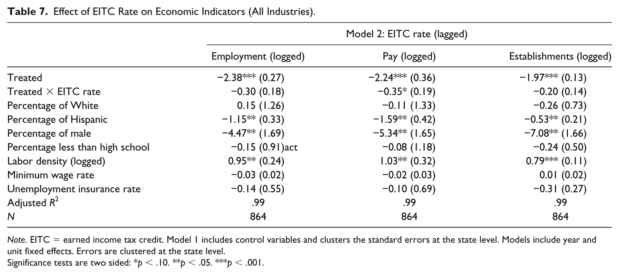
Note. EITC = earned income tax credit. Model 1 includes control variables and clusters the standard errors at the state level. Models include year and unit fixed effects. Errors are clustered at the state level.
Significance tests are two sided: *p < .10. **p < .05. ***p < .001.
Model 3 (Table 8) estimates the impact of the EITC on the local economic indicators using a triple-difference model. This refines the counterfactual trend assumptions from the more simplistic growth of the indicator variables between the treated and control group to the growth by another factor (e.g., refundable credits). The idea is that the refundable credit will provide recipients with disposable cash, assuming they have a negative tax liability, which can be spent within the economy. Despite this, the triple-difference model demonstrates the lack of a significant effect on each of the local economic indicators (employment, wages, and establishments).
Triple Differences (Refundable vs. Nonrefundable Credit) Effect of EITC Dosage on Economic Indicators All Industries.
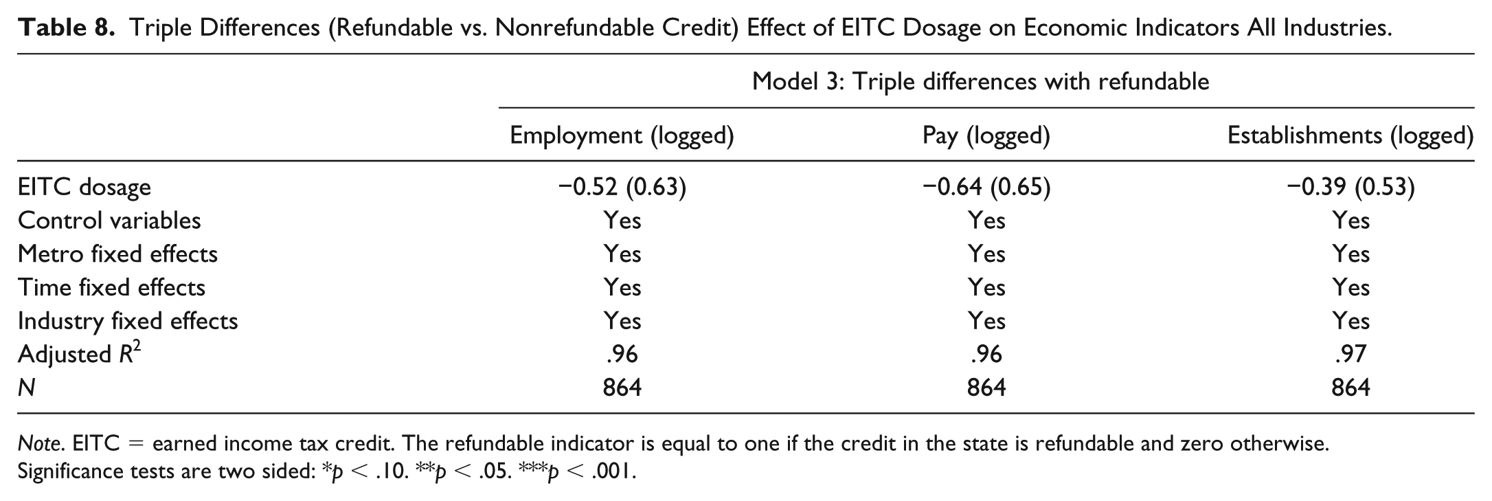
Note. EITC = earned income tax credit. The refundable indicator is equal to one if the credit in the state is refundable and zero otherwise.
Significance tests are two sided: *p < .10. **p < .05. ***p < .001.
Industry-level results allow for a refined test of the treatment effect since a differential impact is possible given that there may be a higher concentration of low-income employees working and spending money in certain industries. Testing the EITC rate impact on industries and subindustries offers more fine-grained levels of analyses if the industries are too aggregated to experience the impact of the EITC (car washes, drinking places, and legal services). Each of these models include metropolitan border area fixed effects, time fixed effects, and robust clustered standard errors at the state level. Additionally, each model includes the full set of control variables (minimum wage, percentage of White, percentage of male, percentage of Hispanic, percentage with less than a high school degree, and labor force density).
The results across the industry and subindustry models (Tables 8 through 10) show mostly no effects of the EITC on employment, payroll, and establishments. Legal service employment (−0.87%) and payroll (−1.32%) are significantly and negatively associated with an increase in the EITC. Thus, a 1 percentage point increase in the EITC at the state level is associated with a 0.87% decrease in employment and a 1.32% decrease in payroll within this sector. Further research would need to address the causal mechanism that results in this decline. Speculation may suggest that those areas benefiting from the credit have fewer demands or needs to render legal services among low-income individuals. This study provides a framework for thinking about these subindustry effects, but further research could explore the differentials across industries and subindustries. One other possible reason is that to the extent that recipients of the EITC are more likely to go to payday lenders, and thus less likely to rely on traditional tax preparation services, for which there is reason to believe this is the case, this substitution may lead to a decrease in the legal services subsector. However, this idea should be accepted with caution because even in the absence of a state-level credit, low-income individuals are still able to claim the federal credit. Any differential then between states with and without the credit should be marginal on this substitution (Table 11). As a final robustness check, these models were employed at the state level where the EITC rate did not have a significant effect on the legal service industry. 17
Difference-in-Differences by Industry With EITC Rate (Logged Employment).
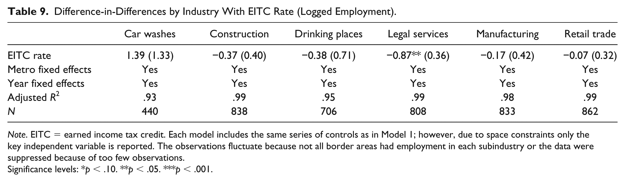
Note. EITC = earned income tax credit. Each model includes the same series of controls as in Model 1; however, due to space constraints only the key independent variable is reported. The observations fluctuate because not all border areas had employment in each subindustry or the data were suppressed because of too few observations.
Significance levels: *p < .10. **p < .05. ***p < .001.
Difference-in-Differences by Industry With EITC Rate (Logged Pay).
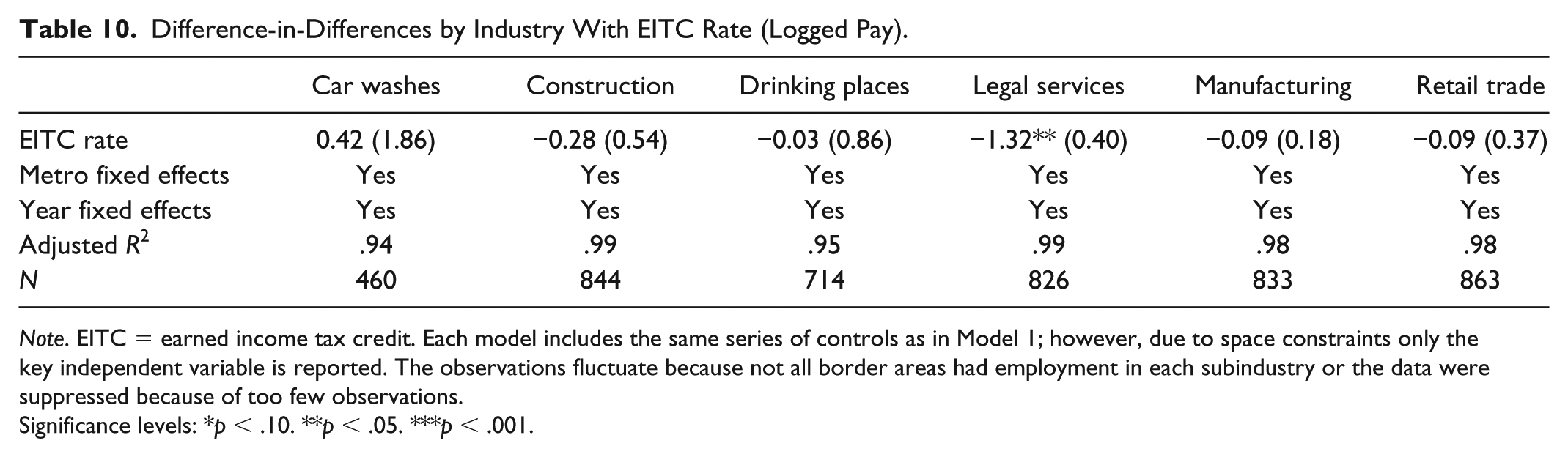
Note. EITC = earned income tax credit. Each model includes the same series of controls as in Model 1; however, due to space constraints only the key independent variable is reported. The observations fluctuate because not all border areas had employment in each subindustry or the data were suppressed because of too few observations.
Significance levels: *p < .10. **p < .05. ***p < .001.
Difference-in-Differences by Industry With EITC Rate (Logged Establishments).
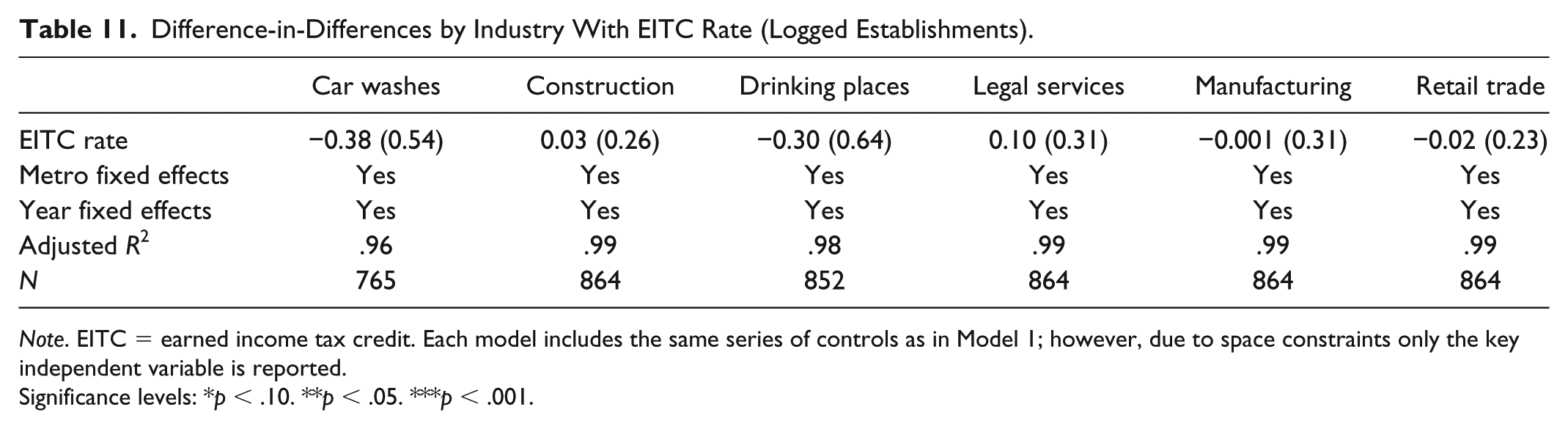
Note. EITC = earned income tax credit. Each model includes the same series of controls as in Model 1; however, due to space constraints only the key independent variable is reported.
Significance levels: *p < .10. **p < .05. ***p < .001.
Robustness Checks
While one of the core advantages of the research design is that many factors common to the metropolitan area are naturally controlled, it does create a possible concern that the parameter of interest in each case is arbitrarily deflated because of economic leakage (spillover effects). To address this concern, two additional models were utilized that would not suffer from this possibility.
The first was to conduct the same analyses at the state level, given that spillover effects at the state level, rather than across a metropolitan border, would be negligible. The results confirmed the same null findings. 18 Of course this robustness check may violate other assumptions of the difference-in-differences strategy, namely that states may adopt the credit due to economic factors within the state. This is likely less of a concern, as noted, for border counties within their metropolitan areas because states will be more concerned about state-level economic indicators.
The second robustness check used the synthetic control method (Abadie, Diamond, & Hainmueller, 2010; Abadie, & Gardeazabal, 2003). This methodology has become increasingly popular because, rather than relying on a single researcher-chosen control unit in a generalized difference-in-differences framework, which may or may not be similar to the treatment unit, it utilizes a “donor pool” of control units and weights each unit to provide a better match for the treatment unit based on preintervention trends. 19 In this study, I estimated a separate analysis for each treated unit on employment indicators across all industries. The analysis relied on all possible configurations of the control units as the synthetic control, but the algorithm optimized the set of control units that were best. The results of the synthetic control method, while not providing t tests, tend to confirm the primary findings of no significant effect of the EITC on local economic growth. Figures 5 and 6 are generally reflective of the trends across metropolitan areas. Many saw an increase in their logged employment before treatment in both the treatment and control units, but there appears to be no major change following enactment in the short or longer term. What matters more than the difference in levels is the pretrends and posttrends.
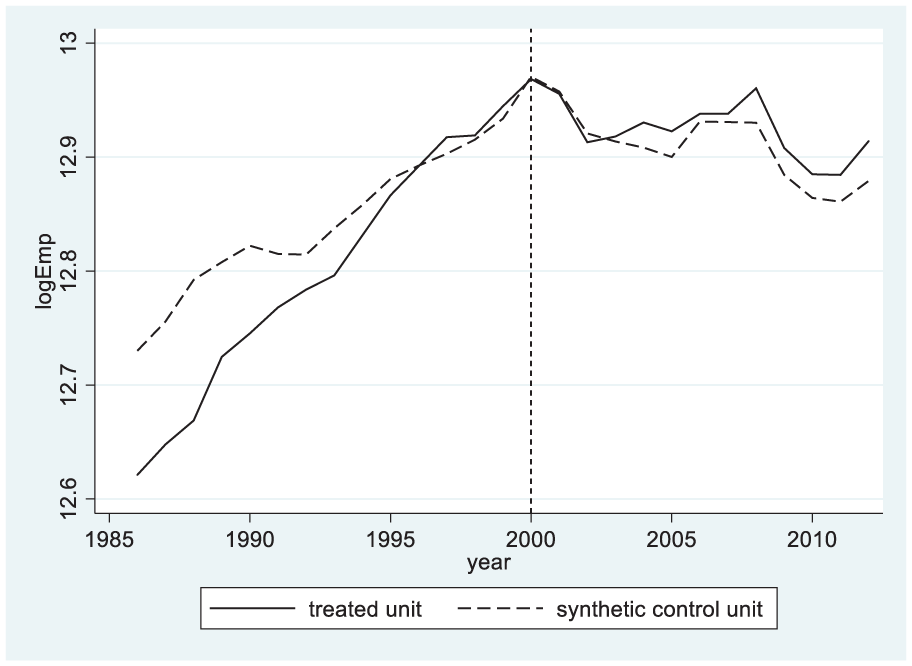
Synthetic control method for counterfactual for employment: Allentown Metro.
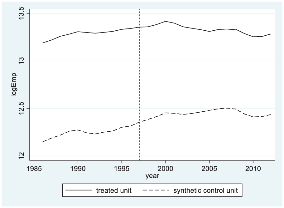
Synthetic control method for counterfactual of employment effects: Cumberland.
Conclusion
This study reveals, using a series of difference-in-differences and triple-difference estimators, that counter to expectations, the EITC showed no statistically significant impact on local economic indicators (employment, wages, and establishments) in general and across specific industries and subindustries that were thought to be influenced. Other industries may, however, experience differential effects due to a disproportionate share of recipients within industries, and based on recipient spending behavior. A strong word of caution about the program must be noted. Employment, average wages, and establishment outcomes are not the goals of the program, and therefore this should not be considered a program failure of the state EITC programs.
There are a few plausible explanations for why this research has shown mostly insignificant impacts. While impacts may be found at more granular geographical levels or within subindustries, states enact policies to address state-level concerns. While selecting border counties within metropolitan areas has the benefit of controlling for factors associated with the metropolitan area, overall positive benefits may still accrue to the state in the form of addressing economic or equity concerns.
The choice of restricting to border areas was intentional to identify the local economic impacts that resulted from the credit. As this was the motivating question (focused on urban areas generally), this selection was most appropriate. However, expanding to a county-level analysis using the entire border between two states would provide additional statistical power. The drawback of doing so is that labor market sharing between counties may no longer be naturally controlled for by the research design.
The main results held across specifications of the model and across robustness checks that utilized state-level economic indicators and a synthetic control method developed by Abadie and Gardeazabal (2003) and Abadie et al. (2010).
Despite the null findings of this research, political decision makers should continue to realize that the goal of the EITC is not simply about the local economic effects. Rather, the EITC is primarily a tool to alleviate poverty (Eissa & Hoynes, 2006) and to counteract the regressive effects of rising payroll taxes (Crandall-Hollick, 2011). The effect of this policy to do so, as shown in the literature review, is well-documented and broadly supported. Indeed, a very plausible reason why effects were not found is that the size of the credits themselves may not be large enough to affect the local economy. In the case of Illinois, 5% of the federal EITC in a single-person household may realize a credit worth only $18. If the goal of these programs were to become tools to bolster the local economy, then the credits may need to be larger to move the needle on total employment, wages, and the number of establishments.
Footnotes
Declaration of Conflicting Interests
The author declared no potential conflicts of interest with respect to the research, authorship, and/or publication of this article.
Funding
The author received no financial support for the research, authorship, and/or publication of this article.