A Scalable Energy–Economy Model for State-Level Policy Analysis Applied to a Demand-Side Management Program

Abstract

Over the past two decades, states and cities implemented low-carbon energy development, renewable portfolio standards, demand-side management (DSM), renewable energy production incentives, green building requirements, regional carbon trading agreements, and other energy-based economic development initiatives. Yet the dearth of state-level and substate-level models makes it difficult to predict the effects of such actions. This article addresses this shortcoming by presenting the performance results of the new Indiana Scalable Economy and Energy Model (IN-SEEM)—a model utilizing a dynamic, simultaneous equations framework—and demonstrates the model’s capabilities with an analysis of electricity price increases from a DSM program in the state of Indiana. Overall performance of the model is strong, with high adjusted R² values and low mean absolute percent errors for most of 30 endogenous variables. A DSM price increase analysis finds variation in impact across the state’s 10 major economic sectors and small changes in energy consumption.

Keywords

state-level modeling energy policy energy-based economic development demand side management (DSM)electricity prices

Energy and environmental policies at all levels of government, as well as energy-based economic development (EBED) activities, have important but often poorly understood economic consequences, particularly at the state and local levels. Lawmakers and economic development entities at such levels often base their decision making about EBED or environmental policies on preconceptions about the economic effects of proposed projects or policy changes. For example, during the congressional climate change legislation debates spanning 2007 to 2010, interest groups in the Midwest were concerned about the negative impact that proposed caps on emissions might have on state and regional economies. At the same time, others forecasted a surge in job growth due to the development of new approaches to energy technology and the emergence of new industries to support “greener” energy. Lawmakers involved in this debate in Congress faced a lack of reliable information regarding the potential effects of their decisions on the very constituents they were trying to represent.

Part of this confusion stems from difficulties in modeling the effects of energy policies and EBED at a subnational level. At the same time, state and local governments have been the primary drivers of energy and climate policy in the United States over the past two decades in the absence of firm commitments by the federal government. States and cities have designed innovative policies for low-carbon energy development, such as renewable energy portfolio standards, renewable energy production incentives, energy efficiency incentives, technology zones, sustainability incentives, and even regional carbon trading agreements (Bushnell et al., 2007; Carley, 2011; Rabe, 2008; Wiser et al., 2000). The degree of state and local involvement in energy issues across the country suggests significant potential for energy efficiency, energy security, carbon mitigation, and economic development (Rabe, 2008; Wei et al., 2010). EBED crosses disciplines, and its pursuit of job creation and retention and wealth accumulation relies on coordination among governments, industries, policy makers, and economic development officials (Carley, 2012; Carley et al., 2011). Such complexity requires sophisticated tools for estimating the impacts of EBED. Yet analysts’ ability to predict the effects of state policies and economic development activities—or to measure whether actual outcomes resemble the theoretical potential of these policies at the subnational level—is poor (Chen et al., 2009).

Here, we present the Indiana Scalable Energy–Economy Model (IN-SEEM), an Indiana state and substate econometric model. The model offers potential advantages over other models for questions that relate to the economic effects of energy policies and economic development activities that affect energy prices at more disaggregated levels of geography. To this end, we provide a simultaneous, dynamic system of equations, a type of econometric model built around key economic variables at the state and substate levels. The objectives of IN-SEEM are twofold: to provide a better tool for evaluating the potential economic consequences of energy price changes brought about by energy policies and EBED activities in the state of Indiana and to serve as a proof of concept for the accuracy and usefulness of econometrically determined equations for energy–economy modeling at the subnational and substate levels. We first explain how subnational econometric models address an important gap in energy–economy modeling approaches, particularly as they relate to present U.S. energy and climate circumstances. We then present IN-SEEM and its performance diagnostics. We subsequently illustrate the model using a real-world demand-side management (DSM) policy scenario that is particularly relevant to Indiana’s energy policy experience as a coal-intensive state with an economy that is potentially vulnerable to energy policy disruptions, particularly as they relate to changes in energy prices.

Energy–Economy Modeling

When modeling the connections between energy and the economy, the choice of model has profound impacts on results (Jaccard et al., 2003; Rivers & Jaccard, 2005). Designers and users of models are required to address trade-offs among important characteristics. Three of these have been described in the modeling literature as (1) technology explicitness, (2) microeconomic realism, and (3) macroeconomic completeness (Hourcade et al., 2006; Jaccard, 2005). This study adds a fourth criterion: geographic specificity. Models will be most useful when they can accommodate multiple geographic scales. For state and local policy makers and economic development officials to be informed about the effects of price changes caused by energy policies or other interventions, they need analyses that effectively model economic impacts at state and substate levels.

Top-Down Versus Bottom-Up

The effort to meet the four criteria in model design highlights one of the dominant issues in energy–economy modeling over the past two decades: the relative strengths and weaknesses of so-called “bottom-up” and “top-down” models. Before discussing their merits, it is important to note that neither should be considered unconditionally better than the other; choosing one type of model over another is instead driven by the types of questions the analyst wishes to answer.

Bottom-up models refer to a class of tools based on engineering economics and technology characterizations. These models tend to be optimization models wherein prices and the demand for energy are exogenously specified and rational behavioral responses are assumed. They are technology explicit and can be used to identify possible energy system development paths under different policy constraints and energy price assumptions.

In contrast, a top-down modeling approach examines the economy as a whole, based on historic or theoretical relationships among key variables. The focus is on economy-level perturbations, in which typical outputs of interest include measures of wages, gross domestic product (GDP), employment, or personal disposable income. One limitation of top-down models is the inability to capture behavioral responses, and so such models are poorly suited to policies focused on voluntary measures. Top-down models assume the economy will continue to respond to shifts in price variables as it has in the past. Econometric models can embed a generic technological advance, such as autonomous energy efficiency improvement, but generally they do not capture technology advances that are caused by a new direction in technology development policy (Grubb et al., 2002).

To build on the respective strengths of the top-down and bottom-up models, hybrid models are designed to blend the economic modeling methods with technological representations. These models can show the effects of changes in energy prices and policies on the broader economy generally and on energy costs and technology mix in particular.

A set of commonly used energy-economy models that allow for subnational analysis is summarized in Table 1, with selected citations provided for model documentation. Models can be classified according to whether they are top-down, bottom-up, or a hybrid, and within these classes, models may use one or more modeling techniques. While many models attempt to represent subnational energy-economic systems, improvements are needed for representing technological explicitness, microeconomic realism, macroeconomic completeness, and geographic specificity.

Table 1.

Energy-Economy Models With Subnational Capabilities.

Model	Techniques	Geographic scales	Citation(s)
Bottom-up
MARKAL	Linear programming	National, state	McCollum et al., 2012; Khadka Mishra, 2009; Shakya, 2007; Lu et al., 2016
ReEDS	Linear programming	Multiple U.S. regions	Short et al., 2011
Hybrid
NEMS	Partial equilibrium, linear programming	National, 9 U.S. regions	Gabriel et al., 2001
GCAM-USA	Partial equilibrium, linear programming	State (50)	Kim et al., 2006
BEAR	CGE, technology modules	State (California)	Roland-Holst, 2011, 2010, 2008
DIEM	CGE, linear programming	14 U.S. regions	Murray et al., 2015; Ross, 2014a, 2014b; Ross, Hoppock et al., 2015; Ross, Murray et al., 2015; Ross and Murray, 2016
NewERA	CGE, linear programming	11 U.S. regions	Montgomery et al., 2014; Tuladhar et al., 2015
US-REGEN	CGE, linear programming	15 U.S. regions	Blanford et al., 2014; Electric Power Research Institute, 2014
Top-down
IMPLAN	IOA	National, state, county	Collins et al., 2012; Jones et al., 2010; Mehmood and Pelkki, 2009
JEDI	IOA	State	Considine and Manderson, 2013; Slattery et al., 2011
NDIOM	IOA	State (North Dakota)	Coon et al., 2012
ISER-AKIOM	IOA	State (Arkansas)	Goldsmith, 2000
E3ME	IOA, econometric models	Multinational (European Union)	Pollitt et al., 2015, 2017
REMI PI+	IOA, CGE, econometric models	National, state, substate	Miller et al., 2010; Rose et al., 2012, 2011; Rose and Wei, 2009
RHOMOLO	DSGE	Subnational (European Union NUTS-2)	Brandsma et al., 2015; Brandsma and Kancs, 2015
ADAGE	CGE	State	Ross, 2008; Ross et al., 2008

Note. CGE = computable general equilibrium; IOA = input–output analysis; DSGE = dynamic stochastic general equilibrium; NUTS = Nomenclature of territorial units for statistics.

Among the energy–economy models in Table 1, three come closest to addressing each of the four evaluative criteria: the Energy-Environment-Economy Model for Europe (E3ME) (Pollitt et al., 2007; Pollitt et al., 2015), REMI Policy Insight + (REMI PI+), and the Regional Holistic Model (RHOMOLO; Brandsma et al., 2015; Brandsma & Kancs, 2015). Yet even these three substantial achievements in energy–economy modeling face shortcomings. E3ME cannot disaggregate effects below the national level. REMI PI+ has the advantage of geographically specific and historical data to estimate parameter values in econometric equations; however, the REMI approach imposes exogenous model specifications not based on historical, local relationships. These equations typically exhibit low goodness-of-fit and predictive abilities (e.g., Regional Economic Models, Inc., 2007), reducing the microeconomic realism of the results. While RHOMOLO is well suited to the latter three of the evaluative criteria, macroeconomic completeness is limited by the restriction of the dynamic stochastic general equilibrium model to only six economic sectors.

The Indiana Scalable Energy–Economy Model

The selection of the appropriate modeling approach should depend on the research questions, and the motivation behind IN-SEEM explains why we chose a top-down econometric model. Our initial —and current—intent was to build a model that would (1) incorporate the energy system, (2) incorporate the economic system, and (3) be capable of performing analysis at any state or substate geography. Many existing models exclude at least one of these components. Furthermore, the questions we intend to answer with IN-SEEM relate to how energy and environmental policies can be expected to affect the broader economy through such interventions’ effects on prices. This motivation argues against a bottom-up modeling framework like MARKAL. In contrast to the CGE approach, an econometric system of equations is flexible enough to discover relationships among variables that may not be obvious at the outset and may be peculiar to the geography being studied. The nature of our underlying research questions demanded capabilities that existing models could not provide.

As this discussion highlights, there is a need for tools that can help stakeholders understand the consequences of the state’s energy choices for the state economy, energy security, and environmental impacts. We address these gaps in economic modeling capabilities through the development of a series of econometrically estimated relationships describing the state economy, with an emphasis on the connection between energy demand, energy prices, and economic activity. The methods are generalizable to other states. This work builds on and is informed by earlier modeling of the interaction of climate change, energy development policy, and Midwest economies by Rubin and Hilton (1996) and Rubin et al. (1997), but provides a more disaggregated approach and an extensive energy consumption sector.

The use of a system of simultaneous equations to build a subnational energy–economy model offers several advantages. First, by drawing on local data, this approach fulfills the goal of geographic specificity. Results of our analysis have direct relevance for local policy makers. Second, this modeling technique allows for equation specifications that are flexible enough to be particular to each energy and economic sector and responsive to the research questions of analysts. Furthermore, the equation specifications will also be particular to the geographic scope of the state for which the data are assembled: Specifications developed for the state of Indiana are not necessarily appropriate for other states or locations. This flexibility and particularity are the foundation of microeconomic realism. Third, the available data allow for a broad range of economic sectors (10) and energy markets (7), increasing macroeconomic completeness. As a top-down model, IN-SEEM is not technologically explicit in its current form, though it is compatible for linking to a bottom-up model developed for the state. That is, forecast outputs from an econometric system of equations could be used as inputs in a bottom-up model and costs estimated by a bottom-up model could be used as inputs in the system of equations.

Methodological Approach

IN-SEEM is structured in a dynamic, simultaneous framework with the end goal being a model that can help policy makers, economic development officials, and other key stakeholders assess the potential economic consequences of energy price changes brought about by energy policies or EBED. Econometric models differ from other types of models due to their ability to uncover relationships between endogenous and exogenous variables over time, and to follow those relationships in an integrated and dynamic way. We rely exclusively on time-series data and focus on relationships that are specific to the state. Other model types often use cross-sectional relationships that are fit over multiple geographic areas, yielding model structures that are averaged across diverse jurisdictions.

The simultaneous equation structure of the model is well suited to the task of evaluating how energy-related policies and economic development initiatives affect economic activity. The majority of variables appear on both the right- and left-hand side of the equations, as described in more detail below. This simultaneity better emulates the actual economic system. Economic variables, such as employment, are partially determined by many factors, such as energy prices and gross state product (GSP). The dynamic nature of the model enables economic impacts to accumulate over time through the use of lagged explanatory variables. Determining policy impacts is a matter of calculating the differences in predicted values between baseline and policy scenarios. The explicit linkage of diverse economic sectors through this structure simulates the interdependent nature of the economy. Thus, the effects of EBED activities or related policies can be transmitted throughout the model, revealing the direct and indirect impacts of a broad range of actions, as long as the policy being examined is expected to affect energy prices.

Data

The data for IN-SEEM are drawn from a variety of sources. The U.S. Bureau of Economic Analysis (BEA) provides data on employment, earnings, nonwage income, GSP, GDP, and population. The Bureau of Labor Statistics (BLS) provides data on unemployment and labor force participation and consumer price indices (CPI). Data on energy prices and consumption at the state level are available from the Energy Information Administration’s (EIA) State Energy Data System. Climatological data are available from the National Oceanic and Atmospheric Administration’s (NOAA) National Climatic Data Center. The annual data for the model span the period from 1977 to 2011. All dollar values were converted to 2011$.

Some data discontinuities required adjustments with dummy variables over the sample period. Between 2000 and 2001, the BEA reclassified economic sectors from the Standard Industrial Classification System (SIC) to the North American Industry Classification System(NAICS). The BLS’ introduction of new Current Population Survey (CPS) population controls in 1990 created a discontinuity in unemployment data. GSP values have a discontinuity in 1997 due to a classification change in that year.

To run forecasts beyond the sample period, we developed projections for exogenous inputs to the model, including national GDP growth, earnings in farming at the national level, and heating and cooling degree days. For national GDP growth and farming earnings, the projections were calculated using a stepwise autoregressive procedure. For heating and cooling degree days, “normal weather” values for heating and cooling degree days from 1981 to 2010 were used for the projected values.¹ In an ideal model (i.e., one that had both top-down and bottom-up components), energy consumption and prices could be projected based on the interaction between supply- and demand-side factors, such as assumptions about generation technology and capacity, energy suppliers and the regulatory environment in which they operate, and interstate system operations. In the absence of such completeness, we rely on forecasts from the EIA,² whose own assumptions are subsumed into our model. The Indiana Business Research Center, a research organization affiliated with Indiana University, developed forecasts of the state population and labor force participation rate.

The data collection used in IN-SEEM is a template for other jurisdictions. In general, geographic specificity and macroeconomic completeness are best served by drawing on data that are available at appropriate geographic resolutions and cover the widest array of energy markets and economic activities. For the United States, most of the data sources listed here will be appropriate. The availability of data in other jurisdictions may suggest an alternative suite of variables for model building, as with the data in Eurostat for NUTS-2 and NUTS-3. Unfortunately, theoretically important variables, such as interstate trade or sectoral output, are not available for the state of Indiana, and such data limitations reduce macroeconomic completeness and suggest fields where government agencies might focus further attention on data collection and reporting. In the absence of data on the interstate nature of, say, the electrical grid and related markets, models like IN-SEEM will be restricted in the types of policies they can model. The flexibility of econometric systems of equations, however, allow for these open system relationships to be modeled where relevant variables are available.

Model and Modeling Approach³

Table 2 identifies the variables included in the model. Standard economic indicators representing employment and earnings are used for 10 economic sectors. The econometric model provides projections for 30 dependent variables: a total of 7 energy consumption; 20 equations representing employment and earnings per employee across 10 economic sectors; and 3 state-level macroeconomic indicators: per capita GSP, the unemployment rate, and per capita nonwage income. Exogenous variables include population, climatic variables, national-level economic data, and—most important—energy prices for natural gas, motor gas, and electricity. Among the 30 main equations, explanatory variables include both exogenous and endogenous variables, resulting in a complex and dense system of equations. We provide model specifications for all 30 main equations in the appendix (available online as a supplement to this study). An examination of those equations reveals the ways IN-SEEM captures not only the intersectoral relationships between the energy sector and the broader economy but also the relationships between and among different industries. For example, employment in manufacturing (as estimated within IN-SEEM) is a function of natural gas prices for industrial end users as well as employment in the services, constructions, and transportation and utility sectors.

Table 2.

Indiana Econometric Model Endogenous and Exogenous Variables.

Employment and earnings per employee by sector
Construction	Mining
Farming	Retail trade
Finance, insurance, and real estate	Services
Government	Transportation and utilities
Manufacturing	Wholesale trade
Energy variables
Consumption	Price^a (exogenous)
Commercial electricity	Commercial electricity
Industrial electricity	Industrial electricity
Residential electricity	Residential electricity
Commercial natural gas	Commercial natural gas
Industrial natural gas	Industrial natural gas
Residential natural gas	Residential natural gas
Motor gasoline	Motor gasoline
Economic variables
Gross state product, per capita	Gross domestic product, per capita (exogenous)
State nonwage income, per capita	National nonwage income, per capita (exogenous)
State unemployment rate	National unemployment rate (exogenous)
Climate variables
Annual cooling degree days^b (exogenous)	Annual heating degree days^b (exogenous)
Dummy variables
Post-1990 dummy (exogenous)	Post-2001 dummy (exogenous)
Post-1997 dummy (exogenous)

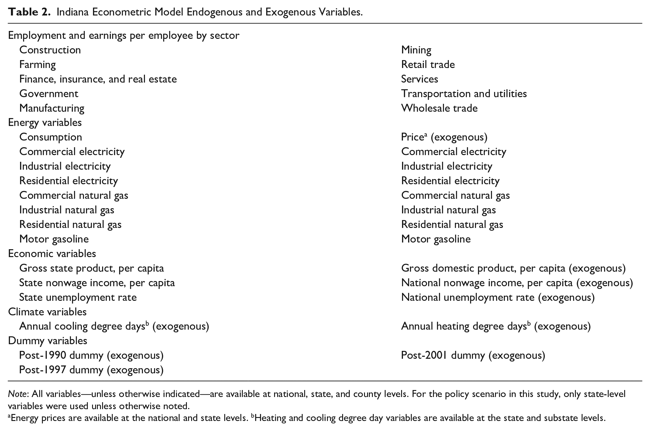
Note: All variables—unless otherwise indicated—are available at national, state, and county levels. For the policy scenario in this study, only state-level variables were used unless otherwise noted.

Energy prices are available at the national and state levels. ^bHeating and cooling degree day variables are available at the state and substate levels.

There are two goals in building econometric equations for the 30 dependent variables. First, drawing on local historical data should yield equations that are empirically sound. Second, the equation specifications should conform to theoretical expectations of relationships between the energy sector and the broader economy. The basis of microeconomic realism lies in the ability of econometric systems of equations to fulfill both goals during model construction and calibration.

In choosing and estimating econometric equations, one must seek to satisfy several empirical criteria to avoid statistical pitfalls. First, goodness of fit can be measured by a high adjusted R² for each equation and significant p values for all variables of interest. Second, equations should not suffer from common problems like autocorrelation or near perfect multicollinearity. In almost every equation, the tolerance values in IN-SEEM indicate no multicollinearity. However, collinearity is not a threat to the robustness of a predictive model, so long as it may be assumed that the relationship between two collinear explanatory variables does not change over time; where we did observe low tolerance values, this assumption was plausible. Third, the overall system of equations should be exactly or overidentified and satisfy the rank and order conditions. Fourth, the linkages between dependent variables within the system of equations should establish stable forecasts over time. Fifth, the model should produce predictions for each dependent variable over the sample period that deviate as little as possible from the actual observations, as measured by the mean absolute percent error (MAPE) for each data series. Ignoring or failing to maximize these metrics would result in a model with poor analytic capacity.

While these requirements are stringent, the construction of the econometric equations includes considerable latitude in the model specification process. This flexibility springs from the fact that, for each dependent variable, one might find several possible specifications that meet the criteria listed above. Unlike causal modeling, there is no unique model specification for each equation; rather, exploring associations among the data can reveal many mechanisms by which energy and the economy may interact. The set of possible equations must be narrowed to only those that are theoretically sound. Primarily, there must be some obvious—or at least plausible—mechanism by which each explanatory variable is associated with the dependent variable. We allow for lags among the explanatory variables, so long as these can be theoretically justified. Second, the parameter estimate on each explanatory variable should be in the expected direction. For example, energy consumption can be explained by negative own-price elasticity and positive cross-price elasticity. There may remain many specifications that meet the requirements of theory and empirics, each emphasizing different relationships among the variables. Modelers thus have the flexibility to select specifications most appropriate for different research questions. In this article, we have used the most plausible and empirically robust specifications in our final system of equations.

Most of the standard assumptions of the general linear model apply to all equations. Statistical theory, however, leads us to note that the assumption of no relationship between the independent variables is violated in any stochastic equation that includes an endogenous variable on the right side. While simultaneity bias can be corrected with two-stage least squares (TSLS) estimation, previous research on regional econometric models and substate level data has demonstrated that TSLS—or any simultaneous equation estimation technique other than ordinary least squares (OLS)—actually results in less accurate sample period simulations and minor impacts on the parameter estimates (Solomon & Rubin, 1997). This is due to data errors and sampling bias in regional data; hence, initial estimation of the model’s equations was carried out through OLS.

Applying the Econometric Systems of Equations to Other States

As previously mentioned, one goal of our analysis is to demonstrate a subnational modeling approach that can be followed in other states or substate regions of the country. With few exceptions, the data utilized in our model are readily available for all U.S. counties and states, making data collection relatively simple. Because relationships among the variables are likely different across states, however, the simultaneous equations must be reestimated for other geographies. While it is possible that individual equations may contain the same variables, parameter estimates will clearly differ. It is recommended that any researcher using our approach for other geographies follow the entire methodology rather than beginning their model construction using our IN-SEEM model specifications. Furthermore, some states may produce data that improve the predictive capabilities of the model or expand the range of questions it can answer. California, for example, publishes electricity and natural gas consumption data for residential and nonresidential consumers at the county level (California Energy Commission, 2017a, 2017b)—data not available for most of the rest of the country. Such variables should be included when available and appropriate. Additionally, states with more diverse energy sectors will likely require additional energy consumption equations to better capture the potential for substituting among energy and fuel types. For example, Indiana’s coal-heavy electricity generation is markedly different than many states, particularly on the west coast and in the southwest.

IN-SEEM Performance

The results for the seven energy consumption equations are shown in Table 3, and the specifications and performance of the 30 main models are described in the appendix (available online as a supplement to this study). While we report the traditional coefficient estimates for more intuitive interpretation, we also report standardized coefficients to illustrate the relative influence of each explanatory variable.⁴

Table 3.

Indiana Energy Consumption Model Regression Equations.

Energy consumption equation		Coefficient estimate	p	Elasticity
Electricity consumption, commercial end use
Adj-R² = 0.991, MAPE = 2.91	Commercial electricity price	−483.98	.002	−0.219
	Commercial natural gas price	453.23	.009	0.064
	Employment, wholesale trade	0.145	<.001
	Employment, finance, insurance, real estate, 1-year lag	0.126	<.001
	Earnings per employee, government	1,535	<.001
Electricity consumption, industrial end use
Adj-R² = 0.963, MAPE = 4.22	Industrial electricity price	−772.51	.013	−0.114
	Gross state product per capita	3,679,372	<.001


Electricity consumption, residential end use
Adj-R² = 0.987, MAPE = 2.09	Residential electricity price	−1,098	<.001	−0.388
	Residential natural gas price, 2-year lag	1,485	<.001	0.162
	Employment, finance, insurance, real estate	0.296	<.001
	Annual cooling degree days	10.297	<.001
Natural gas consumption, commercial end use
Adj-R² = 0.827, MAPE = 2.93	Commercial natural gas price	−1,084	.051	−0.124
	Commercial natural gas price, 1-year lag	−661.91	.043	–−0.075
	Commercial electricity price, 2-year lag	−1,231	<.001	−0.462
	Annual heating degree days	7.474	<.001
	Annual heating degree days, 2-year lag	−5.084	.019
	Earnings per employee, retail trade	642.67	.059
	Earnings per employee, government, 1-year lag	−521.68	.054
Natural gas consumption, industrial end use
Adj-R² = 0.895, MAPE = 5.17	Industrial natural gas price	−4,177	.005	−0.119
	Industrial natural gas price, 1-year lag	−5,188	.001	−0.147
	Motor gas price	3,808	<.001	0.252
	Industrial electricity consumption, 1-year lag	0.852	<.001
	Employment, all industrial sectors	0.257	<.001
	Employment, manufacturing, 1-year lag	−0.203	<.001
	Earnings per employee, transportation and utilities, 1-year lag	−2,207	.026
Natural gas consumption, residential end use
Adj-R² = 0.858, MAPE = 2.18	Residential natural gas price, 1-year lag	−1,261	.048	−0.081
	Residential electricity price, 2-year lag	−1,174	.004	−0.246
	Residential natural gas consumption, 2-year lag	0.117	.093
	Residential electricity consumption	−0.329	.014
	Annual heating degree days	23.919	<.001
	Unemployment rate	−159,566	.001
Motor gas consumption, transportation end use
Adj-R² = 0.953, MAPE = 2.34	Motor gasoline price	−1,473	.004	−0.072
	Motor gasoline consumption, 2-year lag	0.266	.046
	Employment, manufacturing	0.123	<.001
	Earnings per employee, manufacturing, 1-year lag	2,261	.001
	Earnings per employee, retail trade	4,617	.005
	Employment, transportation and utilities, 1-year lag	0.666	.001

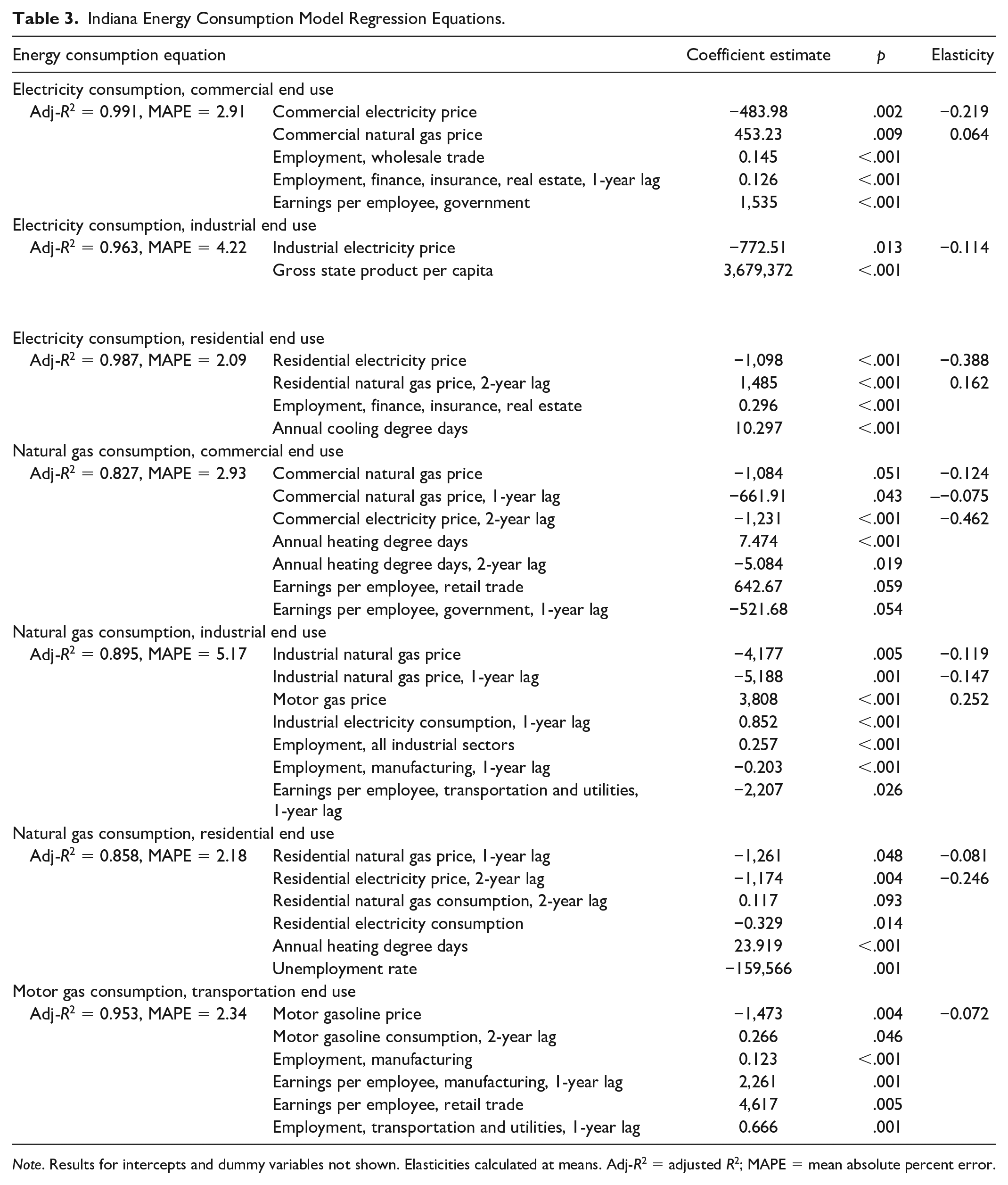
Note. Results for intercepts and dummy variables not shown. Elasticities calculated at means. Adj-R² = adjusted R²; MAPE = mean absolute percent error.

The performance of the predictive models is captured in two measurements: the adjusted R² and the MAPE. The adjusted R² is an indicator of how well the model specification reduces the variation in the dependent variable. Values in the range of 0.95 or higher are considered good, of 0.90 to 0.95 are fair, and of 0.80 to 0.90 are adequate. The MAPE is an indication of how well the model predicts actual observations over the sample period. Values in the range of 0% to 5% are excellent, 5% to 10% are very good, 10% to 15% are acceptable, and greater than 15% are suspect. Our results indicate generally excellent estimation results and sample period predictive performance. Predicted values over the sample period closely match peaks and troughs in the actual data, reflecting how our models capture turning points in the variables of interest (see Figure 1 for illustrations).

Figure 1.

Energy consumption for electricity, natural gas, and motor gas by end use in Indiana, 1979 to 2011, comparing actual data to values predicted by Indiana Scalable Economy and Energy Model (IN-SEEM).

Policy Relevance

The models for energy consumption are useful for policy analysis in several respects. First, the high performance and predictive ability ensure that simulations will result in scenario outputs that reflect historic relationships among the components of the model. Second, energy prices are crucial explanatory variables in these models. Econometric equations can, therefore, introduce a number of energy policies into the model by first, developing projections of energy prices under different scenarios, and second, introducing these projections exogenously through the price variables. These policy shocks—operationalized through price changes—then reverberate throughout the system of equations. Third, these equations reveal several relationships between energy consumption and the Indiana economy. These feedback loops between the energy sector and the economy are important for understanding the subtle, intricate, and unexpected ways by which energy policies—through their effect on prices—can affect the state economy, especially by identifying the relevance of particular sectors. More detailed data would be required to discern the mechanisms that make the different economic sectors sensitive to energy variables and nonintuitive relationships point to areas where further investigation would be fruitful. Fourth, the system of equations allows for direct modeling of energy policies on the economic variables themselves, in addition to the effects of policy on energy prices. Through the equations that predict individual sectoral economic variables, anticipated impacts to employment or wages can be introduced directly into the simulations. For example, if a mandate to install renewable generation capacity would result in the creation of a certain number of jobs in, say, the transportation and utilities sector, then employment in this sector can be increased by this exogenous number of jobs at some point in the simulation period, with subsequent effects reflected elsewhere in the system of equations, including in energy consumption. Together, these features capture the relevance of the energy sector for understanding potential policy scenarios. Such scenarios include carbon tax policies, gas tax policies, and other taxes affecting the energy sector, as well as any economic disruptions that increase or decrease electricity, natural gas, or gasoline prices. Thus, while IN-SEEM’s industrial structure does not differentiate between energy-based and nonenergy-based sectors or subsectors, it is still able to capture the effects of EBED activities through their anticipated effects on energy prices.

Application: A Policy Scenario Analysis

We demonstrate the relevance of IN-SEEM for policy analysis with an illustration of an exogenous policy shock to energy prices through Indiana’s short-lived DSM program. In 2009, the Indiana Utility Regulatory Commission (IURC) ordered the creation of Energizing Indiana, with the goal of reducing electricity consumption to 2% below 2008 levels by 2019 (IURC, 2009). Energizing Indiana would place a surcharge on customers’ bills to fund a variety of energy efficiency investments. According to a report early in the program (Kihm & Lord, 2014), the surcharge was projected to increase electricity prices by approximately 1%, 2%, and 3% on residential, commercial, and industrial customers, respectively. Shortly after implementation, critics claimed that industrial facilities enjoyed few energy savings, that any initial energy savings could not be sustained (McLaughlin, 2015), and that the overall effect of DSM was to make the state less economically competitive (M. R. Pence, personal communication, March 27, 2014). In 2014, the Indiana General Assembly canceled Energizing Indiana amid concerns that the surcharges were hurting the state economy.

The short life of Energizing Indiana makes it an appropriate illustration for IN-SEEM. The intended start of the program in 2011 coincides with the end of our sample period, and the 9-year time horizon fits within the acceptable range of a simulation period for top-down energy–economy models. We ran our model over the time period 2011 to 2019. The policy scenario consists of increased electricity prices as forecast by Kihm and Lord (2014). The abrupt end of Energizing Indiana contains the rationale for modeling this program solely in terms of prices. Despite evidence that DSM programs and energy efficiency measures are beneficial, both in general (Billingsley et al., 2014; Carley, 2012; Granade et al., 2009; National Academy of Sciences, 2010) and for Energizing Indiana specifically (Human, 2013; Kihm & Lord, 2014; TecMarket Works et al., 2013), legislators in Indiana concluded that the salient and overriding feature of the state’s DSM program was its effects on electricity prices.

Our policy scenario tests the logic by which the program was ended. Typically, reductions in energy consumption can occur through three paths: curtailment of energy services, substitution of labor for energy, or investment in alternative capital that is more energy efficient. IN-SEEM is able to model the former two, at least in an implicit way. Actual decisions about production and hiring may depend on a variety of factors, many of which are outside the scope of IN-SEEM. But by looking at historical relationships between energy prices and the rest of the economy, we capture these mechanisms in the absence of latent variables. As long as these mechanisms continue to operate in a constant way, we rely on IN-SEEM to predict how energy prices will lead to curtailment and labor substitutions.

Changes in capital are usually explicitly modeled in bottom-up models, but as a top-down model, IN-SEEM cannot currently do so. Therefore, our policy scenario represents a constrained implementation of DSM, whereby energy savings occur through price-induced curtailment, labor substitution, and endogenous technological substitution. This approximately captures a scenario wherein concerted efforts at capital investments are either economically or technologically infeasible—as suggested by the critics of Energizing Indiana. In certain sectors, however, it may be implausible that such capital investments are truly infeasible and our results may be helpful in distinguishing, as reflected in large projected changes in employment or wages, those sectors that deserve greater scrutiny: domain experts may be able to evaluate in which situations capital investments have a high potential for additional energy efficiency. As IN-SEEM currently lacks variables about interstate trade—in either the energy markets or other economic sectors—this policy scenario corresponds to a wholly intrastate shock to electricity prices.

Baseline Forecast

Our baseline forecast suggested a slight increase in employment of 1.9% between 2011 and 2019, though considerable variation is predicted across industry sectors (see Table 4). Employment growth over this period is projected for Finance, Insurance, and Real Estate; Services; Mining; Transportation and Utilities; and Government. Declines are anticipated in the Manufacturing, Construction, Retail, Wholesale Trade, and Farming sectors. The baseline forecast for average earnings per employee predicts a decrease (in real terms) of 5.5%, with slight increases in the Manufacturing and Government sectors and decreases in all other sectors. A real decrease in GSP per capita of 1.1% is predicted by the baseline forecast, along with a real increase in nonwage personal income per capita of 5.9%. The baseline forecast also suggested unemployment would increase from 9.4% to 9.5% between 2011 and 2019.

Table 4.

Results of Policy Analysis (Demand-Side Management Impacts Versus Baseline Scenario) for 2019.

	Baseline forecast	Policy forecast	Absolute difference	Percent difference
Gross state product, per capita	$42,688	$42,664	−$24	−0.06
Nonwage income, per capita	$17,205	$17,121	−$85	−0.49
Unemployment rate	9.43%	9.39%	0%	−0.42
Employment (jobs)
Construction	163,905	164,653	749	0.46
Farming	71,139	71,203	65	0.09
Manufacturing	347,254	350,478	3,224	0.93
Mining	13,318	13,307	−10	−0.08
Transportation and utilities	170,964	171,062	98	0.06
Subtotal: Industrial sectors	766,579	770,704	4,125	0.54
Finance, insurance, and real estate	316,214	315,904	−310	−0.10%
Government	482,076	481,299	−777	−0.16
Retail trade	355,851	355,035	−816	−0.23
Services	1,579,811	1,575,399	−4,413	−0.28
Wholesale trade	124,018	124,164	146	0.12
Subtotal: Commercial sectors	2,857,971	2,851,801	−6,170	−0.22
Total employment	3,624,550	3,622,504	−2,045	−0.06
Earnings per employee
Construction	$50,225	$50,332	$106	0.21
Farming	$36,171	$36,171	$0	0.00
Manufacturing	$26,422	$26,132	−$290	−1.10
Mining	$56,085	$56,038	−$47	−0.08
Transportation and utilities	$76,833	$76,805	−$27	−0.04
Finance, insurance, and real estate	$45,965	$46,375	$410	0.89
Government	$25,376	$25,438	$62	0.24
Retail trade	$37,855	$37,761	−$94	−0.25
Services	$52,864	$53,006	$142	0.27
Wholesale trade	$59,361	$59,118	−$243	−0.41
Average earnings per employee, total	$43,791	$43,769	−$23	−0.05
Electricity consumption (billion BTU)
Residential	122,096	120,978	−1,118	−0.92
Commercial	88,243	87,898	−345	−0.39
Industrial	160,170	159,937	−233	−0.15
Total electricity consumption	370,509	368,814	−1,695	−0.46
Natural gas consumption (billion BTU)
Residential	127,136	126,379	−757	−0.60
Commercial		75,061	−585	−0.77
Industrial	339,821	339,699	−122	−0.04
Total natural gas consumption	542,604	541,139	−1,465	−0.27
Motor gasoline consumption (billion BTU)	351,220.89	351,901.21	680	0.19

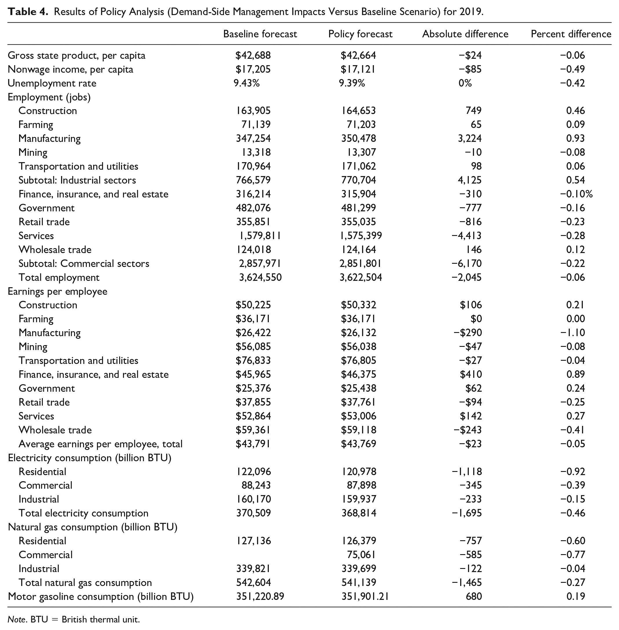
Note. BTU = British thermal unit.

The baseline forecast predicted significant variation in the rate of change of energy consumption by type and end-use sector. Residential and commercial electricity consumption were projected to increase by 7.4% and 6.8%, respectively, while industrial electricity consumption was forecast to decline by 1.4%. Industrial natural gas consumption, meanwhile, was projected to rise by 7.4%, with 5.8% and 1.5% declines in residential and commercial natural gas consumption, respectively. The baseline model also predicted a 3.3% decrease in motor gasoline consumption.

Policy Impact

The results from the policy scenario reveal several important differences from the baseline scenario. Primarily, we see the projected changes in electricity consumption depicted in Figure 2. Without targeted investments in technological substitution, most electricity consumption is projected to continue to increase above 2008 levels. The exception is the industrial end use, which decreases due to secular trends in other exogenous variable projections. The price changes under the policy scenario, however, do reduce consumption below the reference scenario. The size of this difference varies among end uses: For residential customers, a 1% increase in electricity prices will induce an average 0.92% reduction over the program period; for commercial customers, a 2% price increase induces 0.45% reduction; and for industrial customers, a 3% increase induces a 0.10% reduction. In total, the price changes are projected to induce an average 0.44% reduction in electricity consumption relative to the baseline forecast. Despite these savings, prices alone do not change the slope of the electricity consumption trends. Dividing the total revenue generated by the surcharge over the total electricity savings over the simulation period yields a private cost of 29¢ per kilowatt-hour saved. Thus, the analysis suggests the DSM program is a costly endeavor, at least in the near term, as the substantial amount of additional revenue collected from the increased electricity prices is spread out over a relatively small reduction in consumption.

Figure 2.

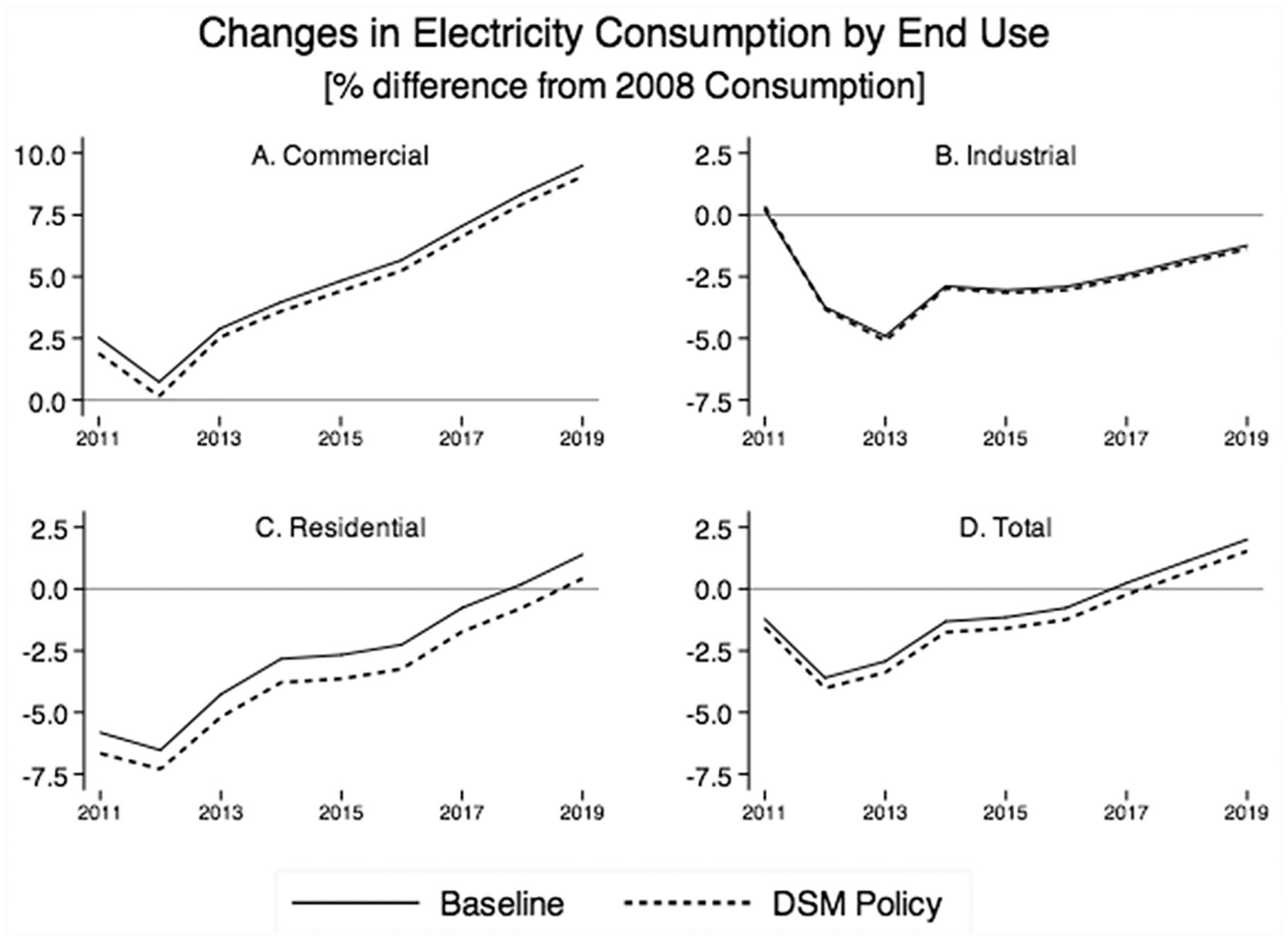
Projections of changes in electricity consumption for different end uses in Indiana, 2011 to 2019, under the baseline and demand-side management (DSM) policy scenarios, using 2008 as the base year. The stated goal of the DSM policy is a reduction of 2% below 2008 levels by 2019.

Beyond energy savings, we also explore the economic impacts from the price changes. Table 4 shows the differences for each endogenous variable between the baseline and policy forecasts at the end of the program in 2019, in both absolute and relative terms. Among the macroeconomic indicators, we find that the policy scenario includes a negative but modest impact on the state economy, with small drops in per capita GSP and nonwage income; the unemployment rate, on the other hand, drops slightly. A richer picture emerges when considering the sectoral impacts. Among industrial sectors, the price increase appears to increase employment and earnings per employee—the exceptions being employment in Mining and earnings per employee in Manufacturing. The commercial sectors see reductions in both employment and earnings per employee—the only exception being employment in the Wholesale Trade sector. The data in the current version of IN-SEEM provided cannot explain the mechanisms that produce the different effects among the economic sectors, yet they are theoretically plausible. Employment gains in Manufacturing and Construction suggest labor-energy substitutions; for example, the replacement of manpower for power tools or increased effort at maintenance of machinery to improve its energy efficiency. Job losses in Retail Trade and Services, on the other hand, suggest curtailment, as increased electricity costs may be lowering economic activity. Richer subnational data, or qualitative analysis, could provide further context for model results. With respect to other energy carriers, the policy scenario shows decreased consumption across all three end uses of natural gas, most especially commercial. Motor gasoline consumption increases under the policy scenario.

Discussion and Conclusion

In this analysis, we sought to develop a model that allows researchers to consider the effects of changes in energy prices stemming from energy and climate policies, as well as EBED activities, on state economies. This degree of microeconomic realism and geographic specificity, we argue, is particularly important in an era in which state and local governments are helping to lead U.S. energy policy. As a proof of concept, we built the IN-SEEM for the state of Indiana and then illustrated its performance with a policy application related to the state’s DSM program.

Our policy analysis illustration offers several lessons for policy makers and practitioners. First, prices alone are insufficient to generate the electricity savings goal of Energizing Indiana. Through curtailment and endogenous technological substitution, the price increases cut electricity consumption by less than half a percent over the baseline and fail to set the state on a trajectory for an ultimate goal of 2% below 2008 levels. Over the short term, it is not apparent that any implicit investments in energy-saving technologies are yielding dividends, though there may be substantial energy savings in the longer term.

Second, while the price increases do have negative effects on the economy of the state, these costs are relatively small, most notably an approximate loss in GSP per capita of $24 by the end of the program in 2019. The values for employment and the unemployment rate suggest that the industrial sectors, in particular, respond to the price increases by substituting labor for electricity. Commercial customers may have fewer such opportunities for mitigating increases in electricity prices, leading to curtailment instead. Overall, the negative effects of increased electricity prices on the state economy are modest and likely to be less influential than other factors unrelated to this energy policy. The potential benefits of DSM, on the other hand, may be more substantial.

Third, because IN-SEEM is a top-down model without an explicit means of capturing technological change, the policy analysis results may fail to fully capture all the effects of a DSM program. If, for instance, price increases in the real world induce a switch from traditional fossil fuel-based technologies to renewable energy technologies, such a shift would not show up in the simulation results. Over the near term—as is the case in this policy analysis—this is not a major concern. However, over longer periods of time—when technological change is more likely to occur – the current structure and capabilities of IN-SEEM may fall short. This is particularly important if our approach is applied to states with a more varied energy technology mix. In Indiana, electricity typically means coal; but in the Pacific Northwest, hydro makes up a significant share of the electricity generation pie. Other states generate significant shares of electricity from wind and solar. Because our modeling approach makes forecasts based on historic relationships among the available variables, such an approach may falter in states with larger shares of alternative energy capacity unless historical data permit a researcher to include equations for additional energy types.

Given the policy analysis results of the application of IN-SEEM, this research study mainly serves as a proof of concept for the regional econometric modeling approach to policy analysis in this field. The increase in electricity prices analyzed in this article is just one of many scenarios that could be examined. The impacts of any national- or state-level policy that affects energy prices or consumption can be analyzed through this approach. Examples include carbon taxes, other taxes on consumption or production, subsidies, expansion or contraction of the supply of various fuels, and renewable portfolio standards. Subnational econometric models also lend themselves to extensions such as integration with technological models—including MARKALand geospatial data on land use, infrastructure constraints, and environmental impacts. These extensions illustrate the usefulness of this modeling framework for geographic specificity and macroeconomic completeness. Such levels of sophistication are necessary to provide policy makers and stakeholders with useful research into the possible impacts of the climate and energy policies that have proliferated at the state and local levels.

Supplemental Material

EDQ-18-0071-R2-Appendix – Supplemental material for A Scalable Energy–Economy Model for State-Level Policy Analysis Applied to a Demand-Side Management Program

Supplemental material, EDQ-18-0071-R2-Appendix for A Scalable Energy–Economy Model for State-Level Policy Analysis Applied to a Demand-Side Management Program by Zachary A. Wendling, David C. Warren, Barry M. Rubin, Sanya Carley and Kenneth R. Richards in Economic Development Quarterly

Footnotes

Acknowledgements

The authors would like to thank J. C. Randolph, Farah Abi-Akar, Joanna Allerhand, David C. Gehl, Ed Gerrish, and John Rupp for assistance.

Declaration of Conflicting Interests

The author(s) declared no potential conflicts of interest with respect to the research, authorship, and/or publication of this article.

Funding

The author(s) disclosed receipt of the following financial support for the research, authorship, and/or publication of this article: This research has been generously supported by Indiana University through the President’s Fund, the School of Public and Environmental Affairs, the Center for Research in Energy and the Environment, and the Office of the Vice Provost for Research.

ORCID iD

David C. Warren

Supplemental Material

Supplemental material for this article is available online.

Notes

Author Biographies

Zachary A. Wendling is a postdoctoral associate at the Yale Center for Environmental Law & Policy and the principal investigator of the Environmental Performance Index. He studies energy and environmental policy, especially the importance of data and metrics.

David C. Warren is a founding partner of Cardinal Analytics and Planning Associates in Bloomington, Indiana. He recently earned his PhD from the O’Neill School of Public and Environmental Affairs at Indiana University, where he also teaches a class on local government.

Barry M. Rubin is professor emeritus at the O’Neill School of Public and Environmental Affairs and a founding partner of Cardinal Analytics and Planning Associates. His research includes urban and regional economic development, state-level energy policy analysis, strategic planning, and management.

Sanya Carley is a professor at the O’Neill School of Public and Environmental Affairs at Indiana University. Her research focuses on electricity and transportation policies.

Kenneth R. Richards is a professor of environmental economics and policy at the O’Neill School of Public and Environmental Affairs and an affiliated professor of law at the Indiana University Maurer School of Law.

References

Billingsley

M. A.

Hoffman

I. M.

Start

Schiller

S. R.

Goldman

C. A.

LaCommare

(2014). The program administrator cost of saved energy for utility customer-funded energy efficiency programs (No. LBNL-6595E). Lawrence Berkeley National Laboratory. https://doi.org/10.2172/1129528

Blanford

G. J.

Merrick

J. H.

Young

(2014). A clean energy standard analysis with the US-REGEN model. The Energy Journal, 35(S01), 137-164. https://doi.org/10.5547/01956574.35.SI1.8

Brandsma

Kancs

(2015). RHOMOLO: A dynamic general equilibrium modelling approach to the evaluation of the European Union’s R&D policies. Regional Studies, 49(8), 1340-1359. https://doi.org/10.1080/00343404.2015.1034665

Brandsma

Kancs

d’A.

Monfort

Rillaers

(2015). RHOMOLO: A dynamic spatial general equilibrium model for assessing the impact of cohesion policy. Papers in Regional Science, 94(Suppl. 1), S197-S221. https://doi.org/10.1111/pirs.12162

Bushnell

Peterman

Wolfram

(2007). Local solutions to global problems: Policy choice and regulatory jurisdiction [National Bureau of Economic Research Working Paper Series, No. 13472]. http://www.nber.org/papers/w13472

California Energy Commission. (2017a). Electricity consumption by county. http://ecdms.energy.ca.gov/elecbycounty.aspx

California Energy Commission. (2017b). Gas consumption by county. http://ecdms.energy.ca.gov/gasbycounty.aspx

Carley

(2011). The era of state energy policy innovation: A review of policy instruments. Review of Policy Research, 28(3), 265-294. https://doi.org/10.1111/j.1541-1338.2011.00495.x

Carley

(2012). Energy demand-side management: New perspectives for a new era. Journal of Policy Analysis and Management, 31(1), 6-32. https://doi.org/10.1002/pam.20618

10.

Carley

Lawrence

Brown

Nourafshan

Benami

(2011). Energy-based economic development. Renewable and Sustainable Energy Reviews, 15(1), 282-295. https://doi.org/10.1016/j.rser.2010.08.006

11.

Chen

Wiser

Mills

Bolinger

(2009). Weighing the costs and benefits of state renewables portfolio standards in the United States: A comparative analysis of state-level policy impact projections. Renewable and Sustainable Energy Reviews, 13(3), 552-566. https://doi.org/10.1016/j.rser.2008.01.005

12.

Collins

A. R.

Hansen

Hendryx

(2012). Wind versus coal: Comparing the local economic impacts of energy resource development in Appalachia. Energy Policy, 50, 551-561. https://doi.org/10.1016/j.enpol.2012.08.001

13.

Considine

Manderson

(2013). Balancing fiscal, energy, and environmental concerns: Analyzing the policy options for california’s energy and economic future. Energies, 6(3), 1266-1297.

14.

Coon

R. C.

Hodur

N. M.

Bangsund

D. A.

(2012). Renewable energy industries contribution to the North Dakota Economy (Agribusiness and Applied Economics Report No. 702; Agribusiness and Applied Economics Report). http://ageconsearch.umn.edu/bitstream/140122/2/AAE702.pdf

15.

Electric Power Research Institute. (2014). US-REGEN model documentation (Technical Report 3002004693). EPRI.

16.

Gabriel

S. A.

Kydes

A. S.

Whitman

(2001). The national energy modeling system: A large-scale energy-economic equilibrium model. Operations Research, 49(1), 14-25. https://doi.org/10.1287/opre.49.1.14.11195

17.

Goldsmith

(2000). The ISER Alaska input-output model. (ISER Working Paper 98.1, revised April). https://kidscount.alaska.edu/ISER/Publications/workingpapers/WP_98.1_ISER_AK_Input-Output%20Model.pdf

18.

Granade

H. C.

Creyts

Derkach

Farese

Nyquist

Ostrowski

(2009). Unlocking energy efficiency in the US economy. McKinsey.

19.

Grubb

Köhler

Anderson

(2002). Induced technical change in energy and environmental modeling: Analytic approaches and policy implications. Annual Review of Energy and the Environment, 27(1), 271-308. https://doi.org/10.1146/annurev.energy.27.122001.083408

20.

Hourcade

J.-C.

Jaccard

Bataille

Ghersi

(2006). Hybrid modeling: New answers to old challenges. Introduction to the special issue of “ The Energy Journal.” Energy Journal, 1-11. https://doi.org/10.5547/ISSN0195-6574-EJ-VolSI2006-NoSI2-1

21.

Human

(2013, August 19). Utilities fall short on efficiency spending. Indianapolis Business Journal, pp. 1, 22.

22.

Indiana Utility Regulatory Commission. (2009). Cause Number 42693.

23.

Jaccard

(2005). Hybrid energy-economy models and endogenous technological change. In Energy and environment (pp. 81-109). Springer. https://doi.org/10.1007/0-387-25352-1_4

24.

Jaccard

Nyboer

Bataille

Sadownik

(2003). Modeling the cost of climate policy: distinguishing between alternative cost definitions and long-run cost dynamics. Energy Journal, 24(1), 49-73.

25.

Jones

Kane

S. P.

McKissick

J. C.

(2010). An estimation of the potential impact on Georgia’s economy of higher energy costs predicted under the Cap and Trade Provisions of HR 2454. Journal of Agribusiness, 28(2), 183-202.

26.

Khadka Mishra

. (2009). Estimation of externality costs of electricity generation from coal: An OH-MARKAL extension [Electronic Thesis or Dissertation]. http://rave.ohiolink.edu/etdc/view?acc_num=osu12597033377

27.

Kihm

Lord

(2014). Indiana’s core and core plus energy efficiency programs: Benefits, costs, and savings. Energy Center of Wisconsin.

28.

Kim

S. H.

Edmonds

Lurz

Smith

S. J.

Wise

(2006). The objECTS Framework for integrated assessment: Hybrid modeling of transportation. The Energy Journal, SI2006(01). https://doi.org/10.5547/ISSN0195-6574-EJ-VolSI2006-NoSI2-4

29.

Preckel

P. V.

Gotham

Liu

A. L.

(2016). An assessment of alternative carbon mitigation policies for achieving the emissions reduction of the clean power plan: Case study for the state of Indiana. Energy Policy, 96, 661-672. https://doi.org/10.1016/j.enpol.2016.06.045

30.

McCollum

Yang

Yeh

Ogden

(2012). Deep greenhouse gas reduction scenarios for California – Strategic implications from the CA-TIMES energy-economic systems model. Energy Strategy Reviews, 1(1), 19-32. https://doi.org/10.1016/j.esr.2011.12.003

31.

McLaughlin

(2015, January 8). Pence proposes utilities set own energy-efficiency goals. Indianapolis Business Journal. http://www.ibj.com/articles/51220-pence-proposes-utilities-set-own-energy-efficiency-goals

32.

Mehmood

S. R.

Pelkki

M. H.

(2009). Economic impacts of future biorefineries in the state of Arkansas: An input-output analysis. Journal of the Arkansas Academy of Science, 63, 195-197.

33.

Miller

Wei

Rose

(2010). The macroeconomic impact of the Michigan climate action council climate action plan on the state’s economy. The Center for Climate Strategies. http://www.michigan.gov/documents/dnre/dnre-Climate-action-ECON-Impacts_340497_7.pdf

34.

Montgomery

W. D.

Baron

Bernstein

Harrison

Mankowski

McPhail

Tuladhar

S. D.

Xiong

Yuan

(2014). Socio-economic impact analysis of Alaska LNG Project. NERA Economic Consulting.

35.

Murray

B. C.

Pizer

W. A.

Ross

M. T.

(2015). Regulating existing power plants under the U.S. Clean Air Act: Present and future consequences of key design choices. Energy Policy, 83, 87-98. https://doi.org/10.1016/j.enpol.2015.03.028

36.

National Academy of Sciences. (2010). Real prospects for energy efficiency in the United States. National Academies Press.

37.

Pence

M. R.

(2014, March 27). Letter to Legislative Leaders on SEA340.

38.

Pollitt

Alexandri

Chewpreecha

Klaassen

(2015). Macroeconomic analysis of the employment impacts of future EU climate policies. Climate Policy, 15(5), 604-625. https://doi.org/10.1080/14693062.2014.953907

39.

Pollitt

Chewpreecha

Summerton

(2007). E3ME: An energy–environment–economy model for Europe. http://www.petre.org.uk/pdf/E3ME_Technical_Description_v4.2.pdf

40.

Rabe

B. G.

(2008). States on steroids: the intergovernmental odyssey of American climate policy. Review of Policy Research, 25(2), 105-128. https://doi.org/10.1111/j.1541-1338.2007.00314.x

41.

Regional Economic Models, Inc. (2007). REMI Policy Insight 9.5 Model Documentation.

42.

Rivers

Jaccard

(2005). Combining top-down and bottom-up approaches to energy-economy modeling using discrete choice methods. Energy Journal, 26(1), 83-106. https://doi.org/10.5547/ISSN0195-6574-EJ-Vol26-No1-4

43.

Roland-Holst

(2008). Energy efficiency, innovation, and job creation in California. Center for Energy, Resources, and Economic Sustainability.

44.

Roland-Holst

(2010). Real incomes, employment, and California Climate Policy (Research Paper No.1007241). Center for Energy, Resources, and Economic Sustainability.

45.

Roland-Holst

(2011). More jobs per gallon: How vehicle efficiency fuels growth in California (Research Paper No. 1103011). Center for Energy, Resources, and Economic Sustainability.

46.

Rose

Wei

(2009). The economic impact of the Florida energy and climate change action plan on the State’s Economy. UCLA Center for Climate Strategies. http://www.climatestrategies.us/library/library/view/756

47.

Rose

Wei

Dormady

(2011). Regional macroeconomic assessment of the Pennsylvania climate action plan: Macroeconomics of climate action planning. Regional Science Policy & Practice, 3(4), 357-379. https://doi.org/10.1111/j.1757-7802.2011.01048.x

48.

Rose

Wei

Prager

(2012). Impacts of climate policy on the California Economy. http://next10.org/sites/next10.org/files/Rose_Final.pdf

49.

Ross

M. T.

(2008). Documentation of the applied dynamic analysis of the Global Economy (ADAGE) Model (Working Paper 08_01). Research Triangle Institute.

50.

Ross

M. T.

(2014a). Structure of the dynamic integrated economy/energy/emissions model: Computable general equilbrium component, DIEM-CGE (Working Paper NI WP 14-12). Nicholas Institute for Environmental Policy Solutions.

51.

Ross

M. T.

(2014b). Structure of the dynamic integrated economy/energy/emissions model: Electricity component, DIEM-electricity (Working Paper NI WP 14-11). Nicholas Institute for Environmental Policy Solutions.

52.

Ross

M. T.

Hoppock

Murray

B. C.

(2015). Assessing impacts of the clean power plan on Southeast states (Working Paper NI WP 15-03). Nicholas Institute for Environmental Policy Solutions. http://nicholasinstitute.duke.edu/publications

53.

Ross

M. T.

Hoppock

Murray

B. C.

(2016). Ongoing evolu-tion of the electricity industry: Effects of market conditions and the clean power plan on states (Working Paper NI WP 16-07). Nicholas Institute for Environmental Policy Solutions. http://nicholasinstitute.duke.edu/ publications

54.

Ross

M. T.

Murray

B. C.

(2016). What is the fuel of the future? Prospects under the clean power plan. Energy Economics, 60, 451-459. https://doi.org/10.1016/j.eneco.2016.09.021

55.

Ross

M. T.

Murray

B. C.

Beach

R. H.

Depro

B. M.

(2008). State-level economic impacts of a National Climate Change policy. Pew Center on Global Climate Change.

56.

Ross

M. T.

Murray

B. C.

Hoppock

(2015). The clean power plan: Implications of three compliance decisions for U.S. states (Working Paper NI WP 15-02). Nicholas Institute for Environmental Policy Solutions. http://nicholasinstitute.duke.edu/publications

57.

Rubin

B. M.

Hilton

M. D.

(1996). Identifying the local economic development impacts of global climate change. Economic Development Quarterly, 10(3), 262-279. https://doi.org/10.1177/089124249601000306

58.

Rubin

B. M.

Gailmard

Marsh

Septoff

(1997). Assessing the state-level consequences of global warming: Socioeconomic and energy demand impacts. World Resource Review, 9(3), 379-387.

59.

Shakya

B. S.

(2007). Biomass resources for energy in Ohio: The OH-MARKAL modeling framework. [Electronic Thesis or Dissertation]. http://rave.ohiolink.edu/etdc/view?acc_num=osu1180118764

60.

Short

Sullivan

Mai

Mowers

Uriarte

Blair

Heimiller

Martinez

(2011). Regional energy deployment system (ReEDS) (Technical Report NREL/TP-6A20-46534). National Renewable Energy Laboratory.

61.

Slattery

M. C.

Lantz

Johnson

B. L.

(2011). State and local economic impacts from wind energy projects: Texas case study. Energy Policy, 39(12), 7930-7940. https://doi.org/10.1016/j.enpol.2011.09.047

62.

Solomon

B. D.

Rubin

B. M.

(1997). Environmental linkages in regional econometric models: an analysis of coal development in Western Kentucky. Land Economics, 62(1), 43-57. https://doi.org/10.2307/3146139

63.

Tuladhar

S. D.

Montgomery

W. D.

Kaufman

(2015). Environmental policy for fiscal reform: Can a carbon tax play a role? National Tax Journal, 68(1), 179-194. https://doi.org/10.17310/ntj.2015.1.08

64.

Wei

Patadia

Kammen

D. M.

(2010). Putting renewables and energy efficiency to work: How many jobs can the clean energy industry generate in the US? Energy Policy, 38(2), 919-931. https://doi.org/10.1016/j.enpol.2009.10.044

65.

Wiser

Porter

Clemmer

(2000). Emerging markets for renewable energy: The role of state policies during restructuring. Electricity Journal, 13(1), 13-24. https://doi.org/10.1016/S1040-6190(99)00101-3

Supplementary Material

Please find the following supplemental material available below.

For Open Access articles published under a Creative Commons License, all supplemental material carries the same license as the article it is associated with.

For non-Open Access articles published, all supplemental material carries a non-exclusive license, and permission requests for re-use of supplemental material or any part of supplemental material shall be sent directly to the copyright owner as specified in the copyright notice associated with the article.

0.00 MB

0.30 MB

A Scalable Energy–Economy Model for State-Level Policy Analysis Applied to a Demand-Side Management Program

Abstract

Keywords

Energy–Economy Modeling

Top-Down Versus Bottom-Up

The Indiana Scalable Energy–Economy Model

Methodological Approach

Data

Model and Modeling Approach 3

Applying the Econometric Systems of Equations to Other States

IN-SEEM Performance

Policy Relevance

Application: A Policy Scenario Analysis

Baseline Forecast

Policy Impact

Discussion and Conclusion

Supplemental Material

EDQ-18-0071-R2-Appendix – Supplemental material for A Scalable Energy–Economy Model for State-Level Policy Analysis Applied to a Demand-Side Management Program

Footnotes

Acknowledgements

Declaration of Conflicting Interests

Funding

ORCID iD

Supplemental Material

Notes

Author Biographies

References

Supplementary Material

Model and Modeling Approach³