
Abstract
This article outlines a practical standard of university economic impact analyses for small colleges. The needs of small colleges greatly differ from those of large universities, as they are typically dependent on in-house resources to conduct economic impact analyses. These financial limitations create a need for suitable, publicly available data that can substitute for primary, costly data collection, as well as guidelines on best practices for researchers or practitioners who may not be experts in input–output methodology. The article reviews the foundations of economic impact analysis and then discusses fundamental modeling decisions. The suggested practices are illustrated using two small colleges in Ohio as case studies.
There are a myriad of studies that focus on the economic impact of universities and colleges and how they contribute to the economic vitality of their surrounding regions and states. While this focus is wide, encompassing everything from examining urban colleges (Steinacker, 2005) to looking at the draw of sports and athletic events (Baade et al., 2008, 2011), less work has addressed the impact of small colleges. In addition, since the model estimating the impact of colleges and universities was published almost 50 years ago (Caffrey & Isaacs, 1971), the process of modeling economic impacts has become more complex and commercialized, while its use has become more common.
One of the main criticisms of economic impact analysis as an analytical tool used to estimate economic benefits for an industry, organization, or policy is that the results are highly dependent on both the assumptions made by researchers and the methodologies used. For example, models can overestimate the impacts on the local economy when they include an erroneous definition of “new” dollars spent by students or visitors into the local region (Bluestone, 1993). Furthermore, there is no consensus on the validity of including universities’ and colleges’ monetary estimates of the human capital buildup when conducting such analyses (Beck et al., 1995; Bluestone, 1993). The impacts sustained by an increased supply of human capital and greater innovation are vital contributions (Abel & Deitz, 2011; Valero & Van Reenen, 2019). However, quantifying the value of human capital buildup for a single university remains a challenging task. Economic impact analyses often either mention these ancillary impacts without measuring them (Bailey et al., 2007) or use the income added in the region by former students as a proxy for the increase in a regional economy’s stock of human capital (Economic Modeling Specialists International [EMSI], 2017).
This article provides a practical standard of university economic impact methods, while also focusing on the needs of small colleges. These colleges must often rely on in-house resources (e.g., professors or economic development professionals on the payroll). This article can be used as a guide by small colleges to identify accessible data and best practices, thus producing economic impact analyses that fit within their budget. Economic impact studies are valuable tools for colleges and universities as they seek funding, since such studies can demonstrate the importance of the university or college to the overall economy. Moreover, economic impact analyses can increase external awareness of the organization, strengthen relationships with various stakeholders, and assist in marketing and public relations. Studies have found that institutions of higher education use these analyses to self-promote and appeal to outside funders (French, 2019). For example, the United Fund (2021), which provides financial support to African American students, commissioned a study of the economic impact of historically Black colleges and universities to demonstrate this value to both funders and member institutions. These studies are also used to demonstrate impact to local governments, as public and private colleges do not pay property taxes in many jurisdictions (Siegfried et al., 2007).
Throughout this article, to quantify the economic value of a college to its region, the economic impact analysis will model a university’s impact through multiple channels: (a) operating expenses, (b) student spending, (c) visitor spending, and (d) construction expenses. The decision to model these four channels relies on established best practices for measuring the value of universities and colleges to regional economies (Ambargis et al., 2014; Swenson, 2015). University expenses can be used as a measure of university operations. For smaller colleges with limited budgets, to avoid substantial survey costs, student spending can be based on the actual spending pattern of full-time students nationally, as measured by the annual Consumer Expenditure Survey. Student spending that occurs as part of university operations (e.g., payments for on campus residency) should be excluded to ensure no double counting. Similarly, visitor spending can be estimated using the standard room and per diem reimbursement rates for a region from the U.S. General Services Administration. Construction expenses can be based either on the college’s spending on a new building or buildings in a given year or on average construction expenses over a range of years. Furthermore, it should be noted that no attempt was made to quantify any potential benefit from an increase in human capital or other benefits accruing because of the presence of a university in the region. Such benefits are difficult to value and remain based on assumptions that, but for these particular universities, said benefits would not exist.
The researchers illustrate their suggested practices using two institutions of higher education in Ohio as examples: Marietta College and Muskingum University. The numbers from these two institutions were inputted into IMPLAN: Economic Impact Analysis for Planning (Clouse, 2020b), which can be utilized to estimate the overall economic impacts that are due to a college’s activities. IMPLAN employs an economic modeling technique called input–output (I-O) analysis, which is a type of applied economic analysis that tracks the interdependence among various producing and consuming industries of an economy. It measures the relationship between a given set of demands for final goods and services as well as the inputs required to satisfy those demands (Clouse, 2020b). For example, when the college purchases supplies from a local vendor, that local vendor provides wages to its employees and makes purchases from other vendors. These other vendors in turn provide wages to their employees, make purchases from other vendors, and so on. Additionally, when employees of the university spend their paychecks at local businesses, these local businesses provide wages to their employees, make purchases from other vendors, and the cycle continues. As a result, the initial dollars spent by the university will be circulated throughout the local economy multiple times, and this amount can be estimated using economic multipliers.
Subsequent sections of this article proceed as follows. Section 2 describes the foundations of economic impact analysis by reviewing I-O methodology, explains the indicators produced by the analysis, and provides a synthesis of the differences between currently available economic impact analysis software programs. Section 3 then discusses economic impact analysis design, and key modeling decisions, offering Marietta College and Muskingum University as examples.
The Foundation of Economic Impact Analysis
Scholars have already noted the prevalence of too much variation in the methodology used when examining the economic impact of universities (Beck et al., 1995; Drucker & Goldstein, 2007). For example, a 2015 analysis examining the economic impact of Wisconsin Lutheran College used IMPLAN and modeled university-level information, including capital expenditures, operational expenditures, and jobs (Tripp Umbach, 2015). Conversely, a 2019 analysis examining the economic impact of Pace University (2019) used Regional Input–Output Modeling System (RIMS II) and modeled student and visitor spending in addition to university spending. The difference in methodologies and components potentially reflects the difference in researchers’ preferences, as one analysis was created by a consultant and the other was an in-house production. This variation not only generates concerns around proper methodologies, but also makes it impossible to compare results across analyses. The following subsections go on to explore the foundation of economic impact analyses.
Input–Output Analysis
Traditional economic impact analysis utilizes I-O models that date back to the 1940s and the work of Wassily Leontief (Day, 2015). These models focused on the financial exchange of products and services between industries, households, and governments (Watson et al., 2007). They provided a detailed description of the economy, thus allowing for the estimation of economic impacts due to input changes that mirrored changes in a region, such as a new plant opening (Day, 2015; Leontief, 1986). I-O models now reflect the most recently available year’s data and are mostly subject to assumptions inherent in the models’ structure. These include stationarity, constant returns to scale, unconstrained supply, fixed input structures, static industry and commodity technology, and constant byproducts of industries (Clouse, 2020b).
There are four main sources of commercial I-O models typically used in economic impact studies: (a) IMPLAN, (b) RIMS II, (c) Regional Economic Models Incorporated (REMI), and (d) EMSI. All utilize I-O modeling. However, the values of the multipliers used differ, with IMPLAN having higher estimated multipliers than RIMS II, REMI, or EMSI (Bess & Ambargis, 2011; Kim & Miller, 2016; Rickman & Schwer, 1995). Another variance across these sources is the number of sectors included in the models (Kim & Miller, 2016).
Furthermore, these four sources of I-O models differ in the geographic level of analysis they allow. IMPLAN, born out of the U.S. Forest Service (Clouse, 2020a), can analyze economies at the zip code, congressional district, county, metropolitan statistical area (MSA), state, and national levels (Day, 2015). The RIMS II, created and maintained by the Bureau of Economic Analysis (BEA), can analyze economies at the city, county, or MSA level (Bess & Ambargis, 2011). The REMI model, owned by Regional Economic Models Incorporated, is a more robust model that combines I-O modeling and general equilibrium models (REMI, 2016). It can analyze economies at the county, state, and national levels (Bonn & Harrington, 2008). Last, the EMSI, also allows for modeling at the zip code, city, county, and state levels (Kim & Miller, 2016).
These commercial I-O models each have their own set of different advantages and drawbacks. The models utilize different data sources and different modeling techniques to identify multipliers (AKRF, 2013; Galloway, 2007; Lynch, 2000; Rickman & Schwer, 1995). RIMS II, the least expensive program, uses location quotients to transform national-level coefficients into a regional scale for analysis (Galloway, 2007). This model assumes that the region will satisfy local demand before accounting for foreign demand or exports, hence tending to generate an overestimated regional multiplier, since businesses typically export much of their product (Galloway, 2007). Unlike RIMS II, the IMPLAN model uses interstate trade flow matrices in addition to a region’s demand and supply–demand ratios to determine multipliers. Although this is considered a more advanced approach, it limits the I-O model’s ability to properly account for industries that are added to the region by restricting the regional purchase coefficients (Galloway, 2007).
Recognized as even more precise—and consequently more expensive—is the REMI model that employs the Stevens technique, a practice lauded as the superior method since it accounts for local business patterns when measuring regional purchase coefficients, or RPCs (Galloway, 2007). Last, the EMSI model uses a similarly elevated technique as REMI but allows for a more dynamic model that accounts for new industries in local regions as well as industry growth (Galloway, 2007).
Among other distinctions, IMPLAN and REMI are cited as being more user friendly, whereas RIMS II can be challenging to work with (Lynch, 2000). REMI is a dynamic model that accounts for economic patterns across time and the complexity of the real world (AKRF, 2013), while IMPLAN is best equipped to handle modeling for multiple regions as well as smaller areas of study. In addition, IMPLAN includes a descriptive breakdown of impacts by industry and allows for industry customization (AKRF, 2013; Day, 2015). RIMS II is simple; hence, it lacks some of the advantages inherent when other I-O models are employed (AKRF, 2013).
Key to economic impact analyses is the concept of multipliers derived from I-O tables. Multipliers are ratios of the total and partial changes in the economy that account for interindustry relationships (Bess & Ambargis, 2011); they rely on statistical estimations based on the size of an area in addition to the diversity of goods and services it produces (Caffrey & Isaacs, 1971). This economic model expresses the number of additional jobs or amount of additional income created by each new job or extra dollar earned. Consequently, these multipliers, which estimate the “ripple effect” of money flowing through the local economy, will be larger when there is less money leakage out of the region of study (Caffrey & Isaacs, 1971).
Economic Indicators
These four I-O models also differ in the sets of economic indicators they produce. For example, economic impact analysis using IMPLAN consists of five indicators: (a) employment, (b) labor income, (c) value added, (d) output, and (e) taxes (Day, 2015). Employment considers the number of full-time and part-time persons employed within the study area, including proprietors, who are supported by the university’s or college’s spending. Labor income represents the total value of all forms of employment income. Value added, a measure of the contribution to gross domestic product (GDP), represents the difference between output and the cost of intermediate inputs. “Output” refers to the value of production by industry in a calendar year generated within the study area because of the presence of the university or college (Clouse, 2020a). Last, taxes measure federal, state, and local tax revenues resulting from the university or college. These products of IMPLAN cannot be added together and should remain separate when reporting results (Day, 2015).
The RIMS II model indicators are similar to the IMPLAN indicators, but they do not include taxes. These products are (a) employment, (b) earnings, (c) value added, and (d) output (Bess & Ambargis, 2011). Employment is the number of jobs for both full-time and part-time employees, again including proprietors (Bess & Ambargis, 2011). It refers to a person’s years of employment regardless of the term over which the spending input is aggregated (Lynch, 2000). When earnings are calculated using RIMS II, benefits are included. Other variables included in earnings are wages, salaries, and proprietors’ incomes, all akin to the IMPLAN model (Bess & Ambargis, 2011). Value added, calculated by subtracting the intermediate inputs from the gross output, is thus equivalent to the total sum of taxes and imports (not including subsidies), any output surplus, and the compensation of employees (Bess & Ambargis, 2011). Gross output is the sum of intermediate inputs and value added (Bess & Ambargis, 2011).
The EMSI model builds on IMPLAN and RIMS II in that, in addition to estimating measures of economic growth, jobs, and earnings by industry, it provides a description of the supply chain (Kim & Miller, 2016). As with the other models, EMSI earnings include proprietor earnings (Crapuchettes et al., 2019). Finally, I-O models provide different levels of multipliers, also known as types. Type I looks at industry-to-industry transactions in addition to direct and indirect impacts, but it does not include induced effects. Type II and Type SAM build on Type I by introducing these induced effects of households. EMSI goes one step further, forming its own type that factors in the effects addressed by Type II models as well as additional investment that impacts the economy. As such, EMSI accounts for business purchases, such as new equipment or buildings, and spending by the government circulating in the economy, which includes financial investments in schools and infrastructure (Repp, 2020).
REMI’s set of economic indicators partially overlaps with the previous three, providing the following: (a) employment, (b) wages, (c) prices, (d) market shares, (e) profits, (f) the total population in relation to the labor market, (g) labor and capital demand, and (h) output, among other indicators (Lynch, 2000). While RIMS and IMPLAN provide a single employment category by industry, REMI disaggregates employment based on occupational classes (Evans & Roland-Holst, 2017). Because of this distinction, employment results in RIMS and IMPLAN should be interpreted as differences from the base year, while the employment results in REMI are interpreted as the difference from the dynamic baseline or reference scenario in a given year (Evans & Roland-Holst, 2017). Yet, similar to IMPLAN, REMI bases its employment estimates on unemployment insurance (ES-202) data, or “covered employment,” as well as estimates of self-employed, railroad, or any other firms that do not pay unemployment insurance. To do so, REMI uses a combination of ES-202 and BEA Regional Economic Information System (REIS) data (Bonn & Harrington, 2008).
An economic impact analysis provides estimates of different types of impacts. Direct impacts are direct expenditures made because of the university or college, while indirect impacts capture the supply chain effects stemming from the direct industry’s purchases of local goods and services, plus the additional rounds of local business-to-business spending (Lucas, 2019). Induced impacts include household demand changes of both university and local business supplier employees because they each spend their paychecks on goods and services. Consequently, the total impact is the sum of these direct, indirect, and induced impacts (Carroll & Smith, 2006; Day, 2015; Woodward & Teel, 2001).
Researchers should choose between these alternative models based on the complexity of the question they are attempting to answer, the financial resources available, the importance of the time dimension to the question being addressed, and the desirability of generated indicators, given their specific intentions. Ultimately, these distinctions allow practitioners to choose what model is best based on the purpose of their analysis.
Economic Impact Analysis Design
To have a defensible study, strict academic rigor should be followed when estimating the economic impact of a college or university. Here it is important to establish that economic impact is not interchangeable with the similar term economic contribution. Impact analysis is a method used to approximate the value of a change in the economic conditions of a regional economy and, consequently, is better suited for examining single entities. Conversely, contribution analysis is a calculation approach used to estimate the value of a sector or group of sectors in a region at their current levels of production, which constrains the model by eliminating feedback linkages or buybacks to the industry sector analyzed.
If a university or college constitutes the entirety of the education sector in a local economy, then an economic contribution analysis is suitable. Contribution analyses can include all students and their associated spending, while applying no discount to the share of students coming from within the region. However, it is rare for small colleges to constitute the entirety of the education sector in a given region. An economic impact analysis (EIA) is appropriate when a study considers that (a) the university or activity is bringing in new money into the region that would not have occurred in the absence of the university or activity, and (b) the university or activity is keeping revenue in the region that would have otherwise been lost—also known as the short-run approach (Johansen & Arano, 2016; Watson et al., 2007). All decisions made regarding the inputs and what is counted in the model should be unassailable, as this is where criticisms of EIA methodology are most often focused.
Figure 1 presents a decision tree to guide researchers in determining the type of analysis that best suits the institution they are examining, specifically with respect to the inclusion of local student spending. In a region with no other institutions of higher education, an economic contribution analysis is the preferred methodology. However, in a region with multiple colleges, the researcher will need to evaluate the substitutability of other available higher education institutions with the institution being studied. If a similar institution exists, all local student spending should be excluded from the analysis, since these students would likely have remained in the region regardless of the presence of the institution under study.
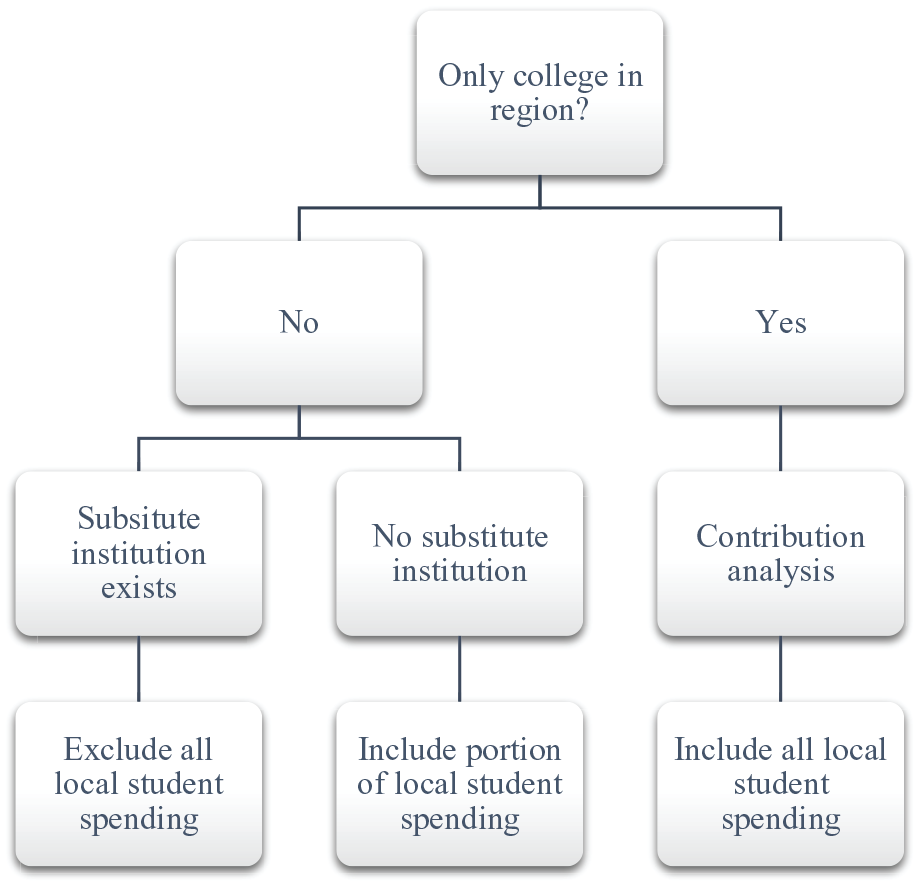
When to include local student spending.
In this article, the focus is economic impact analyses that exclude all local student spending, as these economic impact analyses provide a conservative estimate of regional impact. If the institutions operating in a region are different in nature (e.g., one large state university and one small private college), then the researcher will have to parameterize the model for the share of local student spending to exclude. Local spending from students who would leave the region because of the absence of the institution of interest in search of a similar education setting should still be included in the analysis. This analysis would subsequently require an understanding of local students’ preferences regarding the various types of institutions—an understanding that is impossible to obtain through an analysis of secondary data. It would instead involve the collection of primary data through surveys of local students at the institution under study. Alternatively, the researcher could provide results from an economic contribution analysis, which would include all local student spending as an upper bound of the institution’s regional impact, as well as results from an economic impact analysis that would exclude all local student spending as a lower bound. Adherence to this process therefore circumvents the need for costly data collection.
Study Region and Input Selection
The first critical decision to be made when undertaking an economic impact analysis is in selecting the study region, because this choice is vital in ensuring meaningful results. The region should be large enough to capture the interdependencies among local industries that support the university but small enough that the results are economically significant (Ambargis et al., 2014). For instance, a small liberal arts college may support a large share of the town’s economic activity but a negligible share of the state’s economic activity.
Using a political jurisdiction as the study area often does not allow a regional I-O model to properly account for important interrelationships between economic activities. To give an example, using the county where a university is located will not capture the spending of the university employees who live outside the county or the university spending that occurs outside the county. Core-based statistical areas, such as the U.S. Office of Management and Budget’s MSAs, often serve as good choices for a study region because they consist of areas with close economic ties and encompass regional commuting. However, U.S. Office of Management and Budget designations are less useful in rural areas. Smaller regions may provide insightful results if they contain many of the industries that support the university. A suitable region for a small college should also be a function of the residential location of its employees, and this information is regularly collected by colleges.
Once a decision has been made on the size of the study area, the next step is to determine the inputs, or spending categories, that will be modeled. When examining the various categories of spending analyzed for the economic impact of a university or college, commonalities emerged across studies. Operational expenses of the institution and student spending appeared most often (Blackwell et al., 2002; Carroll & Smith, 2006; Duke University Office of Public Affairs, 2003; Silverstein & Hansen, 2016; Swenson, 2015). Operational expenses of higher education institutions typically refer to a university’s expenditures, such as payroll and tuition dollars from students (Silverstein & Hansen, 2016; Swenson, 2015). Visitor spending is less commonly included because it can be difficult to quantify (Carroll & Smith, 2006; Swenson, 2015). However, as long as the limitations are clear, modeling visitor spending can provide an estimate of the spending that universities attract when holding athletic and nonathletic events (Carroll & Smith, 2006; Duke University Office of Public Affairs, 2003; Silverstein & Hansen, 2016). Construction expenses constitute an additional type of spending that is frequently, though not always, included in economic impact studies (Duke University Office of Public Affairs, 2003; Silverstein & Hansen, 2016). In the following sections, each of these four inputs will be examined in detail.
Operating Impact
First, much of the economic impact of universities and colleges originates from the actual spending of the university. This spending includes all the operations of the college or university as it conducts its business, including personnel costs. An economic impact analysis models a change in the local economy; hence, it is vital that only “new” money coming into the region is modeled (Elliot et al., 1988; Siegfried et al., 2007). As was detailed in the previous section, different elements factor into whether portions of spending from local sources should be included or excluded from an I-O model.
Utilizing university expenses to estimate the economic impact of colleges is the preferred measure of operations, because that approach more closely aligns with how university output is calculated for many institutions in the national I-O accounts (Ambargis et al., 2014). University expenses should include the cost of covering educational services (e.g., instruction and training), student services (e.g., student health clinics and recreational facilities), and other auxiliary operations (e.g., bookstores, residence halls, and cafeterias). However, university expenses should exclude research and development costs, construction, capital purchases, furniture, fixtures, and equipment. Those items are included under capital investments and their impact should be modeled in the corresponding section. Depreciation and interest payments are also excluded to provide a more conservative contribution estimate.
Information on a college’s expenses are available through the college but can also be acquired through the U.S. Department of Education’s Integrated Postsecondary Education Data System (IPEDS) financial survey. The value of university spending, or output, should be adjusted to exclude university services purchased by households in the region, as the impact of their purchases is already captured (Ambargis et al., 2014). Prorating the appropriate measure of university output by the percentage of students that come from outside the region ensures this adjustment.
To illustrate, the researchers employ the IMPLAN economic modeling software version 3.1 and 2017 data sets created by the IMPLAN Group, LLC (Clouse, 2020b). The IMPLAN model generates Social Accounting Matrix (SAM) multipliers, which are then used to calculate indirect and induced effects for each industry. A Type SAM multiplier is calculated by dividing the sum of the direct effects, indirect effects, and induced effects by the direct effects.
The researchers having access to data from Marietta College and Muskingum University, both located in Ohio, as well as IMPLAN data for Ohio, used these two institutions as examples. Marietta is a private, not-for-profit college with 1,130 students and operating expenses equal to $40.7 million in Fiscal Year (FY) 2017. Once depreciation and interest were deducted, the researchers obtained the adjusted operational expenses, which totaled $35 million. This amount needed to be multiplied by the percentage of students from outside the region, equal to 74.8%. This step was performed to exclude university output from purchases by households in the region because local households’ spending would be captured in the total effects through the induced effects. The resulting value was $26.2 million, which was then inputted into IMPLAN to produce an estimate of the college’s contribution to the region. The region used for Marietta College was defined as Washington County, Ohio, and Wood County, West Virginia.
Muskingum University was the other private liberal arts college integral to this study, with 2,848 students enrolled and operating expenses of over $39 million in FY 2019. Once depreciation and interest were deducted, the adjusted operational expenses surpassed $35 million. This amount was then multiplied by the percentage of students who came from outside the region, equal to 71.6%, to again exclude university output from purchases by households in the region. The resulting value was $25.5 million, which was then used as the input in IMPLAN to produce an estimate of Muskingum University’s contribution to the region, defined here as the Ohio counties of Guernsey and Muskingum.
The data used in this article were obtained from Marietta College and Muskingum University directly; this information is easily available for all colleges to access, as institutions are required to report the information annually. The amended Higher Education Act of 1965 requires that institutions participating in federal student aid programs report data on enrollments, program completions, graduation rates, faculty and staff, finances, institutional prices, and student financial aid (National Center for Education Statistics, 2019). However, the students’ counties of origin are not available. Therefore, an economic impact analysis using publicly available data would be limite to a state-level analysis. Through this method, a share of nonlocal students can be proxied using the state of residence of first-time undergraduates, for which information is available through the National Center for Education Statistics.
As shown by Tables 1a and 1b, for each three university or college jobs, an additional job was supported in the regional economy. At Marietta College, its 374 jobs in the universities and colleges industry supported an additional 137 jobs (for a total of 511), producing about $19 million in labor income and over $24 million in regional GDP (e.g., value added). As such, Marietta College contributed about $23 million in added income from operations to the region’s economy in FY 2017, approximately equal to 0.29% of the gross regional product. At Muskingum University, the 353 jobs in the universities and colleges industry supported an additional 129 jobs (a total of 482), generating more than $16.5 million in labor income and more than $21 million in regional GDP. As such, Muskingum University contributed about $21 million in added income from operations to the region’s economy in FY 2019, approximately equal to 0.39% of the gross regional product. Note that the direct employment numbers are estimates from IMPLAN, calculated using the supplied prorated output, and are not a count of direct employment provided by the colleges. Tables 1c and 1d present tax revenue estimates.
Summary of Operation Impact Results for Marietta College (2017).
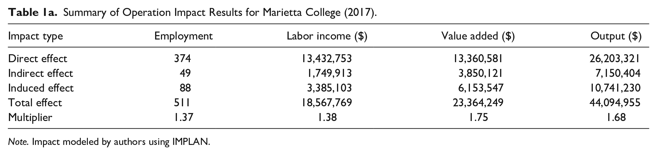
Note. Impact modeled by authors using IMPLAN.
Summary of Operation Impact Results for Muskingum University (2019).
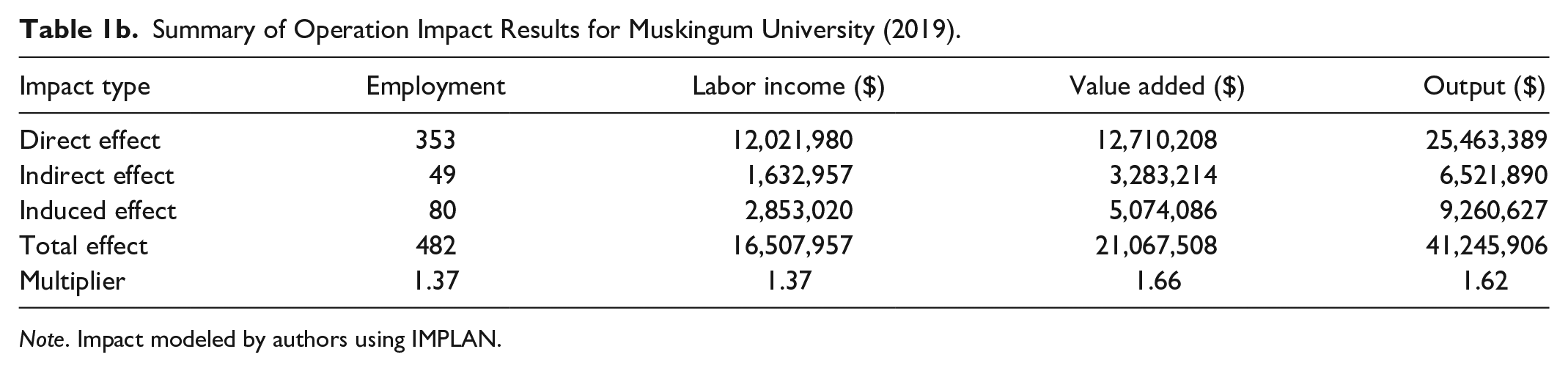
Note. Impact modeled by authors using IMPLAN.
Operation Tax Revenue Results for Marietta College (2017).

Note. Tax revenue modeled by authors using IMPLAN.
Operation Tax Revenue Results for Muskingum University (2019).
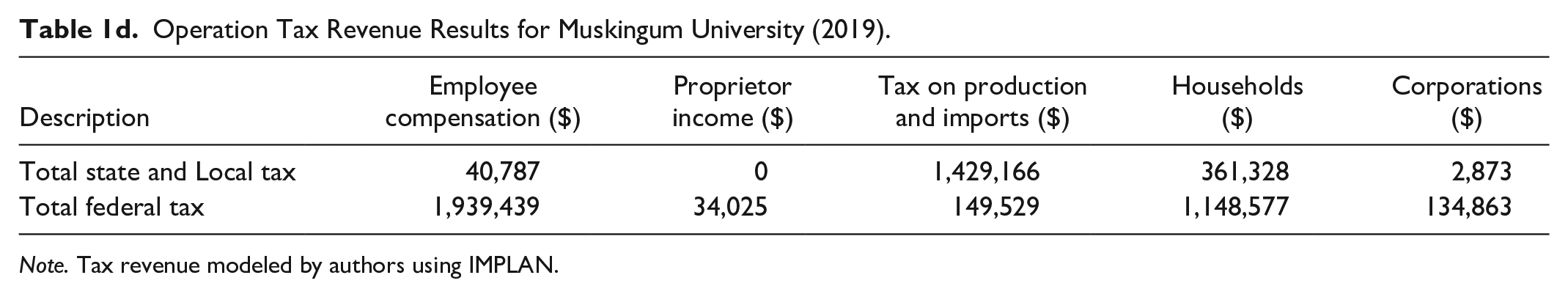
Note. Tax revenue modeled by authors using IMPLAN.
Student Spending Impact
The second type of spending that can be included in economic impact analyses is that of an institution’s students. Student spending includes all spending by students that (a) can be exclusively attributed to the presence of the university and (b) is not already counted in university operations. Student spending includes expenditures of students who have temporarily moved into the region to attend the university, such as off campus housing and groceries at local stores. It does not include tuition or rent paid to the college for on-campus housing, as those expenses are already included in university operations.
Marietta College had 1,130 enrolled students in FY 2017, 74.8% of which originated from counties outside the defined region of analysis. 1 These nonlocal students lived mainly on campus: 698 students resided on campus and 147 resided off campus. Similar to college expenses, information on student residence status (i.e., on campus or off campus) is available to the college but can also be proxied using housing capacity from the IPEDS financial survey. The main difference in modeling student spending patterns for on campus versus off campus students is in their housing costs. The housing cost for students residing on campus is included in the operational expenses of a university; thus, to avoid double counting, it is not included in student spending. Conversely, the housing cost for students residing off campus is included in student spending.
Tables 2a and 2b include spending by student type (i.e., on campus and off campus) for six main spending categories. To avoid double counting, expenses not included when modeling regional impacts are tuition and fees, books and supplies, and housing costs for students residing on campus. For example, if the books and supplies were bought in college bookstores, then they are captured in the operations impact. In contrast, expenditures at restaurants and retail (e.g., grocery stores) or those on gasoline and housing costs for students residing off campus are included when modeling regional impacts of student spending. Student spending patterns for the included expenses are estimated using the Bureau of Labor Statistics Consumer Expenditure survey data for 2016 and 2018 in Tables 2a and 2b, respectively. 2 This resource provides data on the buying habits of American consumers; hence, the data were restricted to survey takers enrolled full time in college who reported living on or off campus. The Consumer Expenditure survey has been used in previous university economic value reports to estimate student spending (Swenson, 2015), but only when providing a conservative estimate of student spending rather than an exhaustive list of expenses. 3
Nonlocal Student Spending for Marietta College (2017).
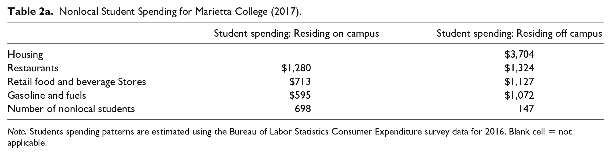
Note. Students spending patterns are estimated using the Bureau of Labor Statistics Consumer Expenditure survey data for 2016. Blank cell = not applicable.
Nonlocal Student Spending for Muskingum University (2019).
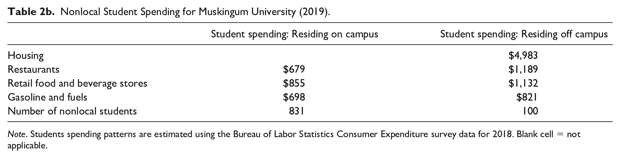
Note. Students spending patterns are estimated using the Bureau of Labor Statistics Consumer Expenditure survey data for 2018. Blank cell = not applicable.
This section estimates the direct, indirect, and induced employment, labor income, value added, and output of student spending on the regional economy. The student spending industries included in the analysis are the full-service restaurants industry (IMPLAN 536 Industry Code: 501), the retail food and beverage stores industry (IMPLAN 536 Industry Code: 400), the retail gasoline stores (IMPLAN 536 Industry Code: 402), and the retail estate industry (IMPLAN 536 Industry Code: 440). As depicted in Tables 3a and 3b, for every four jobs in industries affected by student spending, an additional job was supported in the regional economy. For Marietta College, the 32 jobs from student spending supported an additional 9 jobs (for a total of 41), about $1 million in labor income, and over $1.6 million in regional GDP. For Muskingum University, the 26 jobs from industries affected by student spending supported an additional 7 jobs (or 33 in total), about $723,743 in labor income, and over $1.2 million in regional GDP. Tables 3c and 3d present tax revenue estimates.
Summary of Nonlocal Student Spending Impact Results for Marietta College (2017).
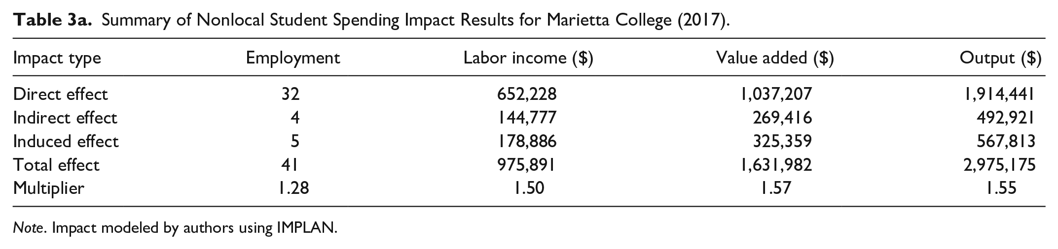
Note. Impact modeled by authors using IMPLAN.
Summary of Nonlocal Student Spending Impact Results for Muskingum University (2019).
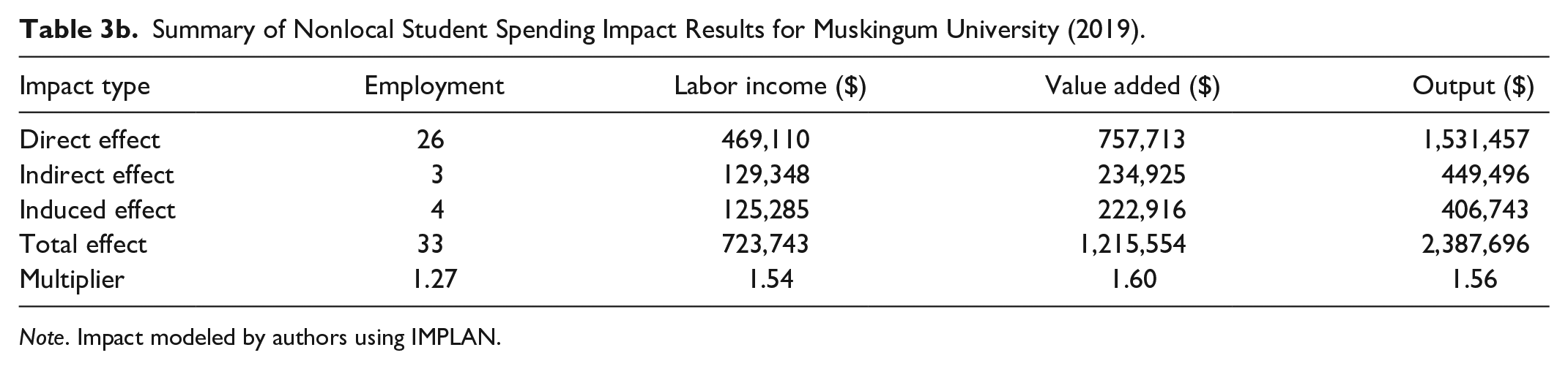
Note. Impact modeled by authors using IMPLAN.
Nonlocal Student Spending Tax Revenue Results for Marietta College (2017).
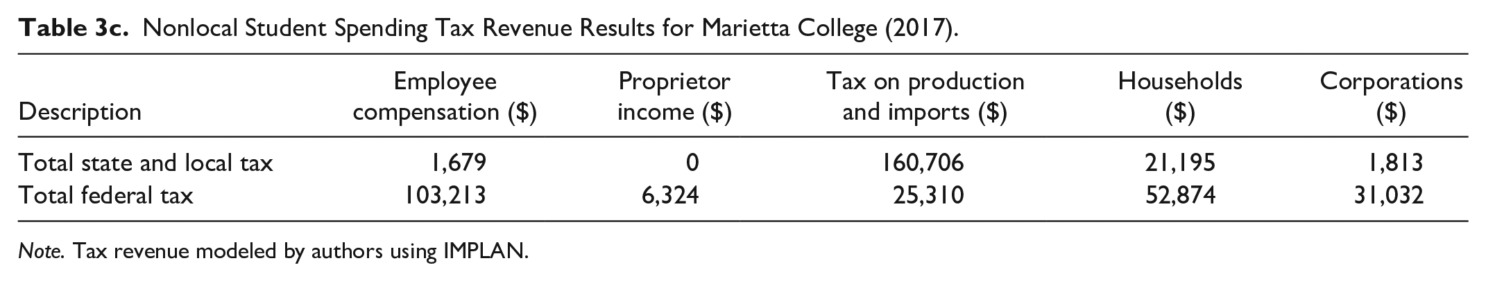
Note. Tax revenue modeled by authors using IMPLAN.
Nonlocal Student Spending Tax Revenue Results for Muskingum University (2019).
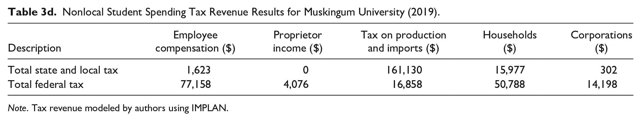
Note. Tax revenue modeled by authors using IMPLAN.
Visitor Spending Impact
The third spending category is from visitors, including prospective students, parents, and arts and sports spectators, among others. Visitor spending includes purchases made by people who visit the region to attend regularly held university events. For long-running or reoccurring events, this economic activity supports local businesses, as visitors stay at local hotels and eat at local restaurants. Lists of campus visitors can be obtained from various universities’ or colleges’ offices and departments that welcome said guests throughout the year. When detailed information on the origin of visitors is not available, the number of visitors should be discounted, similar to university expenses, by the percentage of nonlocal students. Tables 4a and 4b illustrate data provided by Marietta College and Muskingum University, respectively, on the number of visits and events regularly held by the two institutions.
Number of Visitors by Marietta College Event Type (2017).
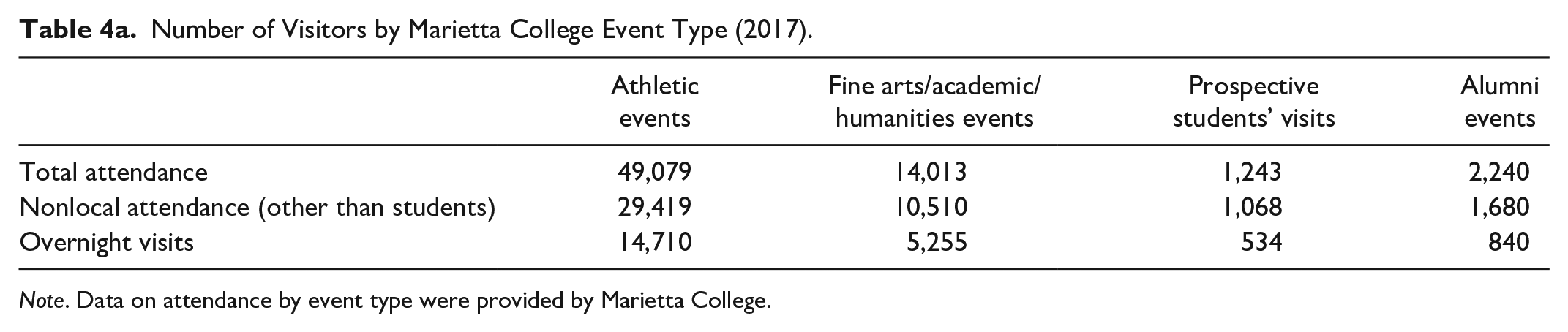
Note. Data on attendance by event type were provided by Marietta College.
Number of Visitors by Muskingum University Event Type (2019).
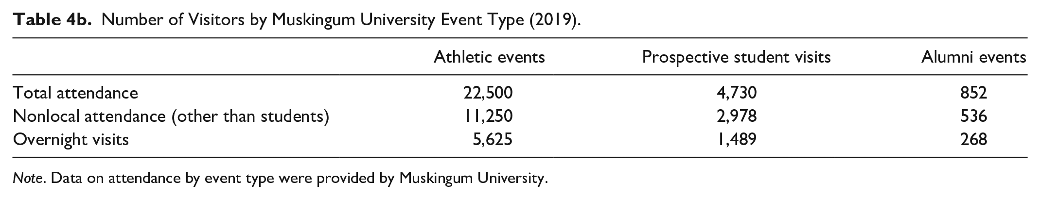
Note. Data on attendance by event type were provided by Muskingum University.
Tables 5a and 5b include visitor spending by spending type. Expenditures were based on data from the U.S. General Services Administration, with the assumption that the private, not-for-profit college is in Ohio. Table 5a includes and categorizes nonlocal visitor spending for Marietta College based on meal-expense and room-rate estimates from 2016. The amount of expenses on meals was estimated at $38.25 dollars per day, 4 while the standard room rate in Ohio was $91 per night. 5 Table 5b includes and categorizes nonlocal visitor spending for Muskingum University based on meal-expense and room-rate estimates from 2019. The amount of expenses on meals was estimated at $41.25 dollars per day, 6 while the standard room rate in Ohio was $94. The estimated average length of stay for overnight visitors was assumed to be 2 days (Alexander et al., 2011; Eslinger, 2016). Additionally, overnight visitors were assumed to constitute 50% of all nonlocal visitors if the number was not provided by Marietta College or Muskingum University.
Nonlocal Visitor Spending for Marietta College (2017).
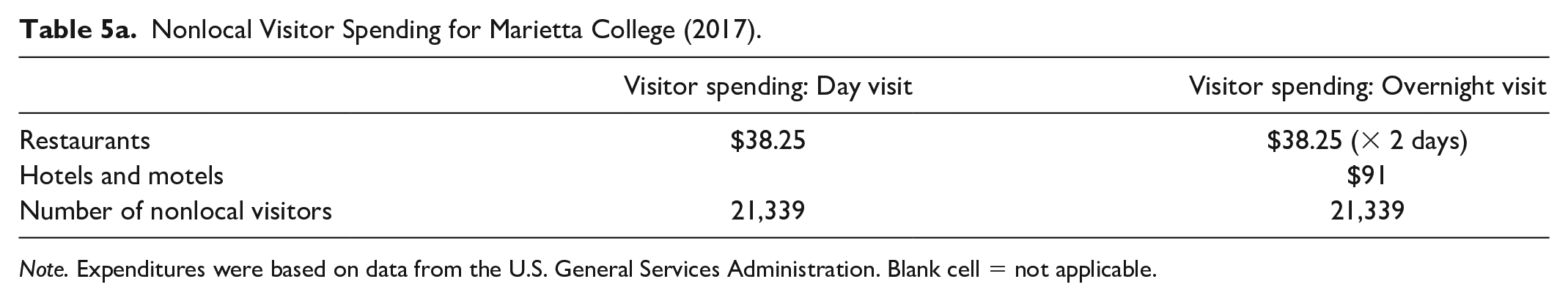
Note. Expenditures were based on data from the U.S. General Services Administration. Blank cell = not applicable.
Nonlocal Visitor Spending for Muskingum University (2019).
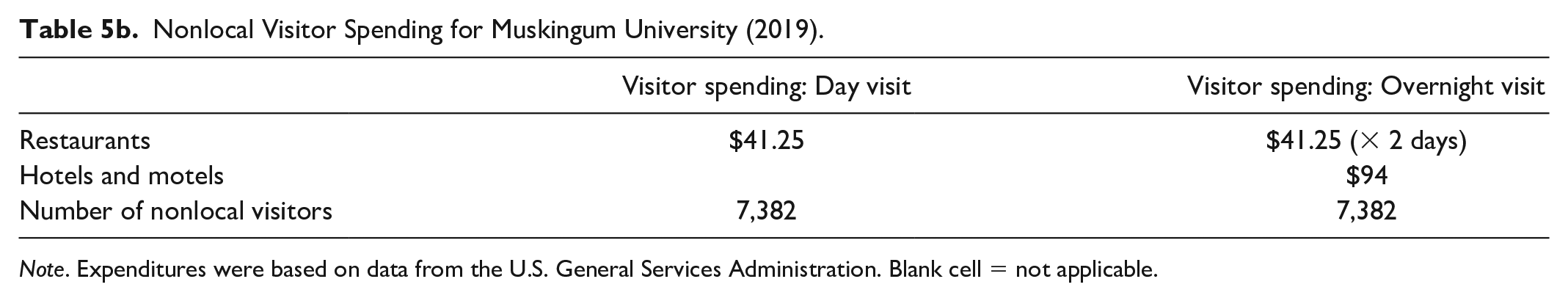
Note. Expenditures were based on data from the U.S. General Services Administration. Blank cell = not applicable.
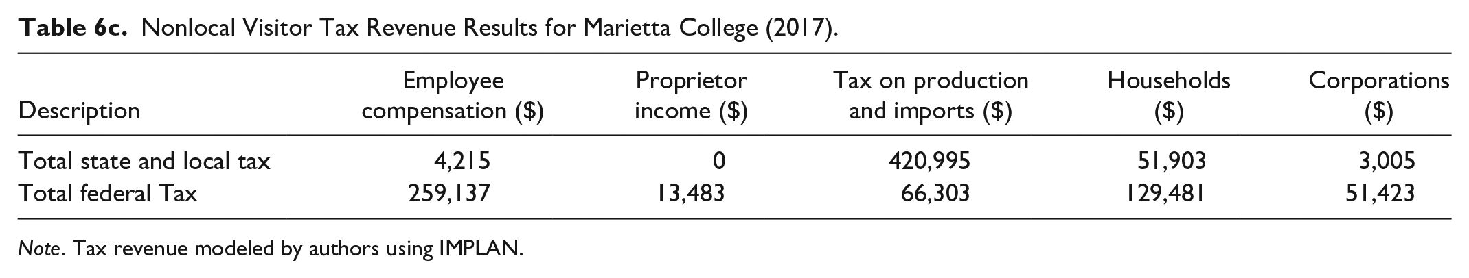
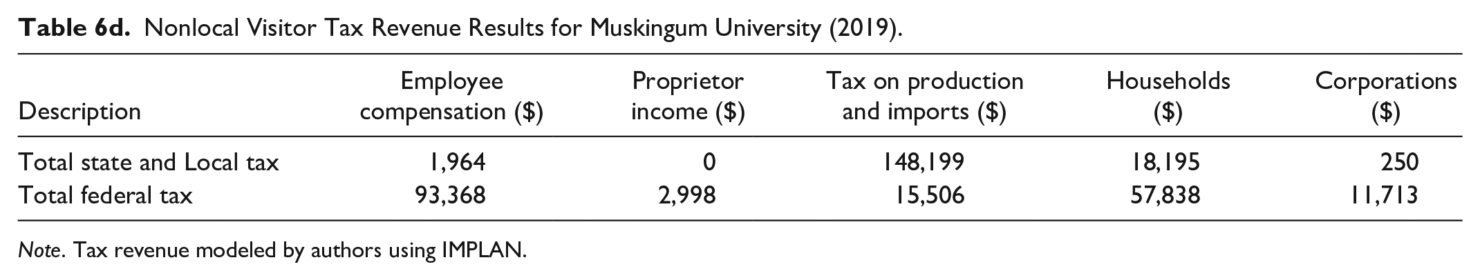
This section estimates the direct, indirect, and induced employment, labor income, value added, and output of visitor spending on the regional economy. The visitor spending industries included in the analysis are the full-service restaurant industry (IMPLAN 536 Industry Code: 501) as well as the hotel and motel—including casino hotels—industry (IMPLAN 536 Industry Code: 499). As shown in Tables 6a and 6b, for each four jobs in visitor spending industries, an additional job was supported in the regional economy. The 74 jobs contributed by Marietta College’s visitor spending industries supported an additional 19 jobs (for 93 in total), about $2.4 million in labor income, over $3.6 million in regional GDP, and $6.9 million in output. In total, Muskingum University visitor spending supported 28 direct jobs (35 total), $828,183 in labor income, over $1.2 million in regional GDP, and $2.5 million in output. Marietta College exhibited larger impacts in absolute terms than those reported by Muskingum College because of the higher attendance across events; nonetheless, we note that the multiplier effect is very similar. Tables 6c and 6d present tax revenue estimates.
Summary of Nonlocal Visitor Impact Results for Marietta College (2017).
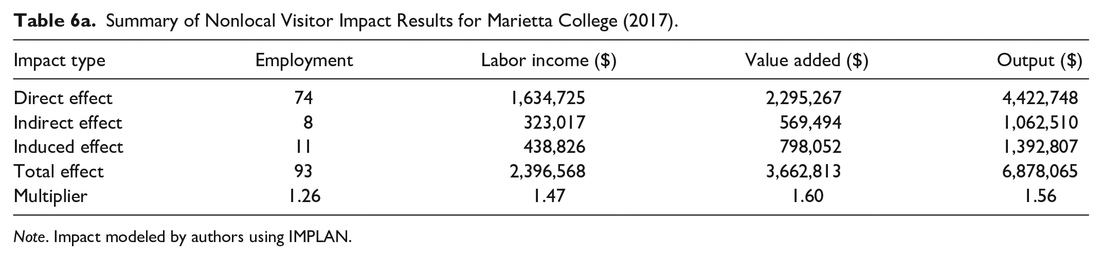
Note. Impact modeled by authors using IMPLAN.
Summary of Nonlocal Visitor Impact Results for Muskingum University (2019).
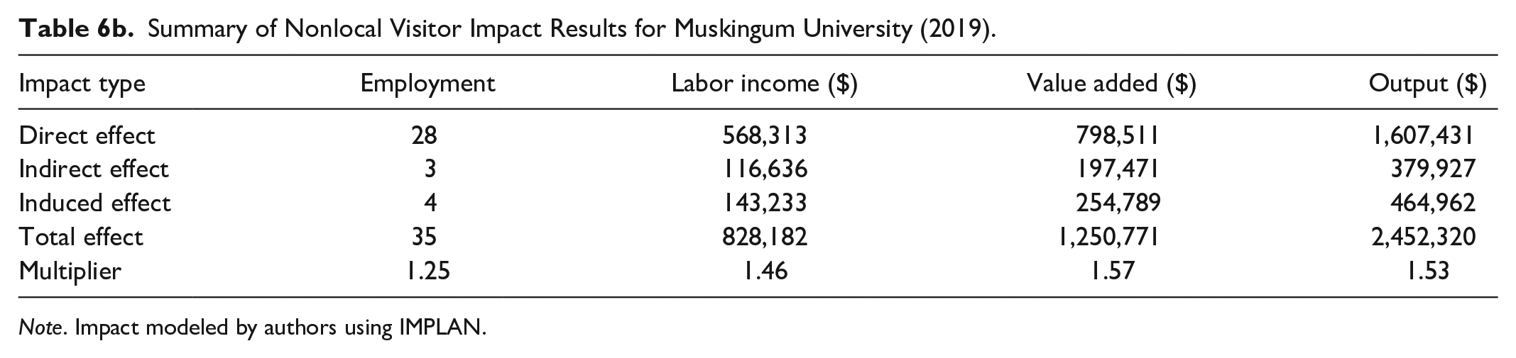
Note. Impact modeled by authors using IMPLAN.
Nonlocal Visitor Tax Revenue Results for Marietta College (2017).
Note. Tax revenue modeled by authors using IMPLAN.
Nonlocal Visitor Tax Revenue Results for Muskingum University (2019).
Note. Tax revenue modeled by authors using IMPLAN.
Construction Impact
Construction and capital spending represent the last impact channel included in this study. Such costs may accumulate over multiple years and can show how a university is using a local workforce and materials in its building projects. Scholars emphasize that investment, business expansion expenditures, and construction of new buildings should be calculated separately, because these changes—not transitional changes to demand—impact final demand (Bess & Ambargis, 2011). To clarify, construction expenses are not an intermediate purchase, such as the purchase of agricultural products used to produce dining services. Instead, these costs represent the production of a final good. As such, they should not be included in the final-demand change that is applied to the multipliers for operations, but rather multiplied by the final-demand multipliers for the construction industry.
This section estimates the direct, indirect, and induced employment, labor income, value added, and output of construction spending on the regional economy. New construction expenses are not treated as part of operating expenses in an I-O model because their impact on the regional economy needs to be calculated separately: construction and capital purchases are one-time purchases, while university operations recur yearly. The construction industry included in this analysis is the construction of new educational and vocational structures industry (IMPLAN 536 Industry Code: 55).
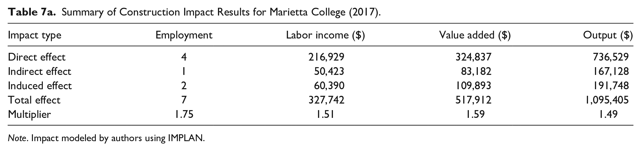
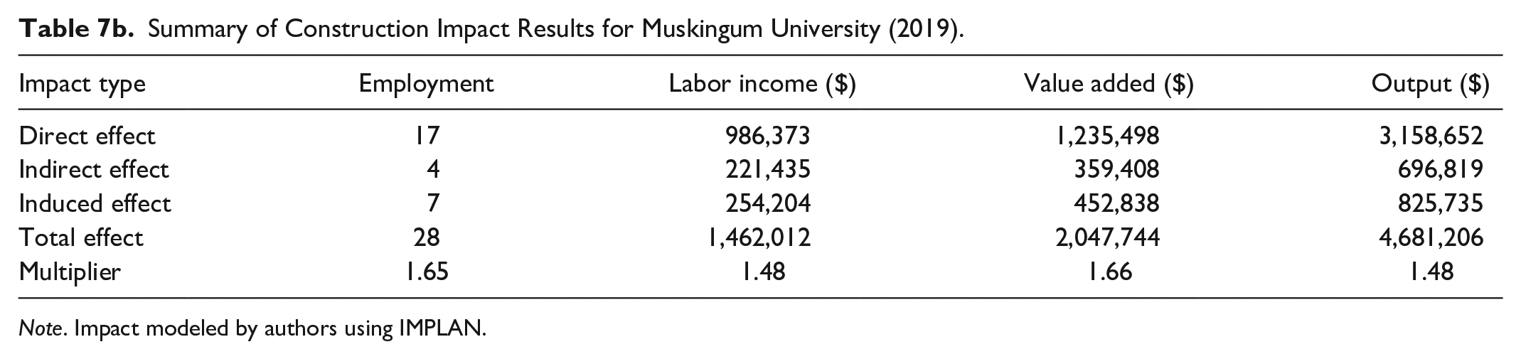
As depicted in Tables 7a and 7b, every two jobs in the construction industry supported an additional job in the regional economy. Marietta College’s contribution of four construction jobs supported an additional three jobs (for a total of seven), more than $300,000 in labor income, more than $500,000 in regional GDP, and just over $1 million in output. In total, Muskingum University’s construction spending supported 17 jobs (28 in total), nearly $1.5 million in labor income, over $2 million in regional GDP, and $4.7 million in output. Again, note that the multipliers are very similar for these two universities. Tables 7c and 7d present tax revenue estimates.
Summary of Construction Impact Results for Marietta College (2017).
Note. Impact modeled by authors using IMPLAN.
Summary of Construction Impact Results for Muskingum University (2019).
Note. Impact modeled by authors using IMPLAN.
Construction Tax Revenue Results for Marietta College (2017).
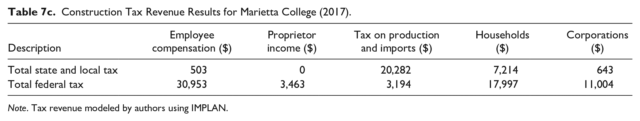
Note. Tax revenue modeled by authors using IMPLAN.
Construction Tax Revenue Results for Muskingum University (2019).
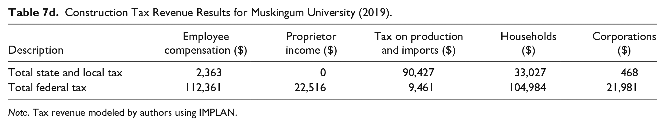
Note. Tax revenue modeled by authors using IMPLAN.
Conclusion and Discussion
An economic impact analysis measures the economic value of a college to its region. This study examines an institution’s impact through the following channels: (a) operating expenses, (b) student spending, (c) visitor spending, and (d) construction expenses. The researchers document best practices and offer a discussion of sources that provide publicly available data that can be used in lieu of expensive surveys to gather information on student and visitor spending.
It is recommended that depreciation and interest payments be excluded from the measure of university output because of the special way these measures are calculated in national I-O accounts (Ambargis et al., 2014). Excluding these two measures results in more conservative contribution estimates. Additionally, the amounts should be prorated to eliminate university output of purchases by households in the region.
Only the spending of nonlocal students is included in this economic impact analysis, using estimates on current spending produced by the Consumer Expenditure Survey. The expenses tallied are not an exhaustive list of all goods and services consumed by students. 7 Furthermore, the conservative estimate provided focuses on the main expenses that do not overlap with operational expenses.
Visitor expenses, modeled here, do not include all possible spending in the region during a visit. 8 The focus is centered on major spending categories, specifically food and lodging. The number of visits and the portion of overnight visits can be provided by the college under study. Important to note is that the amount spent by visitors varies tremendously by the type of activity attended (Swenson, 2015); therefore, the estimated visitor spending impact should be interpreted with caution. Construction expenses included in an analysis can also be provided by the college.
For Marietta College, the direct economic benefit to the college in FY 2017, including all university operations, student spending, visitor spending, and construction activity, was an estimated $33.3 million in output, as seen in Table 8a. Through the multiplier effects of this direct spending, the college supported an additional $21.8 million of output in all industries throughout the region. In total, Marietta College contributed over $55 million in output to the region in FY 2017. The direct economic benefit of Muskingum University, including all university operations, student spending, visitor spending, and construction activity, was an estimated $31.8 million in output in FY 2019, as seen in Table 8b. Through the multiplier effects of this direct spending, Muskingum University supported an additional $19 million of output in all industries in the region. In total, Muskingum University contributed almost $51 million in output to the region in FY 2019.
Total Impact of Marietta College (2017).
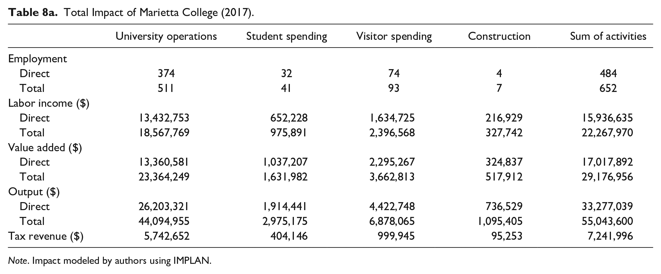
Note. Impact modeled by authors using IMPLAN.
Total Impact of Muskingum University (2019).
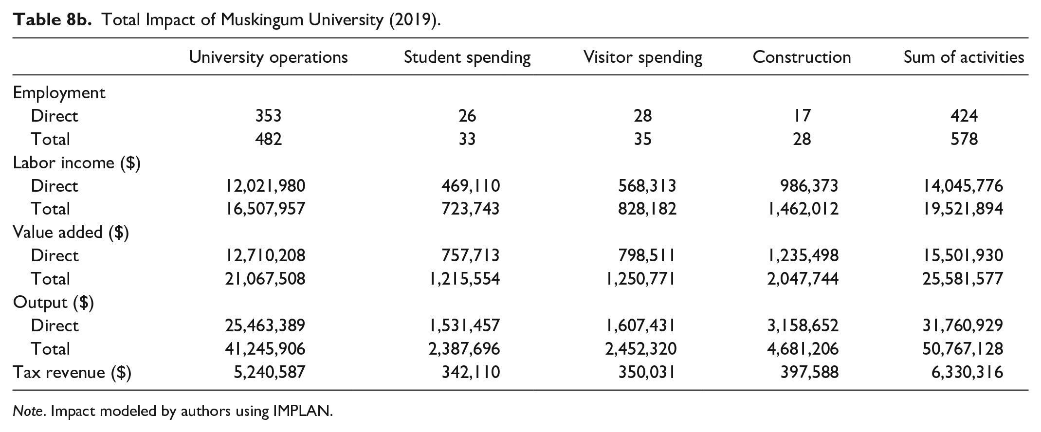
Note. Impact modeled by authors using IMPLAN.
Note that total output estimate provides the largest impact in dollar terms in these studies, and also provides the greatest marketing benefit for colleges and universities to report out. However, most academic studies focus on employment and value added as more important indicators (e.g., Jolley et al., 2020). In the case of colleges and universities, employment demonstrates the anchor institution effect of these organizations as leading employers, and value added, while a smaller number than total output, represents their contribution to the regional GDP.
The estimated impacts provided offer a conservative look at both colleges’ contributions to their regions, for these institutions have other economic development benefits not quantified here. For example, a college’s presence provides educational opportunities and attracts talent to the region. There is an economic benefit to raising the income of residents through educational advancement and increasing the future income stream maintained by graduates who stay to work in the area (Beck et al., 1995). However, leveraging college graduates as drivers of innovation and economic development hinges on the ability of localities to retain these graduates. Identifying the determinants of retention is a complicated process, but some evidence suggests that most small colleges and universities, especially those in metro areas, are likely to retain a large percentage of locals and students from outside the region who were educated at the college (Florida, 2016). While benefits likely accrue to the college town or region when graduates remain in the area postgraduation, it must be acknowledged that the benefits to the graduates may not be as favorable. Winters (2012) studied 41 U.S. metropolitan areas that were classified as college towns. He found that college graduates who stayed in the college metro area where they had earned their degree earned lower wages and worked in “less educated occupations” that their counterparts who had relocated to other areas (p. 1).
Additional benefits not quantified here include academic entrepreneurship, defined as spin-off activities of the college that contribute to firm formation, university–industry collaboration, local and regional spillover effects on local innovation, production, and other aspects of the value chain (Bagchi-Sen & Smith 2012). Some of the body of applied work in this area has been generated by the Association of Public and Land Grant Universities and the University Economic Development Association, which brought together 50 higher education leaders for input to produce Higher Education Engagement in Economic Development: Foundations of Strategy and Practice in 2015 (Klein & Woodell, 2015). Follow-on work by Talebzadehhosseini et al. (2019) further classified the application of this work into six areas of economic engagement typology, including both promoting the transfer of new technologies to industry and encouraging entrepreneurial activities. While application of this typology to university activity has been applied by scholars to a regional university (Jolley & Michaud, 2019), the suite of activities rests largely with land grant and large public universities. Consistent with this, most work on entrepreneurial ecosystems has focused on established ecosystems in urban areas, and there has been limited focus on entrepreneurial ecosystems in various stages of development in smaller cities or college towns (Jolley & Pittaway, 2019). While some metrics, such as tech transfer and university patents, are lower or nonexistent at smaller colleges and universities, these institutions remain important existing or potential sources of entrepreneurial training beyond the traditional academic classroom, especially in rural or underserved areas (Lyons et al., 2019a, 2019b). Furthermore, the mere presence of a university in a region has a positive effect on the location decisions of firms and individuals, as it can enhance the “amenities” value of a community or region.
Footnotes
Declaration of Conflicting Interests
The author(s) declared no potential conflicts of interest with respect to the research, authorship, and/or publication of this article.
Funding
The author(s) received no financial support for the research, authorship, and/or publication of this article.