
Abstract
This study makes three contributions to the debate over the effect of local land use regulations on housing prices and affordability. First, it is more geographically extensive than previous studies, encompassing 336 of the nation's 384 metropolitan areas. Second, it looks at multiple measures of regulatory stringency, not just one. Most prior studies have focused either on a single regulatory measure or index across multiple metropolitan areas, or multiple regulatory measures in a single region. Third, this paper considers the connection between regulatory stringency and housing values as a function of employment growth and per-worker payroll levels. We find that restrictive land use regulations do indeed have a pervasive effect on local home values and rents, and that these effects are magnified in faster-growing and more prosperous economies. We also find more restrictive land use regulations are not associated with faster rates of recent home value or rent growth, and that their effects on housing construction levels—that is, the degree to which they constrain supply—is uneven among different housing markets.
Developers, economists, and many housing policy makers have made the case for years that excessive land use regulations have inflated housing construction costs, restricted residential densities, and reduced housing construction in a manner that needlessly raises housing prices and rents (see, e.g., Advisory Commission on Regulatory Barriers to Affordable Housing, 1991; Dowall, 1984; Fischel, 2001; Freeman & Schuetz, 2017; Frieden, 1979; Glaeser et al., 2005; Pollakowski & Wachter, 1990; Quigley & Raphael, 2004; Quigley & Rosenthal, 2005; Schuetz, 2009; Siegan, 1972). Such price increases, when coupled with stagnant or slow-growing household incomes, have translated into severe affordability hardships, particularly in expensive coastal markets, and especially for low- and moderate-income renters (Joint Center for Housing Studies, 2019; Landis & Reina, 2019). The possibility of rolling back local zoning and land use regulations has been raised anew in recent years, whether as a means of moderating sky-high housing prices in high tech economies (Dougherty, 2020) or as a vehicle for increasing infill and multifamily housing construction (Monkkonen, 2019).
This paper clarifies these arguments by examining the associations between land use regulations and housing costs and prices across the fullest set of U.S. metropolitan areas for which reliable data are available. In doing so, it offers three original contributions. First, it is more geographically extensive than any previous study, encompassing 336 of the nation's 384 metropolitan areas. 1 So far, most empirical studies of the housing-price land-use regulation connection have been limited to a few highly regulated and visible markets like San Francisco, New York City, or Seattle; this paper fills out the map. Second, this paper looks at multiple measures of regulatory stringency, not just one. Most prior studies have focused either on a single regulatory measure or index across multiple metropolitan areas, or multiple regulatory measures in a single region. This paper looks at multiple measures in multiple places. Last, this paper considers the connection between regulatory stringency and housing values as a function of local economic growth. Theory suggests that the inflationary effects of local land use regulations should be greater in places where a booming economy is driving an increased demand for housing than in lagging economies with little job or income growth. Are these expectations born out in fact?
As measured at the metropolitan scale, we find that restrictive land use regulations do indeed have a pervasive effect on local home values and rents, and that these effects are magnified in faster growing and more prosperous economies. We also find more restrictive land use regulations not to be associated with faster rates of recent home value or rent growth, and that their effects on housing construction levels—that is, the degree to which they constrain supply—to be extremely uneven among different housing markets.
The remainder of this paper is organized into five sections. The section titled “Literature Review” briefly reviews the empirical literature connecting residential land use restrictions and housing market outcomes. The section “Data and Methods” provides an overview of the data and methods used in this paper and explains the different schemas used to measure regulatory stringency. The “Regression Results” section summarizes our statistical modeling results, and section “A Closer Look At Local Land Use Regulations and Housing Affordability” looks at whether relaxing overly stringent land use regulation would help make housing more affordable. The section “Conclusions and Policy Recommendations” summarizes the main findings and presents a series of policy recommendations for reducing the adverse housing price effects of poorly targeted residential land use regulations.
Literature Review
Free-market-oriented economists and real estate interests have complained about the adverse housing cost and affordability impacts of local land use and building regulations for more than 100 years. In the 1890s, New York City tenement builders pushed back against the minimal health and safety regulations being proposed arguing that they would make housing unaffordable to the hundreds of European immigrant families arriving daily (Lubove, 1963). Thirty years later, Florida bankers and land speculators organized to protest the adoption of regulations designed to outlaw fraudulent land subdivisions, claiming that such regulations were contrary to America's free enterprise system (Vickers, 1994). With housing production going full steam in the 1960s, the argument over excessive government regulation shifted from land development to local building codes, which, it was argued, were stifling labor and cost-saving innovations (Noam, 1982). The first mention of the potential supply-constraining effects of single-family zoning—it had long been criticized as being racially and economically exclusionary (Pendall, 2000; Reina et al., 2021; Rothstein, 2017; Rothwell & Massey, 2009)—came from legal scholar Bernard Siegan, who in his 1972 book, Land Use Without Zoning, pointed out how Houston's lack of zoning enabled its homebuilders to deliver more new homes at a lower cost than anywhere else in the country. Siegan's critique of zoning was followed up in 1979 by The Environmental Protection Hustle, a similarly critical assessment of local environmental regulations in California's Marin County by Bernard Frieden. Instead of protecting the natural environment, Frieden argued, such regulations mostly functioned to restrict construction, thereby driving up the property values of already well-off homeowners.
In theory, overly stringent land use regulations affect housing and real estate prices in three ways (Dowall, 1984). First, they add to the costs of land development and construction, with the increase in costs ultimately passed on to the homebuyer or renter. Second, they restrict new construction, which, in the presence of strong or consistent demand, will add to prices. Third, they restrict the number of developers to those with the most capital and knowledge of the process, decreasing the supply of builders.
Few empirical studies consider these dynamics explicitly. Instead, most compare the presence of land use regulations in a particular community or metro area to housing prices and/or rents. This can be done on an individual property level by comparing the prices of regulation-affected and unaffected properties, or it can be done at a community level by comparing average (or median) prices between affected and unaffected communities. Depending on the study, the extent and stringency of local regulations are measured as one or more fixed effect variables indicating the presence or absence of particular programs, and/or as a constructed index of regulatory stringency based on tabulations of local growth management (LGM) programs or surveys of local planners. In most cases, regression analysis is used to statistically control for the effects of relevant nonregulatory variables such as house size or distance to the city center. Table 1 summarizes many of the more notable property price studies and their findings.
Property Price Effects of Local Land Use Regulation Programs: Summary of Selected Empirical Studies.
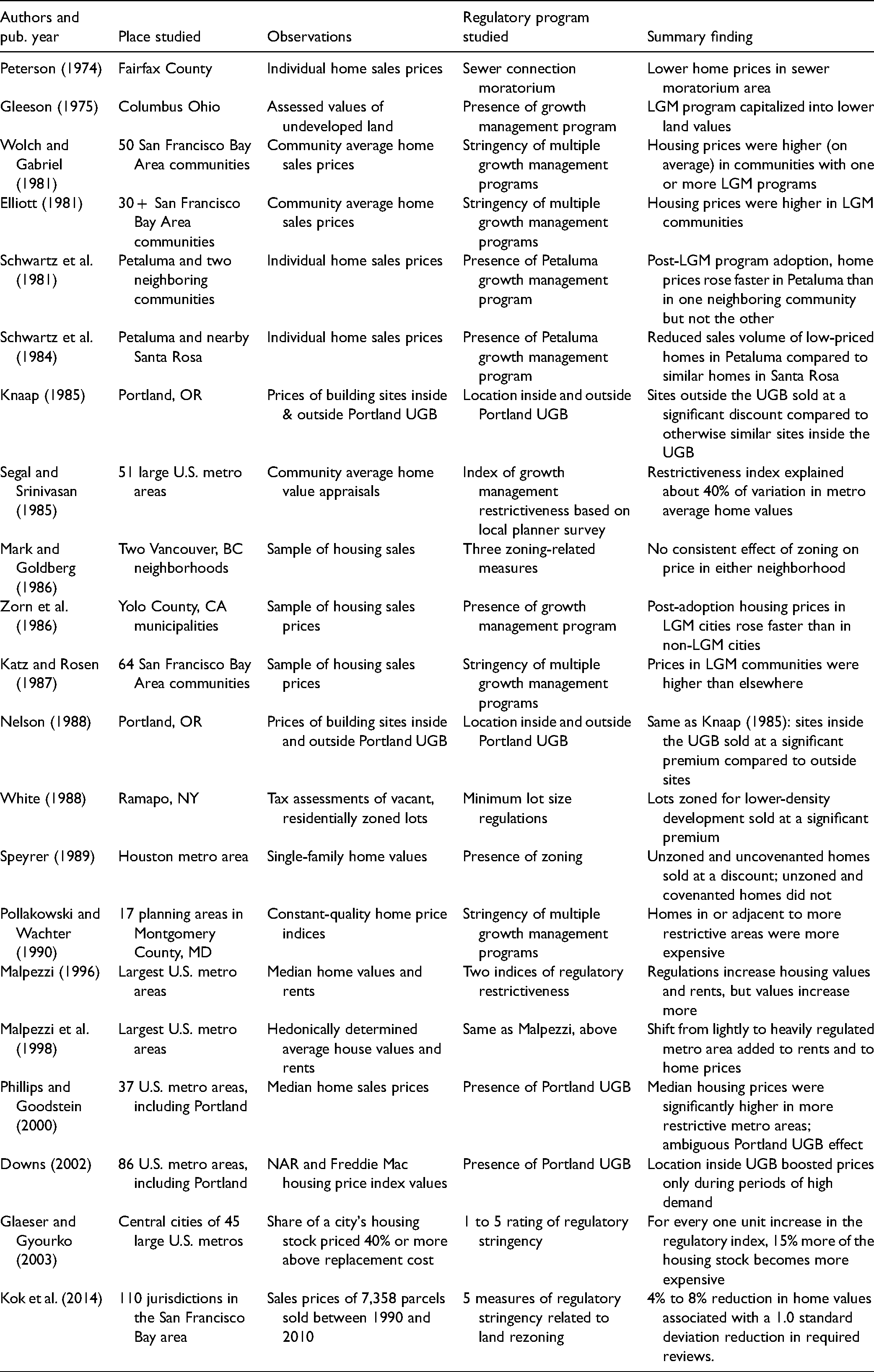
Examples of individual property studies include Peterson (1974), Schwartz et al. (1981, 1984), Knaap (1985), Mark and Goldberg (1986), Zorn et al. (1986), Katz and Rosen (1987), White (1988), and Speyrer (1989). Examples of community average price studies include Wolch and Gabriel (1981), Elliott (1981), Dowall and Landis (1982), Segal and Srinivasan (1985), Pollakowski and Wachter (1990), Malpezzi (1996), Phillips and Goodstein (2000), Downs (2002), and Glaeser and Gyourko (2003). Each study is set in a different period, and because most do not control for the macroeconomic conditions of their day—especially the effects of mortgage interest rates—the results are rarely comparable across studies. Depending on the community, period, and approach to measuring regulatory stringency, these studies produce estimates of the effects of local land use regulations on housing prices ranging from 5% to 20%. As expected, adverse price effects were found to be greater when adjacent communities all adopted similar restrictive regulations.
Most of these studies are best characterized as “after effect only,” meaning that they measure the effects of regulatory programs on home prices and land values only after those programs are in place. A more robust approach would be to use a difference-in-differences design, comparing home prices before and after the imposition of a particular regulatory program as well as between regulated and unregulated communities. This was the approach taken by Zorn et al. (1986) in their analysis of constant-quality home price changes in Yolo County, California between 1971 and 1979, in which they observed that homes sold in Davis (the only highly regulated community in Yolo County at the time) after the imposition of a new growth management program sold at an 8% premium compared to homes sold before the program was implemented.
As the adoption of state and LGM programs in fast-growing states like California and Florida accelerated during the 1980s (Bollens, 1992), it became more difficult to find unregulated communities to compare with nearby regulated ones. This prompted some researchers to shift their focus to the metropolitan level. Among the first to do so was Malpezzi, who, in a 1996 study, compared median home values and rents among the 58 largest U.S. metro areas to two different metro-level indices of regulatory restrictiveness. Shifting from a lightly to heavily regulated metro area, Malpezzi found, accounted for 51% of the intermetropolitan area difference in median home prices. 2 Subsequent work by Malpezzi et al. (1998), using a more robust measure of housing quality and prices, found that a similar least-to-most shift in local regulatory practices was associated with a 9% to 15% increase in rents and a 30% to 45% increase in constant-quality home values.
The falling mortgage rate and lax lending environment of the late 1990s and early 2000s caused housing prices to rise almost everywhere in the United States, making it difficult to isolate the effects of community-level land use regulations. Prices rose tremendously in housing supply-constrained markets like New York City, Boston, and San Francisco, but they also rose in less-constrained markets like Phoenix, Tampa, and Las Vegas. Empirically disentangling the price effects of local regulations and regional supply constraints from shifting demand-side preferences and price speculation became an empirically fraught proposition. Instead of comparing housing prices across metro areas, Glaeser and Gyourko (2003) compared the difference between housing price levels and physical replacement costs, presuming that construction costs should be less affected by local regulations. The authors found that for every one-point increase on their 1-to-5 regulation scale, average housing prices would rise another 15% compared to local replacement costs.
Planners and economists were also becoming increasingly aware that the housing price effects of local land use regulations are cumulative and may vary widely according to the stringency with which they are implemented (Landis, 1992, 2006). In a study comparing regulatory stringency, land values, and housing values among San Francisco Bay municipalities, Kok et al. (2014) found both land and housing prices to be higher in cities requiring that projects undergo additional regulatory reviews to obtain a needed building permit or zoning change. Taking a comparable approach at the national level, Gyourko et al. (2008) developed a detailed survey of residential regulatory practices that they mailed to more than 2,600 municipalities nationwide. Using factor analysis, they combined the survey responses into 11 regulatory subindices, and combined them again into a single, composite index they called the Wharton Residential Land Use Regulatory Index, or WRLURI. The WRLURI measure has since been used in studies exploring housing supply elasticities (Saiz, 2010) and the equity impacts of local land use regulations (Lens & Monkkonen, 2016), but curiously, not the housing price or rent effects. In a dissenting note, a recent review of survey-based regulatory measures like WRLURI calls into question their accuracy measuring regulatory stringency (Lewis & Marantz, 2019).
More recently, researchers have focused on the potentially negative effects of land use regulations on regional job growth and economic output (Glaeser et al., 2005; Hsieh & Moretti, 2015, 2019; Saks, 2005). The first part of their argument is simple and intuitively appealing: Rather than pay the higher salaries required for their employees to live in housing supply-constrained metro areas like San Francisco or Seattle, major national employers will choose to expand in lower-cost markets like Phoenix or Atlanta. Likewise, instead of using precious start-up capital to pay San Francisco or Seattle's inflated housing costs, would-be entrepreneurs will relocate to less expensive job markets where they can grow faster and add more new jobs.
The second part of this argument is more complicated and contentious: Because worker productivity in some types of industries may be higher in San Francisco (for example) than in Phoenix, had the same employees originally gone to San Francisco (or started new businesses there), aggregate economic activity would have increased by a greater amount. What excessive land use restrictions do, in this view, is shift valuable investment capital from potentially productive functions like new business and job creation directly into the pockets of existing property owners in the form of unearned rents. This represents a loss not only to the residents and businesses of cities like San Francisco, but to the national economy as whole.
Data and Methods
This section introduces the various measurement schemas used to construct a series of linear regression models relating median home values and rents to land use regulatory regimes, regional economic and labor market conditions, and community amenities as measured at the metropolitan level. The results of these regressions are presented in the next section.
Using metropolitan areas as the unit of analysis rather than individual municipalities has its pros and cons. On the positive side, metropolitan areas reasonably approximate housing and labor markets in terms of their size and extent so the problem of ecological fallacy is reduced. 3 In addition, all the variables of interest vary widely among metropolitan areas. To the degree that the models fit the data well, the resulting associations are likely to be robust. On the negative side, most metropolitan areas are internally diverse in terms of their regulatory regimes, housing and labor market conditions, and socioeconomic characteristics and amenities. This means that regression model results, while indicative for metro areas as a whole, may not apply with equal validity among communities and neighborhoods within metropolitan areas. Thus, it may be that a particular regulatory measure has no effect on median home values and rents when measured at the metropolitan scale but has a notable effect when comparing communities within a single metro area. With these caveats in mind, we turn to the question of how to accurately and reliably measure local land- use regulations at the metropolitan scale.
Measuring Regulatory Stringency and Housing Supply Flows at the Metropolitan Level
There have been three notable efforts during the last 20 years to survey and catalog local land use regulations at the metropolitan and national scales. The first was a study conducted by the Brookings Institution based on the results of a 2003 survey of local land use regulations in 1,844 jurisdictions in the 50 largest U.S. metropolitan areas (Puentes et al., 2006). A second survey of local land use regulations was undertaken in 2005 by researchers at the University of Pennsylvania (Gyourko et al., 2008). Referenced earlier as the Wharton Regulatory Land Use Restrictiveness Index, it reports on the restrictiveness of residential land use regulations in 2,700 municipalities 4 across all 50 states as of 2006. (The original Wharton survey was updated in 2018 [Gyourko et al., 2019] but with fewer observations.) The results of a third national survey of local land use regulations were published online in database form in 2019 by The Urban Institute. 5 The Urban Institute's database builds on prior 1994 and 2003 surveys by Pendall et al. (2018); like the earlier Brookings study, is limited to the country's 50 largest metropolitan areas.
Each of the three studies approached their task in different ways. The Brookings study resulted in a typology that classified each metropolitan area as conforming to one of four regulatory regime categories: (1) Traditional regulatory regimes, which rely on local zoning as their principal regulatory tool; (2) Exclusionary regimes, which make it intentionally difficult for developers and builders to up-zone single-family parcels to apartment use; (3) Reform regimes, in which local comprehensive plans and various growth management programs (e.g., building permit caps, urban containment schemes, infrastructure limitation provisions) are used together with zoning to regulate development; and (4) Wild West Texas regimes in which zoning ordinances and comprehensive plans, if adopted at all, are administered in a manner that is more advisory than binding. 6 The popularity of each regime varies regionally. Traditional regimes are prevalent in Mid-Atlantic and Midwestern metropolitan areas. Exclusionary regimes are more common in metropolitan areas in New Jersey, Massachusetts, and Maryland. Reform regimes predominate among western states as well as metro areas in Florida and Tennessee. Wild West Texas regimes are found only among metropolitan areas in Texas.
Rather than produce a typology, the University of Pennsylvania-Wharton study calculates a single index value of residential land use restrictiveness for each state and many major metropolitan areas. The index is calculated using factor analysis to combine survey results in 11 regulatory areas, including (1) local stakeholder involvement in regulating residential land uses; (2) state government involvement in local development issues; (3) state court involvement in local development conflicts; (4) the number of entities required to approve residential rezoning; (5) the type and number of nonzoning approval requirements; (6) the number and type of required public comment meetings; (7) the presence of zoning or building permit caps; (8) the existence of a 1-acre minimum residential lot size category; (9) the presence of an open space set-aside requirement; (10) the presence of residential exaction or infrastructure requirements; and (11) the duration of the residential approvals process. Positive values of the WRLURI indicate that a state or metropolitan area is more restrictive than the national average; negative values indicate that a state or metropolitan area is less restrictive than average. For states, WRLURI values range from a high of 2.34 for Hawaii to a low of −1.11 for Kansas. Among the 47 metro areas for which WRLURI values were calculated, values range from a high of 1.76 for the Providence-Fall River-Warwick metro area to a low of −.79 for the Kansas City metro area.
The Urban Institute's 2019 survey results (Gallagher et al., 2019) are available online as part of the National Longitudinal Land Use Survey, or NLLUS. So far, they exist only as frequencies and cross-tabulations, and have not yet been used to develop summary typologies or indices.
Based mostly around zoning, none of the three schemas fully captures the diversity of tools available to local governments to regulate private development. Precisely for this reason, we developed a second index to measure the regulatory intensity of local development control processes as set forth in state planning and redevelopment laws. Ranging in value from 0 to 8, the Beyond Zoning Regulatory Intensity Index (BZRII) adds the number of times state planning laws give local governments one of six specific planning powers or regulatory responsibilities beyond zoning. The six include (1) whether local governments are required to prepare comprehensive plans covering land use, housing, and transportation; (2) whether local zoning ordinances must be consistent with local comprehensive plans; (3) whether private development projects must be subjected to state and/or local environmental reviews; (4) whether local annexations are subject to legislative or quasijudicial review; (5) whether state law allows local tax increment financing (TIF) or redevelopment districts to use eminent domain to acquire land for private development; and, (6) whether TIF or redevelopment districts can be established without a majority vote of the affected land holders. These tabulations were derived from Meck (2002).
States are given scores of either 0 (indicating that local governments in that state do not have such powers) or 1 (indicating that they do) in each of the six categories. States that require local comprehensive plans to include specific housing and land use goals are given a comprehensive planning category score of 2 instead of a 1. California metro areas automatically earn a score of 2 in the environmental review category because the California Environmental Quality Act (CEQA) leaves the determination of impact assessment criteria to each local government rather than establishing them at the state level. When the individual category scores are added, one state, California, earns a total BZRII score of 7 out of a maximum score of 8. Another state, Washington, earns a total score of 5. Five states earn total scores of 5; eight states earn a total score of 4; 13 states earn a score of 3; 18 states earn a score of 2; four states earn a 1; and one state, Kansas, earns a total score of 0. The average BZRII for all 50 states is a relatively modest 2.8. Online Appendix A lists each category score by state.
How do the WRLURI and BZRII measures differ? As an analogy, consider the differences between amperage and voltage as measures of electric current. Voltage is a measure of the pressure that allows electrons to flow, while amperage is a measure of the volume of electrons. The BZRII is like voltage: it is a measure of the power local regulators is given by state law to push back against development projects they regard as objectionable. The WRLURI is like amperage: it is a measure of the variety of stakeholders—including local legislative bodies, the courts, community groups, and regulators—and regulation that may affect a given residential development outcome.
The WRLURI and BZRII both measure how the local regulatory process is organized. They don’t measure its outcomes—the degree to which regulations limit residential supplies. For this, we make use of the knowledge that housing demand, as measured at the metropolitan scale, is principally a function of job and wage growth (Glaeser et al., 2006; Glaeser & Shapiro, 2001; Landis et al., 2002). Job growth is a metric for demand because newly arriving workers and their families necessarily need a place to live, and wage growth is another because one of the first things workers who receive a raise do is re-evaluate their housing situations.
By coupling annual U.S. Census Bureau housing estimates with nonfarm employment data from the U.S. Bureau of Labor Statistics, we can compare the degree to which homebuilders in every metropolitan area have been able to keep production on pace with job growth. Nationwide, the ratio of housing unit change to job change (a measure we will henceforth abbreviate as the HUC-JC-ratio) between 2000 and 2018 stood at 1.14. This means that 114 new housing units were produced for every 100 new jobs. Some amount of inter- and intrametropolitan variation around this average is to be expected because of differences in vacancy rates, the number of workers per household, and the popularity of second or vacation homes. For the most part, however, we should expect state and metropolitan HUC-JC-ratios to not depart too far from the national average.
It is therefore something of a surprise to observe 2000 through 2018 HUC-JC-ratios varying among states from a high of 6.3 in Connecticut (meaning that 6.3 new homes were built in Connecticut between 2000 and 2018 for every new job) to a low of just 0.4 in neighboring New York. Among the 235 metro areas that gained both jobs and dwelling units between 2005 and 2016, 7 HUC-JC-ratios ranged from a low of just 0.08 in Pittsburgh, Pennsylvania to a high of 48.3 for Jefferson City, Missouri. To the degree that local HUC-JC-ratios fall far below the national average, especially in rapidly growing economies, we may surmise that some set of conditions or constraints are preventing local homebuilders from responding to demand. More often than not, the culprit is likely to be excessive land use and housing regulations.
To avoid overspecifying our home value and rent regressions, we first needed to ensure that the various regulatory stringency indicators are not measuring the same effects. Table 2 presents a correlation matrix comparing Brookings’ typology values, WRLURI values, BZRII values, and 2000 to 2018 HUC-JC-ratios across all the metropolitan areas included in this study. Since laws regulating development are mostly determined at the state level, metro-level BZRII values are based on their state-level values. Using the methodology explained in (online) Appendix B, updated WRLURI values (WRLURI-R) were calculated for metro areas not included in the original Wharton study. Brookings regulatory regime categories were first assigned upward to states based on their metropolitan areas, and then downward to additional metro areas within each state. For states not originally included in the Brookings typology, we conservatively assumed them to have a “traditional” regulatory regime.
Correlation Coefficients Comparing Alternative Measures of Land Use Regulation Stringency.
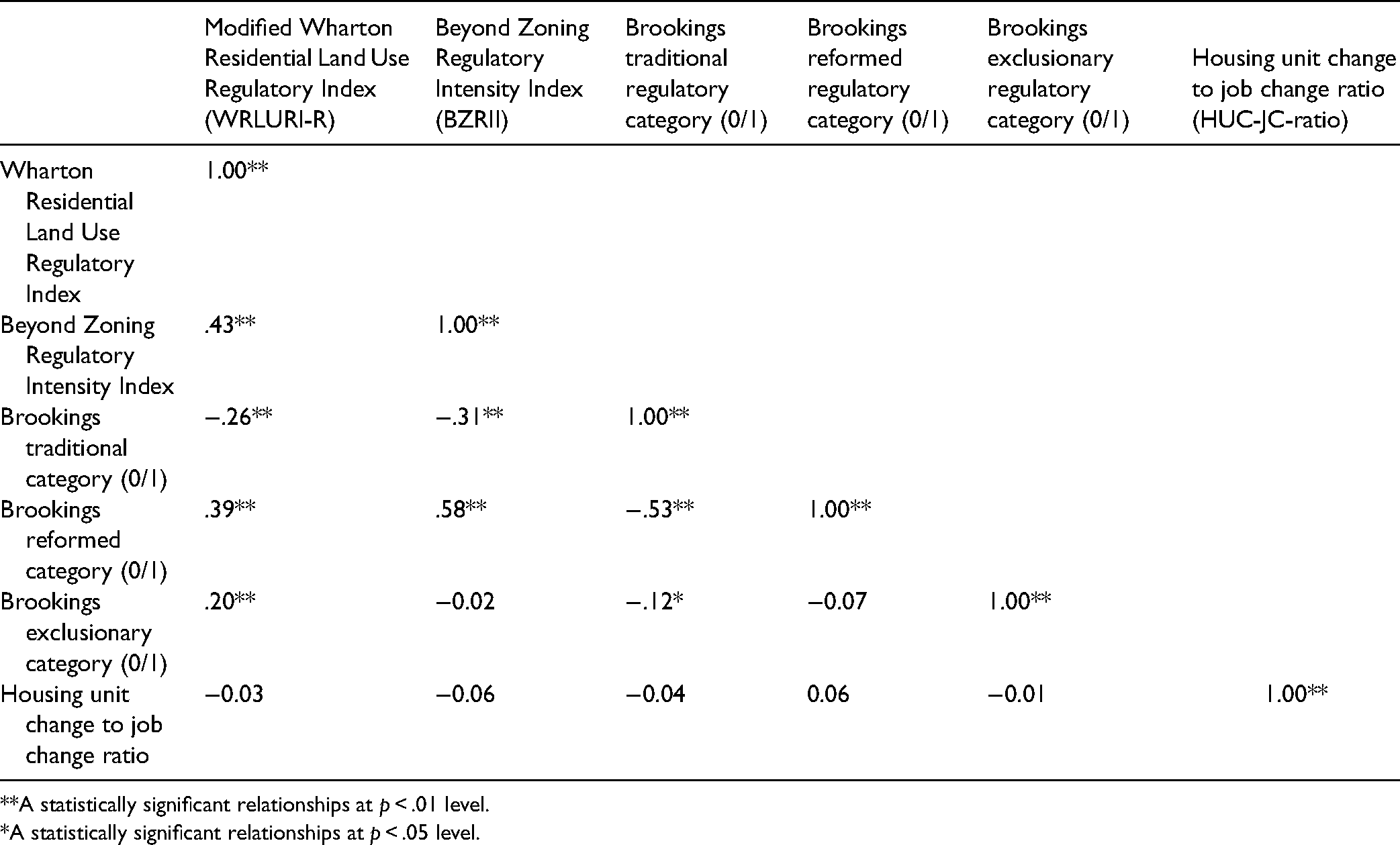
**A statistically significant relationships at p < .01 level.
*A statistically significant relationships at p < .05 level.
Except for the 0.58 correlation coefficient between the BZRII and the Brookings Reformed fixed effect variable, none of the correlation coefficients presented in Table 2 exceed 0.5. This indicates that they mostly measure different things and may be included together in the same regression model without worrying about potential overspecification. Particularly notable is the lack of any significant correlation between the HUC-JC-ratio variable and any of the regulatory index or categorical measures. If nothing else, this suggests that there is no immediate association between the administrative stringency of the local regulatory process and the degree to which that process limits new home construction levels when compared to job growth.
Measuring Home Values and Rents
Our outcome variables of interest are home values and rents. Each is measured differently. To measure rents, every year as part of the American Community Survey (ACS), the U.S. Census Bureau asks a sample of renters in every census tract to indicate their monthly gross rent. Gross rent is the combination of contract rent and monthly expenditures on heating and electricity.
The U.S. Census Bureau also asks homeowners about their monthly housing expenditures. But without knowing when a homeowner bought their home, their mortgage status and interest rate, or their local property tax rate, there is no way to relate monthly homeowner expenditures to current home prices. So instead of asking about home prices, the U.S. Census Bureau asks homeowners to estimate the current market value of their home.
How do homeowner-estimated current home values compare to current market prices? To find out, we compared the percentage change in median home values between 2010 and 2016 as reported in the ACS to the percentage change in the Case-Schiller Repeat Sales Price Index (now the S&P CoreLogic Case-Shiller Home Price Index) during the same period for the 20 metro areas where the two series overlap. On average, the Case-Schiller Index increased 12% faster during the 2010 to 2016 period than did ACS-reported median home values. The difference between the two measures is largest in Detroit ( + 25%), San Francisco-Oakland ( + 24%), and Seattle ( + 21%), and smallest in the greater New York City area ( − 3%), Denver ( + 3%), and Cleveland ( + 5%). The correlation coefficient between the two percentage change measures is a very high 0.92. The fact that the two measures mostly track together suggest that ACS-based median home value estimates are a reasonable substitute for market-based home prices, especially when reported for states and metropolitan areas with large ACS sample sizes.
Economic Vitality and Labor Market Measures
As noted previously, home values and rents are influenced by local economic growth. All else being equal, we should expect home values and rents to rise in places where jobs and wages are growing and to decline in places where they are falling. Because no single indicator can completely communicate the vitality of a local economy, we looked at several, including:
Labor force participation rates. Labor force participation rates measure the proportion of adults of working age currently working or looking for work. The more people who are working, the greater the amount of total income available for housing and other expenditures. With this in mind, we expect median home values and rents to be higher (and to have increased more) in metro areas with higher labor force participation rates. These data were obtained from the ACS. Average payroll per worker. Workers have more money to spend on housing in places where they are paid more (Mayock, 2016; Roback, 1982). We thus expect to observe a positive association between per-worker payroll levels
8
and median home prices and rents. These data were obtained from the U.S. Census Bureau's County Business Patterns series. Percent change in jobs, 2005–2016. New workers need places to live, so we would expect the demand for housing (and thus median values and rents) to be higher in metro areas with higher job growth rates. These data were obtained from the U.S. Census Bureau's County Business Patterns series. Real percentage change in payroll per worker, 2005–2016. As payrolls rise, workers will have more money to spend on all manner of goods and services, including housing. We should therefore expect to observe a positive correlation between recent payroll growth (measured per worker and after accounting for inflation) and median home values and rents. These data were obtained from the U.S. Census Bureau's County Business Patterns series.
In addition to jobs and wages directly affecting local home values and rents, we would also expect the home value and rent effects of local land use regulations to vary with the growth of the local economy. Simply put, supply constraints are less likely to have an observable effect where there is little growth to constrain. With this in mind, we constructed separate regression models for subsets of metropolitan areas based on their level of economic growth as measured in terms of job growth and per-worker payroll levels. In terms of job growth, we distinguished between three types of metropolitan economies: (1) “hot” economy metros in which the rate of job growth between 2005 and 2016 exceeded 10%; (2) “warm” economy metros whose 2005 through 2016 job growth rate was positive but less than or equal to 10%; and (3) “cold” economy metros that suffered job losses between 2005 and 2016. All else being equal, we would expect the adverse effects of local land use regulations and housing production shortfalls on median home values and rents to be larger in hot economy metros like Lafayette, Indiana (the metro area with one of the nation's highest job growth rate between 2005 and 2016), than in cold economy metros like Kokomo, Indiana (the metro area with the highest rate of job loss).
A second economic growth schema organizes metro areas into three groups based on their 2016 payroll (per worker) levels. The three groups include (1) high payroll economies in which per-worker payrolls in 2016 exceeded $43,820; (2) middle payroll economies in which 2016 per-worker payrolls were between $39,050 and $43,820; and (3) low payroll economies in which per-worker payrolls in 2016 were between $26,750 and $39,050. As with our job growth categories above, we would expect the adverse effects of local land use regulations and housing production shortfalls on median home values and rents to be larger in higher payroll economies like San Jose, California (the metro area with the highest 2016 payroll per worker) than in lower payroll economies like Brownsville, Texas (one of the lowest payroll per worker metro area).
Amenity Measures
There has been considerable research documenting the extent to which amenities like parks and open space (Geoghegan, 2002) and public services like school quality (Brasington, 1999) are capitalized into home values. For the most part, this capitalization effect occurs at the neighborhood or community level, but to the degree that an amenity or public service manifests itself regionally, it may also be capitalized into metropolitan-level home values and rents. Based on the available data, we created four sets of metro-scale amenity variables as controls. The first measures park land area per thousand housing units. 9 Research by Crompton (2005) and others Troy and Grove (2008) found the number and quality of nearby parks to be positively capitalized into home values.
Second, we included each metro area's average Walk Score 10 value. Walk Scores measure the geographic walking distance between every residential address and a standard set of nearby services and amenities. Measured on a 1-to-100 scale, Walk Scores provide a robust measure of the number and variety of neighborhood services, as well as the ease of getting to these services (Ewing & Clemente, 2013). Several recent studies have found Walk Scores to be positively, albeit unevenly, capitalized into housing and commercial real estate prices (Carswell et al., 2016; Pivo & Fisher, 2011).
Third, we included the share of adults in each metropolitan area as of 2016 that had obtained a bachelor's degree, as identified in the ACS. Research consistently is the connection between higher house prices and higher levels of educational attainment (Bischoff & Reardon, 2014; Eeckhout et al., 2010; Florida, 2010).
Finally, to control for climate and comfort (Glaeser et al., 2004), we obtained listings of heating and cooling degree days by state and census region from the U.S. Energy Information Agency. Heating degree days (HDD) are a measure of how cold a day is compared to temperature of 65°C. Cooling degree days (CDD) work the other way; they measure how hot a day is compared to a temperature of 65°C. Negative regression coefficients for both heating and cooling degree days would indicate a preference for a moderate climate. Descriptive statistics for these various regulatory, housing market, labor market, and amenity variables are included as (online) Appendix C.
Regression Results
This section interprets the results of multiple regression models comparing metropolitan-level measures of residential regulatory stringency to median home values and rents across multiple model specifications and robustness checks. As presented in Table 3, the first set of regressions explores the relationships between regulatory stringency and median home values. As presented in Table 4, the second set of regression models looks at the relationships between regulatory restrictiveness and median rents. The top half of each table considers home values (or rents) in 2016. The bottom half of each table looks at changes in home values and rents between 2005 and 2016.
Regression Results Comparing the Effects of Regulatory Stringency and Housing Construction Activity on 2016 Median Home Values and 2005–2016 Percent Change in Median Home Values.
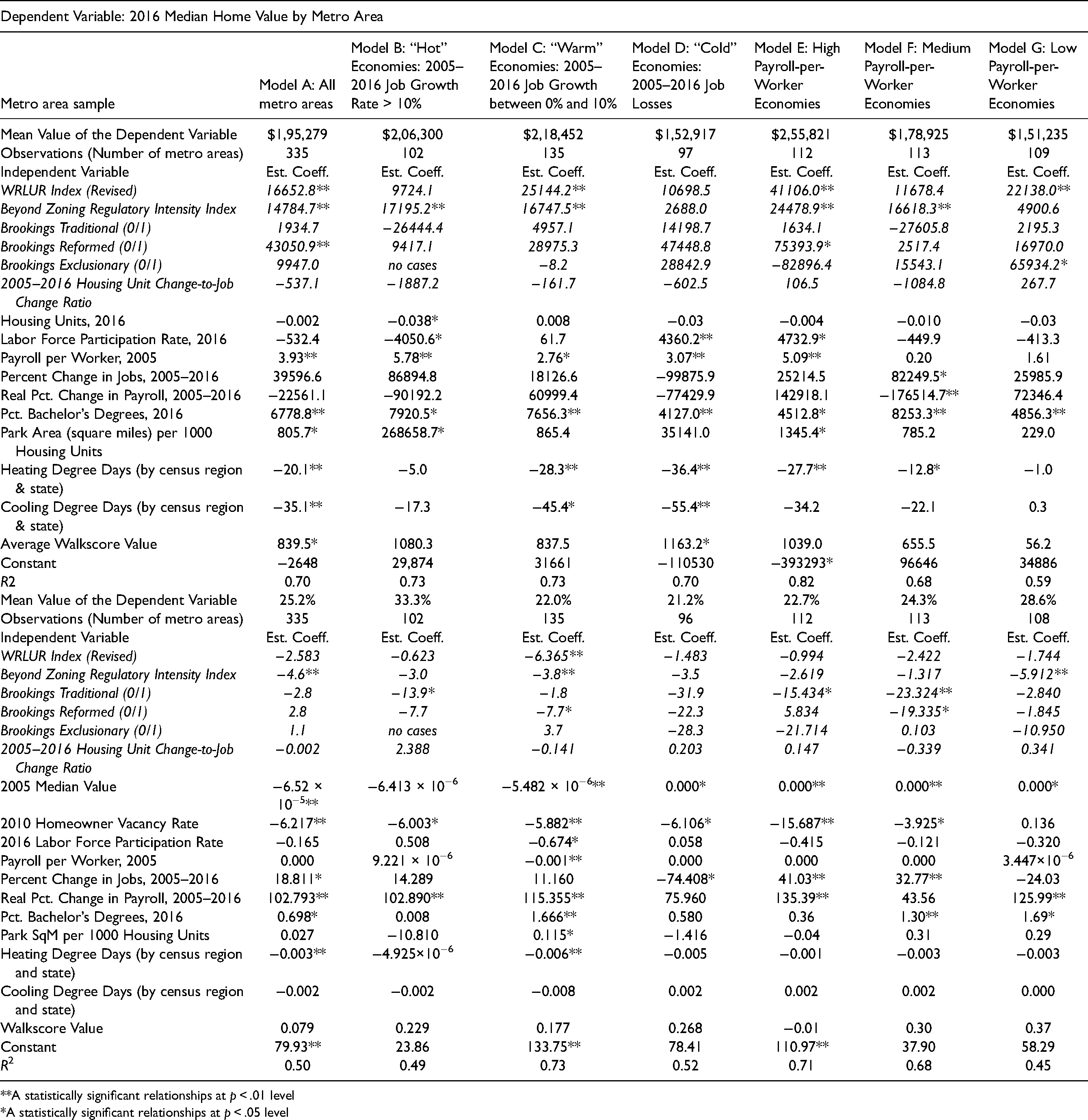
**A statistically significant relationships at p < .01 level
*A statistically significant relationships at p < .05 level
Regression Results Comparing the Effects of Regulatory Stringency and Housing Construction Activity on 2016 Median Rents and 2005–2016 Percent Change in Median Rents.

**A statistically significant relationships at p < .01 level.
*A statistically significant relationships at p < .05 level.
Each column of Tables 3 and 4 presents regression results for a different metropolitan area subsample. Model set A covers all 335 metro areas. Model set B covers 102 “hot” economy metro areas in which the 2005 to 2016 job growth rate exceeded 10%. Model set C covers 135 “warm” economy metro areas in which the 2005 to 2016 job growth rate was between 0% and 10%. Model set D covers 96 “cold” economy metro areas that lost jobs between 2005 and 2016. Model set E covers 112 payroll-per-worker metro areas in which average 2016 per-worker payroll levels exceeded $43,820. Model set F covers 113 metro areas with 2016 per-worker payrolls between $39,050 and $43,820. Last, Model set G covers 108 metro areas in which 2016 per-worker payroll levels fell below $39,050. By comparing the regression results across the different models, we can identify how the associations between regulatory stringency and housing values vary with metropolitan economic growth.
Given the great number and variety of metropolitan area housing markets, the different regression models explain median home values and rents surprisingly well. R2 values for the median home value regressions vary from 0.59 for the set of low payroll-per-worker metro areas, to 0.70 for all metro areas and to 0.82 for the medium payroll-per-worker metro areas. The median rent regressions are not as consistent but still strong: their R2 values range from 0.45 for the set of low payroll-per-worker metro areas to 0.5 for all metro areas, to 0.71 for this group. The rent and housing value change models explain between 42% and 73% of the growth in metro area median home values between 2005 and 2016, and between 26% and 54% of the growth in metro area median rents.
Looking past summary goodness-of-fit measures to coefficient estimates and significance levels, we can begin to answer the questions posed at the top of this paper:
Are restrictive land use regulations associated with more expensive homes everywhere? Based on our analysis of median home values in the 335 largest U.S. metro areas, the answer to this question is yes. All else being equal, a 1-point increase in WRLURI-R values—the equivalent of trading Boise, Idaho's regulatory system for Hartford, Connecticut's—is associated with a $16,652 increase in 2016 median home values. Similarly, a 1-point increase in the BZRII score is associated with home values rising another $14,785. Homes located in states with regulatory regimes categorized by the Brookings Institution as “reform”—meaning they supplement zoning restrictions with local growth-management ordinances—were $43,050 more expensive. Are the housing value effects of restrictive land use regulations larger in metro areas adding jobs at a faster rate and/or in areas with workers with higher pay? The answer to both of these questions is also yes, although the size of the regulatory premium varies depending on how metro-area job-growth rates and payroll levels are categorized. Among metro areas with “hot” and “warm” job economies, a 1-point increase in both the WRLURI-R and BZRII values is associated with a 2016 home value premium of between $17,000 and $42,000, compared to less stringently regulated metro areas. No such association existed for “cold” economies—those that lost jobs between 2005 and 2016. Among high payroll economies (e.g., those in which 2016 payrolls exceeded $43,820 per worker), a 1-point increase in the WRLURI-R and BZRII values is associated with a 2016 home value premium of more than $65,000, compared to less stringently regulated metro areas. In lower value-added economies, by contrast, the regulatory premium is between $17,000 and $22,000. Have home values increased faster since 2005 in metro areas with more restrictive land use regulations? In this case, the answer is no. Regardless of which metro area subset was modeled, there was no association between higher WRLURI-R values and higher rates of home value growth between 2005 and 2016. In the case of BZRII scores, higher values were associated with slightly lower rates of home value growth. The clearest interpretation of this result is that home values in stringently regulated markets were higher initially, thereby moderating their potential for later growth. Are more intrusive land use regulations also associated with systematically higher apartment rents? Here again, the answer is yes. All else being equal, a 1-point increase in the WRLURI-R value was associated with a $45 per month (or 7%) increase in 2016 rents. Similarly, a 1-point increase in the BZRII score was associated with an $11 per month (2%) rent increase. Apartments in states with regulatory regimes categorized by the Brookings Institution as “reform” rented for $74 more per month and those in states with “exclusionary” regulatory regimes rented for an additional $122 per month. The WRLURI-R rent premiums were highest among “warm” job growth and high payroll per worker metro areas. Did median rents in stringently regulated housing markets increase faster between 2005 and 2016? As with home values, the answer to this question is no. The relationships between housing supply flows and home values are complicated. Regardless of which sample was analyzed, there was no statistically significant association between 2016 home values or home-value gains and the housing-unit-change job-change ratio (HUC-JC-ratio). Simply put, home values in metro areas where housing construction failed to keep pace with job growth were not consistently higher than in metro areas where housing construction led job growth. There are two possible explanations for this counterintuitive finding. The first is that the HUC-JC-ratio does not reliably measure housing supply flows. The second explanation is that the relationships between home values and housing production shortfalls (compared to job growth) are not consistent across metropolitan areas. When measured at the metropolitan scale, home values increase with local economic growth. The extent of this effect depends on how economic growth is measured. As expected, higher payroll-per-worker levels are associated with higher home values. They are not, however, associated with faster home-value growth. By contrast, single-year home values are not associated with faster job and payroll growth, but home-value growth rates are. This is true regardless of the metro area sample considered. Simply put, faster economic growth encourages home values to increase more quickly regardless of metro area, but it does little to explain underlying home value differences between metro areas. Median rents in 2016 were mostly higher in metro areas with higher per-worker payroll levels. These rent-premium relationships mostly parallel the home-value premium relationships identified above, although they are generally smaller when expressed in percentage terms. As with home values, higher housing supply flows did not affect either rents or changes in rents. Again, this finding is counterintuitive but could be the case because of challenges around measurement or variation across metropolitan areas in our sample.
Beyond issues of land use regulation, the regression results presented in Tables 3 and 4 provide further insights into the factors shaping home values and rents when measured at the metropolitan scale:
These findings are subject to a variety of caveats, starting with how the WRLURI-R and BZRII indices are constructed. Although an improvement over the usual method of using simple dummy variables to indicate the presence or absence of regulatory programs, neither the WRLURI-R nor BZRII measure fully captures how the regulatory process is experienced at the project level or the high level of regulatory variation within metropolitan areas. The same is true for the two dependent variables: median home value and median rent. Both vary widely within every metropolitan area. Median value is also self-reported instead of being based on current market prices, and is drawn from a sample of all homeowners, not just recent buyers or sellers. The housing supply flow measure, HUC-JC-ratio, has its own issues. It is a cumulative measure of relative housing supply shortfalls, rather than a period-specific measure of how much market inventory is available. This last shortcoming is likely the reason behind its poor showing in the regression models. Although necessary because of a lack of detailed local data, our method of using state-level WRLURI-R and BZRII scores to estimate metropolitan-level values is also open to debate. Altogether, these caveats call into question the precision of some of our coefficient estimates as well as their applicability at the intrametropolitan scale.
A Closer Look at Local Land Use Regulations and Housing Affordability
Would liberalizing restrictive land use regulations improve housing affordability? And if so, by how much? To find out, we used the regression results presented in Tables 3 and 4 to re-estimate median home values and rents, assuming that current WRLURI-R and BZRII values would be reset to 0 and 2.8, respectively. (A WRLURI-R value of 0 means a metro area is neither overregulated or underregulated, and 2.8 is the average BZRII score across all 50 states.) We will henceforth refer to this situation as relative regulatory neutrality, or RRN.
For highly regulated metro areas like Honolulu or San Francisco-Oakland, RRN would entail rolling back regulations and process requirements. Such changes would increase the ability of residential developers to undertake projects “as-of-right” according to local zoning and not have to go through additional reviews. In less regulated markets like Laredo or Charleston, moving to RNN would require expanding the level of regulatory stringency. Because we do not regard such an outcome as likely, we left the WRLURI-R and BZRII scores of underregulated markets as is.
Having updated each metro area's WRLURI-R values and BZRII scores to make them consistent with the RRN scenario, we then used the regression results presented in Tables 3 and 4 to compare RRN-based median home values and rents to their actual 2016 values, as reported in the ACS. The results of these RRN versus ACS simulations are presented in Figure 1 for the 15 least affordable homeownership and rental housing markets in each job market temperature category. The data labels attached to the lower bars indicate the percentage difference in estimated monthly rent or mortgage payment between the RRN scenario and current regulatory levels.
To make it easier to compare changes in homeownership affordability, we converted estimated home values to monthly mortgage payments by assuming that all homebuyers would finance their homes with a 30-year fixed-rate mortgage with a 3.5% annual interest rate based on a loan-to-value ratio of 80%. Because the metros areas listed in each panel of Figure 1 are the least affordable in each job market temperature category (based on the share of households with excess cost burdens), these comparisons represent a sort of best-case scenario of how liberalizing local land use regulations could contribute to making housing more affordable.
As expected, the results vary by job market category as well as by metropolitan area. Among the 15 least affordable “hot” job market metro areas (i.e., those with 2005–2016 employment growth rates above 10%), achieving RRN would result in a decline in monthly mortgage payments ranging from as much as 29% in Bakersfield to virtually nothing in Charleston, Laredo, and Greeley. Metro areas in characteristically overregulated states like California and Florida would generally see bigger declines, while those in underregulated states like Texas and South Carolina would not be affected. On average, monthly mortgage payments would fall by 12%, a significant amount, especially in very high-cost markets like Seattle and San Jose.
Among the 15 least affordable “warm” job market metro areas, moving toward an RRN situation would result in monthly mortgage payments declining by as much as much as 30% in California inland markets like Visalia, Modesto, and Riverside-San Bernardino. In absolute terms, the decline would be even larger among California's expensive coastal markets like San Francisco and Los Angeles, averaging more than $300 per month.
Among the 15 least affordable “cold” job market metro areas (i.e., those that lost jobs between 2005 and 2016), moving toward an RRN situation would have little effect on monthly mortgage payments. This is not because they are overregulated, but rather because we observed no empirical association between regulatory obtrusiveness and home values.
The rent reductions resulting from liberalizing local land use regulations are quite a bit smaller, averaging just 3% among the “hot” job market metro areas and 10% among “warm” job market metro areas. This is because apartment rents are more sensitive to the current balance between rental supply and demand as manifested through vacancy rates, while home values are more reflective of buyers’ and sellers’ future price expectations.
These are all model-based static estimates. In practice, housing values and rents are both path-dependent, meaning that they do not move downward the same way they move upward. To the extent that liberalizing local land use regulations would affect future market outcomes, it would probably occur as a slowdown in future price increases—as additional suppliers work themselves onto the market—rather than as immediate property value or rent declines. Regardless, each market would respond differently. In markets like New York City and San Francisco, where demand sometimes seems inexhaustible and a limited supply of buildable sites means that new construction often takes the form of redevelopment, it might take many years for the benefits of deregulation to make themselves known. In other markets where single-family-only zoning and other restrictions are creating artificial land shortages and preventing multifamily homebuilders from bringing projects to market, the effects of deregulation would be quickly apparent, especially on the rental apartment side.
Conclusions and Policy Recommendations
Three things set this work apart from prior studies. The first is its comprehensive geographical coverage: it explores the relationships between local land use regulations and recent housing market outcomes in more than 85% of U.S. metropolitan areas, not just the largest, the most expensive, or the fastest growing. Second, it makes use of multiple representations of local regulatory stringency, including an input representation as captured by an updated version of the Wharton Residential Land Use Regulatory Index (the WRLURI-R measure); a second input measure that captures the full range of government interventions in the private land market, the BZRII; a categorization scheme produced by Brookings Institution researchers organized around the relationships between zoning and planning; and a housing supply outcome measure that compares housing construction activity with job growth. Third, it allows the relationships between local land use regulations and local housing-market outcomes (as represented by median home values and median rents) to vary according to local economic growth. This combination of improved spatial coverage, multiple regulatory measures, and increased attention to the demand side of the story allows us to develop a more nuanced understanding of how and where restrictive land use regulations have their most pernicious effects. Among its most important findings:
When measured at the metropolitan scale, more stringent land use regulations are indeed associated with higher housing values and rents. This association extends well beyond a few high profile coastal metropolitan areas. As expected, the association between stringent land use regulations and higher home values and rents is stronger in higher payroll-per-worker economies and those experiencing significant job growths. Local land use regulations have little association with home values and rents in low payroll-per-worker and job-losing economies. When measured at the metropolitan scale, the associations between housing construction activity and home values and rent levels vary so idiosyncratically that one cannot say that there is a consistent relationship between the flow of new homes and local housing price levels. This isn’t to say that there is no relationship between housing supply constraints and housing prices—there clearly is—but rather, that the specifics of that relationship vary locally. Median home values and rents rose no more quickly during 2005 to 2016 in highly regulated metropolitan areas than in less regulated ones. Instead, the growth in home values and rents during this period was much more strongly associated with local employment and payroll growth. Relaxing restrictive land use regulation has some potential to make housing more affordable, especially in high-priced metropolitan areas in California and Florida. Depending on how builders respond, these affordability improvements are more likely to take the form of slower rates of future housing-price growth than immediate price reductions.
These findings have important practical implications for the state and local officials who create and administer local land use regulations. The first is that they should focus more on providing significant and permanent regulatory relief than on maximizing near-term home construction. Making it easier for a few developers to build a few high-density projects in a few locations is unlikely to have as sizeable an effect on home prices and rents as reforming the local regulatory process to make that process more transparent and less ad hoc. Doing so will also help promote increased builder competition, which is a principal source of reduced housing prices.
Second, the best way to provide constructive regulatory relief is not to weaken or liberalize community-wide regulations, but instead to make it easier for local builders to respond to place-specific market demand. This is most easily done by establishing “as-of-right” development zones in high-demand areas so that builders whose projects meet current zoning and subdivision requirements need not go through an extended and discretionary approval process. As-of right development zones need not cover all or most of a community, but they do need to be present in sufficient numbers and in enough places to enable builders to develop at scale. Because it necessarily takes a long time for increased construction activity to translate into more affordable prices and rents, the designation of as-of-right housing construction districts should be accompanied by some form of inclusionary housing requirement that allocates a portion of the additionally permitted units for low- and moderate-income households.
Finally, it is important to realize that regulatory relief in and of itself will not be sufficient to meet the affordable housing needs of low- and moderate-income renters in any U.S. metro area. Regulatory relief will certainly make it easier for developers to build additional market-rate apartments. Even so, the gap between market rents and affordable rents is currently so large that relying on additional housing construction to gradually filter down to moderate- and low-income households alone has no merit. The only effective way to deliver affordable housing to low-income households is to subsidize it in some form. One local mechanism for doing just that is inclusionary zoning, which requires builders to set aside a specific share of market-rate units for low- and moderate-income households. Even when inclusionary housing works as intended, additional subsidies may be needed to reach very low-income families.
Beyond reducing local development regulations in a manner that promotes appropriate housing construction, how might the local regulatory process be streamlined? As a starting point, state governments should require local municipalities to document the beneficial outcomes (including avoidance-of-harm outcomes) associated with particular environmental, growth management, and single-family zoning programs, with an eye toward eliminating or modifying those unable to demonstrate they create a measurable local or cumulative benefit. Similar regulation-pruning initiatives have been undertaken by HUD and the Office of Management and Budget in the past, but they have foundered on the fact that local land use regulations are creatures of state and not federal law. Many states already apply this type of “nexus” prerequisite to development impact fees, and it should be possible to extend it to other types of local land use regulations as well.
Footnotes
Declaration of Conflicting Interests
The authors declared no potential conflicts of interest with respect to the research, authorship, and/or publication of this article.
Funding
The authors received no financial support for the research, authorship and/or publication of this article.