“GANZ RASCH”

Abstract

This article presents a new and freely available tool for performing analyses according to the Rasch model (RM) and the latent class analysis (LCA). The software allows for the estimation of the model parameters and offers several measures of model fit. A graphical user interface (GUI) provides access to numerous options regarding data, models, and output. For educational purposes, an optional annotate feature allows to augment the output with brief explanations and citations regarding the procedures. Based on published data, the features of GANZ RASCH are briefly illustrated in two worked examples. The program intends to combine ease of use while allowing for performing a full-fledged analysis, thus targeting a wide range of users.

Keywords

Rasch model latent class analysis parameter estimation assessment of model fit

Introduction

The Rasch model (RM; Rasch, 1960, 1966) is a probability model for a dichotomous random variable X_vi involving the two real-valued latent parameters θ_v (v = 1 … n) and β_i (i = 1 … k). It is a member of the exponential family and the probability of a keyed (positive) response (usually coded with one) is

p (X_{v i} = 1 | θ_{v}, β_{i}) = \frac{e^{θ_{v} - β_{i}}}{1 + e^{θ_{v} - β_{i}}} .

(1)

The major application of the RM is psychometrics, where θ_v represents the proficiency of respondent v to solve item i (e.g., in an achievement test) and β_i describes the difficulty of item i. The column and the row marginals are minimal sufficient statistics for the item and the person parameters, respectively. One of the most prominent model features is specific objectivity, stating, in short, that the parameters β_i can be estimated independently of the level and the distribution of the parameters θ_v in the sample, and vice versa (cf. Rasch, 1966, p. 104). Therefore, it allows for both the estimation of the item parameters even if the sample is not representative and, analogously, for the quantification of a respondent’s proficiency independently of the actual items used, given they are in line with the model. The latter forms the basis for adaptive testing (cf. van der Linden & Glas, 2010) and Item Banking (cf. Timminga & Adema, 1995). Note that using an individual’s unweighted score for describing his or her performance tacitly assumes the RM to hold.

Numerous parameter estimation methods have been developed, differing with respect to their assumptions: One can apply the unconditional (or Joint) maximum likelihood method (UML or JML; cf. Baker & Kim, 2004; Molenaar, 1995), where item and person parameters are alternately updated. Unfortunately, this method suffers from the so-called incidental parameter problem (Neyman & Scott, 1948). In short and applied to the present case, it means that the item parameters β_i (which are structural parameters) cannot be estimated consistently in the presence of the person parameters θ_v (which are incidental or nuisance parameters). One way to circumvent this problem is to apply marginal maximum likelihood estimation (MML, cf. Baker & Kim, 2004; Molenaar, 1995), in which a proper distribution of the incidental parameters has to be assumed and only the hyperparameters of this distribution (which are now likewise structural parameters) are estimated. However, this approach will not be further pursued in the present context.

One estimation method, fully taking advantage of the existence of sufficient statistics, is the conditional maximum likelihood estimation method (CML), originally proposed by Rasch (1960) and further elaborated by Andersen (1970). To put it in a nutshell, the item difficulty parameters are estimated by conditioning on the sufficient statistics of the person parameters. This fact entirely liberates us from making any distributional assumptions, yet delivers unbiased and consistent item parameter estimates. The person parameters are estimated separately by means of a maximum likelihood estimation, using the item parameter estimates obtained before. It is intrinsic to this approach that estimates for respondents with perfect or zero scores approach plus or minus infinity. Nevertheless, estimates for such cases can be obtained by means of a modified procedure of Warm (1989), which attenuates the unbound growth of the estimates.

The three methods considered so far are iterative by nature. In contrast, a closed form estimation method is at our disposal as well, namely, the pairwise method (cf. Fischer, 1974, p. 268; Molenaar, 1995, p. 49). It excellently suits didactical purposes, as it can be accomplished with a pocket calculator. However, this procedure is limited by requirements likely to fail in small data sets or when item difficulties vary largely (see below).

Numerous methods for assessing the model fit have been proposed, a conclusive overview of which can be found in Glas and Verhelst (1995). One method, which is directly derived from specific objectivity, is the conditional likelihood ratio test (LRT) according to Andersen (1973). This test assesses the subgroup invariance of item parameter estimates (which is a consequence of specific objectivity) by means of splitting the sample into g subgroups (horizontal split). Originally, Andersen proposed splitting along the proficiency scale θ, that is, according to the score, but any other criterion of substantive interest can be taken as well. In the case of a two group split (e.g., using the score median as split criterion), the subgroup item parameter scatterplot can be used for a rough appraisal of model adequacy: Points scattering closely around the 45° line substantiate model fit. In a similar manner, the Martin-Löf-Test (MLT, cf. Glas & Verhelst, 1995) assesses the unidimensionality assumption by splitting the item set into two groups (vertical split).

Another model of equal importance for social sciences is the latent class analysis (LCA; Dayton, 1998; Formann, 1984; Lazarsfeld, 1950). In contrast to the RM, the LCA assumes the latent variable to be categorical, which complies with the assumption of mutually exclusive and exhaustive subpopulations (the “latent classes”). Each of the latent classes exhibits a constant probability for its members to respond positively to a manifest dichotomous item. The LCA allows for the estimation of both the conditional item probabilities (given the latent class) and the class sizes. It belongs to the mixture models, as the latent classes appear “mixed” in the data, which resulted in using the term “unobserved heterogeneity” as well. This approach might be preferable if a latent classification (or typology) is assumed or is to be achieved. For dichotomous items, the model equation is

p (X_{c i} = 1 | π_{c}, π_{i c}) = \sum_{c = 1}^{m} π_{c} \prod_{_{i = 1}}^{k} π_{i c} .

(2)

The parameter

π_{c} (c = 1... m, Σ^{m}_{c = 1} π_{c} = 1)

represents the sizes of the latent class c and

π_{i c}

(sometimes written as

π_{i | c}

π^{(c)}_{i}

) denotes the conditional probability that item i is solved (or endorsed) by members of the latent class c (cf. Dayton & Macready, 2007). Note that the number of latent classes, m, is not a model parameter, rather it has to be ascertained prior to estimation based on theoretical considerations. The probabilities

π_{i c}

allow for the identification of marker items of a latent class: A marker item has a distinctive probability in one class and therefore allows for the characterization of this class in terms of substantive theory.

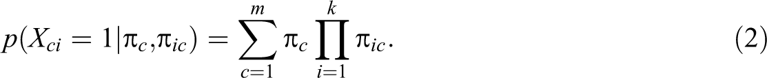
Based on the response pattern frequencies, maximum likelihood estimates of the model parameters $π_{c}$ and $π_{i c}$ are obtained by means of an expectation-maximization (EM)-algorithm (Dempster, Laird, & Rubin, 1977; McLachlan & Krishnan, 1997). Note that the likelihood function of the latent class model can be multimodal, therefore the parameter estimation should be repeated with several sets of starting values. This repetitive procedure increases the chances of identifying the parameter estimates associated with the global rather than a local maximum of the likelihood function. Based on these item parameter estimates, each respondent’s manifest class membership probability can be determined ex post by applying Bayes’s theorem (cf. Dayton, 1998, p. 8). A modal decision then allows for assigning each respondent to the class he or she most probably belongs to. Of course, such a decision can be clear-cut or highly ambiguous, which is reflected by the entropy measure, averaging the allocation probabilities of subjects per class (cf. Ramaswamy, Desarbo, Reibstein, & Robinson, 1993).

The overall goodness of fit can be assessed by means of the family of power divergence statistics (Read & Cressie, 1988), which covers several procedures to compare the observed and the expected response pattern frequencies. Probably the most prominent member of this family is the Pearson test statistic (cf. Dayton, 1998; Formann, 2003); however, Read and Cressie (1988) argue that a certain modification of this method is preferable for theoretical reasons (p. 96). The Freeman–Tukey test (Freeman & Tukey, 1950) and the Wilks’s likelihood ratio statistic (Wilks, 1938) are also members of the power divergence family of statistics. Formann (2003) provides an excellent overview of these methods.

Several other goodness-of-fit measures have been proposed as well. In this context, the information-based indices (Akaike’s Information Criterion [AIC], Akaike, 1973; Sakamoto, Ishiguro, & Kitagawa, 1986; Bayesian information criterion [BIC], Schwarz, 1978; consistent AIC [CAIC], Bozdogan, 1987; AIC, Hurvich & Tsai, 1989) play a crucial role. These indices allow for comparing different latent class analyses for the same data, covering a varying number of latent classes. Basically (at the risk of oversimplification), these indices rely on the sum of minus two times the log likelihood of the final estimation step and the (weighted) number of parameters used in the model. This results in a small index if the model describes the data well while pursuing the desideratum of parsimony. Therefore, the model with the lowest index among several candidate models is chosen. A very indicative introduction to information indices is provided by Anderson and Burnham (2002).

GANZ RASCH¹: A New Program

This article presents a new software, allowing for the estimation of the parameters of the RM and the LCA and for the assessment of fit of either model. It employs a graphical user interface (GUI) with tabs resembling the workflow of a typical analysis: The three main steps of an analysis (load data, choose model, and view output) form the top level tabs containing subsections (Level-2 tabs) for purposes associated with the respective step. A permanently visible Quick Navigation bar on the left-hand side of the program window allows for directly accessing all Level-1 and Level-2 tabs with one mouse click.

The program has been developed under the MS-Windows^® operating system and was successfully tested under both the Linux and the Mac operating systems, using an emulator.²GANZ RASCH reads American Standard Coding for Information Interchange (ASCII) data in free format, Statistical Package for the Social Sciences (SPSS) system data files (*.sav), and supports direct data entry. It allows for integer weighting of records and for data export to both ASCII and SPSS. Currently, the program is designed for the analysis of dichotomous items and expects responses to be coded with zero or one. Missing values have to be flagged (e.g., with codes –1 or 99).

All models default to essential options covering parameter estimation and model fit, hence standard analyses can be performed with just a few mouse clicks. The RUN button is always visible, yet disabled if required input is missing. For users less acquainted with the models, the program output might appear enigmatic. In trying to provide some relief, an ANNOTATE OUTPUT option allows for augmenting the listing with notes concerning the methods applied and hints for further reading. Of course, such a feature can never substitute a thorough study of the relevant literature—but it might provide easier access to the topic and direct users toward useful resources. Furthermore, some plots allow for a quick visualization of crucial results.

Models and Algorithms

In essence, GANZ RASCH covers the two models introduced above. Additionally, some basic calculations according to the so-called classical (true-score) approach are provided. For the RM, the CML estimation is the default method; nevertheless, several others are available as well. These are the JML and the pairwise method, which have been mentioned above. The latter may support classroom applications, allowing students to check their results obtained by hand. Additionally, the program provides the so-called MINCHI method (Fischer, 1974, p. 269; Molenaar, 1995, p. 50) and the PROX method (Wright & Stone, 1979). Concerning the person parameters, both the maximum likelihood and the modified estimates according to Warm (1989) are displayed.

The Andersen and the Martin-Löf tests allow for an inferential check of assumptions specific to the RM, providing several options allowing for a very flexible use of these tests. The graphical model check described above is provided as well. In order to detect conspicuous items, GANZ RASCH provides graphs of the empirical and the model-based item characteristic functions. A special option superimposes the latter two, which may serve as a guideline for detecting possible model deviations by observing discrepancy between the two curves. This check is supplemented by the χ² test of Bock and Lieberman (1970; cf. Embretson & Reise, 2000, p. 235), which compares observed and expected frequencies associated with the two curves. The residual based χ² statistic along with the INFIT and the OUTFIT mean square statistic (cf. Wright & Masters, 1982, p. 100) also allow for the evaluation of the fit of the RM on an item-by-item basis. Plots of the item information function and test information function (IIF and TIF, cf. Embretson & Reise, 2000, pp. 183–185) tell us, in which domain of the latent trait θ a given set of items allows for a most precise measurement. The different IIFs can be plotted one by one, all in one, and they can be superimposed with the TIF.

The LCA is supported for up to 12 latent classes and employs the EM algorithm. Again, several methods of assessing model fit are provided, including, for example, four information-based criteria and four power divergence statistics. Two plots seem noteworthy: First, a line diagram of the item probabilities per class (the $π_{i c}$ ) allows for recognizing marker items at a glance. Second, a histogram of the class allocation probabilities supports a quick assessment, whether the allocation of individuals to classes was rather clear-cut or ambiguous.

Although the main focus of the program is on probabilistic models, some basic classical psychometric indices—like the item-total correlation (uncorrected and corrected) and the lower bound of reliability according to Cronbach (coefficient alpha; Cronbach, 1951)—are displayed as well. The covariance and the correlation matrices can be requested, an option that might prove useful for further use, for example, with a structural equation modeling software.

Selected Features Specific to GANZ RASCH

This section highlights some technical features possibly distinguishing GANZ RASCH from other software. Some acquaintance with the various models facilitates the users’ comprehension of these distinctions.

RM: Parameter estimation with the CML method

Wright and Douglas (1977) appreciate the “theoretically ideal” (p. 573) CML method, but they consider it computationally too costly for practical application, because a complex combinatorial task has to be performed (involving the elementary symmetric function, γ_r, cf. Baker & Harwell, 1996; Fischer, 1974). However, this function can now be evaluated in a split second (cf. Molenaar, 1995, p. 46). GANZ RASCH provides the most precise summation method (Gustafsson, 1980; default), the possibly faster but slightly less precise difference method (Fischer & Formann, 1972), and a truly recursive method.

RM: Parameter estimation with the pairwise method

The pairwise method is of interest, for it delivers virtually the same estimates as the CML method while it is at the same time computationally extremely simple and fast. However, this method has one limitation, possibly narrowing down its applicability: For each pair of items, both response patterns 0–1 and 1–0 have to be observed at least once. This is not much of a problem when samples are large and items are of similar difficulty. However, the combination of easy and difficult items is likely to violate this requirement, unless the sample is sizable. However, the program optionally provides a corrective procedure, which is experimental, yet promising: Unobserved combinations are given a frequency of one. While this correction (demonstrably) does not affect other item’s estimates, it retains the method applicable. Note that this correction is similar to the Bayesian approach of assigning priors to the likelihood function (which would in this case be the Dirichlet distribution). But while in a Bayesian framework, one would add a value of one to each pattern frequency (i.e., without scanning the data), GANZ RASCH only fills in the missing ones, “after having had a look at the data.”³

RM: Goodness of fit with the Andersen test

The program supports several split methods with great flexibility: (a) When deciding for the score median split, one can choose with a mouse click whether to put respondents realizing exactly the median value into the lower or into the upper score group. (b) If the median was either beyond a value of two or above k−2, one group would vanish and the procedure would fail. In that case, an (optional) adaption allows for automatically increasing or decreasing the cutoff value, until both groups contain observations. This feature is useful for heavily skewed score distributions. (c) GANZ RASCH supports the proposal of Formann (1981; see also Molenaar, 1983) to split along an item of the scale to be analyzed, which is interesting from a substantive point of view. (d) GANZ RASCH offers the split using the a posteriori group membership allocations of a two group LCA, according to a proposal of Formann (1983). (e) GANZ RASCH allows for an arbitrary number of random splits to be applied.

RM: Goodness of fit with the Martin-Löf test

The MLT (which is equivalent to the later independently developed R _1c-statistic, Glas, 1988; Glas & Verhelst, 1995) allows for the detection of violations of the unidimensionality assumption by comparing two sets of items by means of a LRT. Usually, such a split is performed with regard to the items’ content, hence they have to be selected manually. As a novelty, GANZ RASCH offers an additional AUTOSPLIT option: after estimating the item parameters for the total data set, items will be split automatically according to their difficulty estimates (mimicking the score median split from the Andersen test).

RM: Alpha inflation when applying multiple goodness-of-fit tests

Each test introduces a risk α of committing a Type I error of falsely rejecting the null hypothesis of model fit. When m > 1 tests are applied, the overall (familywise) risk of falsely deciding at least once increases considerably. For that reason, a modified value $α^{*} = 1 - m \sqrt{1 - α}$ can be applied to each test in order to warrant the familywise risk α_FW not to exceed a desired level (cf. Hays, 1994, sec. 11.13). GANZ RASCH supports this approach by counting the number of tests performed and automatically delivering the respective α* for a familywise risk α_FW of 1%, 5%, and 10%.

Worked Examples

A historical example will be used for demonstrating the usage of GANZ RASCH, namely, the data on role conflict according to Stouffer and Toby (1951). The intention of this study was to shed light on the question, whether social obligations form a unidimensional trait reflecting the continuum of particularistic versus universalistic, according to Parsons (1949). Four stories were presented, involving a car accident (giving false witness in favor of a friend), drama critic (go easy on a friend’s bad play), insurance doctor (shade doubts on a friend’s diagnose), and a board of directors meeting (insider trading). Originally, the scalogram analysis according to Guttman (1950) and the latent distance model according to Lazarsfeld (1950) were applied, obtaining a rather good model fit in both cases. Andersen (1980) and Formann (1995) have reanalyzed a subsample of 216 respondents with the RM. This analysis will be repeated here to demonstrate the program briefly. Furthermore, the same data set is used to apply LCA in the same way as by Formann (1995).

Example 1: The RM

After reading the data from SPSS, the default options (CML estimation, Andersen test applying the median split, and the graphical model check) were retained and three additional random splits were selected. The part of the program output containing the parameter estimates is depicted in Figure 1 . The item parameter estimates are perfectly in line with those reported by Andersen (1980, p. 290), and the person parameter estimates perfectly fit those presented by Formann (1995, p. 247).

Figure 1.

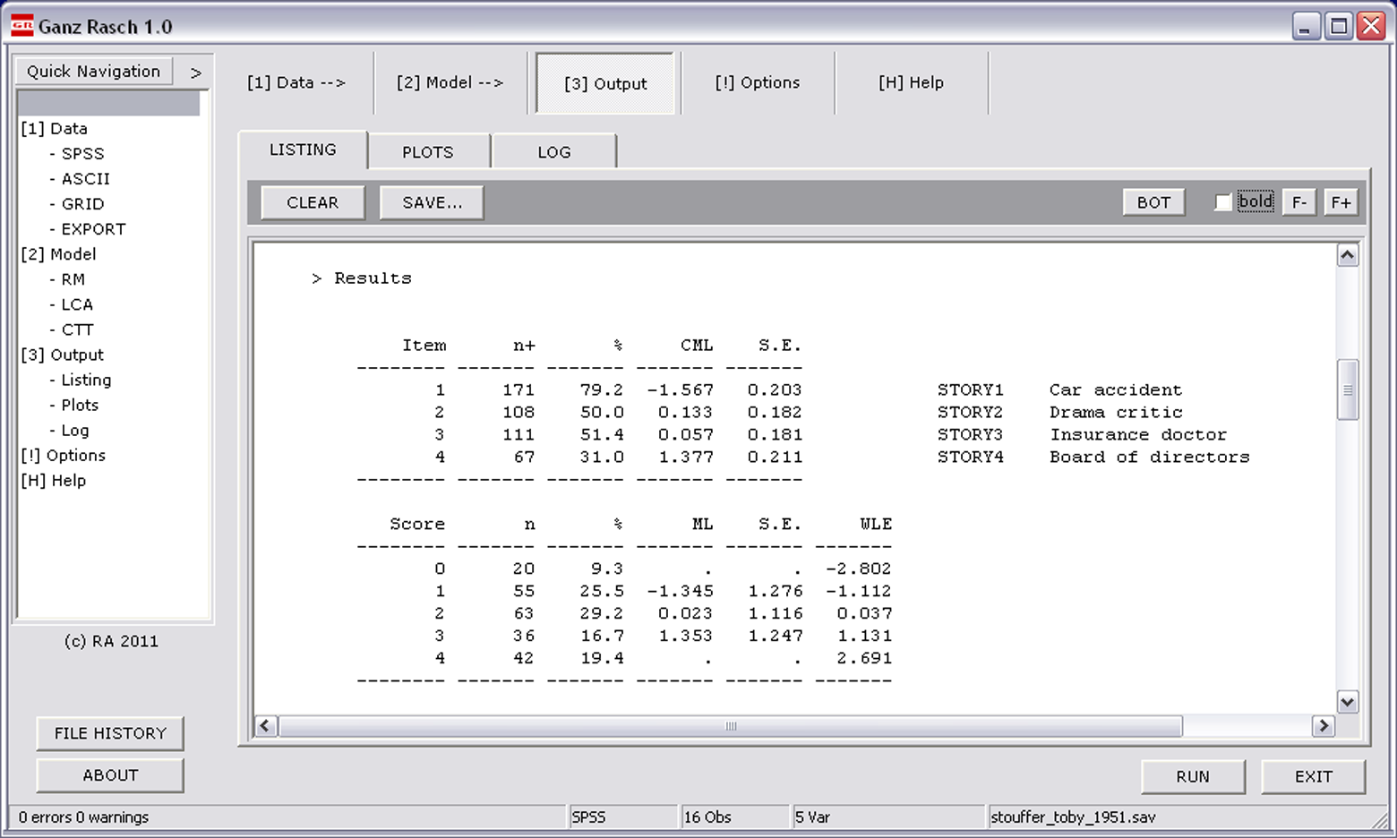
Parameter estimates of the Rasch analysis of the Stouffer and Toby (1959) data.

The LR test statistic was .118 with three degrees of freedom, yielding a p value of .990, therefore the null hypothesis of model fit is not rejected according to this analysis. The same holds true for the three random splits, showing similar results, $χ^{2}_{[3]}$ = 4.107, p = .25; $χ^{2}_{[3]}$ = 2.136, p = .545; $χ^{2}_{[3]}$ = 1.493, p = .684. Altogether, four tests have been performed, therefore GANZ RASCH outputs the corrected $α^{*}_{[5 % F W]}$ = .012741 as well. According to the corrected value, again none of the three tests would lead to a rejection of the null hypothesis of model fit. This is in agreement with the findings of Formann (1995) “[…] that the Stouffer and Toby data conform to the RM to a very high degree.” (p. 249). Of course, the failure to reject the model cannot be taken as evidence of model fit. However, the more often a model passes efforts to reject it, the greater becomes its corroboration (in the sense of Popper).

Example 2: The Latent Class Model

The application of the Latent Class Model shall be demonstrated with the same data set, applying a two- and a three-class solution. In contrast to the first example, data shall be read from ASCII: The file contains five columns representing the four variables (coded with zero and one) followed by one column containing the frequency of the respective pattern. In the top line, the variable names are provided. After opening the file through DATA > ASCII > OPEN, its content is listed in a preview panel. A click on the READ button loads the data, which are then displayed in the [1] DATA > GRID tab. There, the four analysis variables have to be selected and the weight variable can be chosen from the Weight cases by… pull down combo box.

Next, the desired model details have to be chosen from the [2] MODEL > LCA tab. Essentially, only the number of classes to be estimated have to be set. After clicking on RUN, the output appears. The parameter estimates perfectly match those reported by Formann (1995, p. 249). The two classes show a clear distinction, as the first class beats the second in having higher probabilities of giving particularistic responses to all four stories. This indicates ordered classes, which is also in line with the findings of the Rasch analysis, yet on an ordinal level (nota bene [NB], the same is true for the three-class solution, which is not presented here). The model provides a clear allocation of respondents to the respective classes, as most allocation probabilities were close to one. The fit indices (cf. Table 1 ) indicate unanimously that the two-class solution describes the data best (note that smaller values of AIC and BIC indicate better model fit, in contrast, the entropy measure should be close to one). The chi-square test indicates adequate fit for the two- and the three-class solutions, while the model assuming one class is rejected.

Table 1.

Fit Indices of the Three Latent Class Models Considered for the Stouffer and Toby Data

Solution	1 Class	2 Classes	3 Classes
AIC	1,095	1,026	1,034
BIC	1,108	1,057	1,081
p(χ²)	<.001	.843	.514
Entropy	—	.903	.827

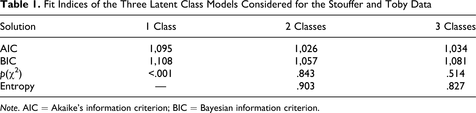
Note. AIC = Akaike’s information criterion; BIC = Bayesian information criterion.

Both results support the conclusion of Stouffer and Toby (1951), that “this fusion of variables in our situations does seem to generate a unidimensional scale, the dimension involved being the degree of strength of a latent tendency to be loyal to a friend even at the cost of other principles” (p. 400).

Summary and Outlook

The current article presents a free software, GANZ RASCH, which allows for parameter estimation and assessment of model fit of two important probabilistic models, the RM and the LCA (along with some support for the classical approach). One major focus was put on ease of use to facilitate the employment of the program for less experienced users. This goal is achieved through a GUI and an annotated output with some basic methodological hints concerning the procedures carried out. Therefore, the software might also be interesting for students of psychology, sociology, or educational science, for example.

The fit of both models can be judged by several criteria, each being sensitive to other kinds of model violation. Concerning the RM, special attention was paid to methods related to specific objectivity, because they are pivotal for the Rasch family of models. Item fit indices are provided as well, so many different users might find options he or she considers meaningful.

Of course, point-and-click software might entice users to apply methods they have not fully understood. Such an attitude shall not be befriended at all; therefore, clues and suggestions are integrated into the output annotations. They serve as teasers, providing incentives for exploring and dealing with the underlying theories. GANZ RASCH intends to offer a means of getting both acquainted with the RM and the LCA and of performing a full-fledged analysis.

Note that the program is continuously developed further, with new features emerging. Depending on the users’ comments and requests, specific features might be added in future versions. For keeping up with the newest development, the website www.ganzrasch.at will be maintained. GANZ RASCH can be obtained from this homepage or from the author via e-mail at no cost. Feedback of the users is very welcome, because it will result in further and targeted development of the software.

Footnotes

Acknowledgments

The author is indebted to Ingrid Koller for extensive program testing and invaluable debugging assistance under Windows, Marco J. Maier for testing the program under Linux, and Markus Schaer for testing the program under the MacOS.

Declaration of Conflicting Interests

The author declared no potential conflicts of interest with respect to the research, authorship, and/or publication of this article.

Funding

The author received no financial support for the research, authorship, and/or publication of this article.

Notes

References

Akaike

(1973). Information theory and an extension of the maximum likelihood principle. In Petrov

B. N.

Csáki

(Eds.), 2nd International Symposium on Information Theory (pp. 267–281). Budapest: Akademiai Kiádo.

Andersen

E. B.

(1970). Asymptotic properties of conditional maximum likelihood estimators. Journal of the Royal Statistical Society B, 32, 283–301.

Andersen

E. B.

(1973). A goodness of fit test for the Rasch model. Psychometrika, 38, 123–140.

Andersen

E. B.

(1980). Discrete statistical models with social science applications. Amsterdam, Netherlands: North-Holland.

Anderson

D. R.

Burnham

K. P.

(2002). Model selection and multimodel inference. A practical information-theoretic approach. 2nd ed. New York, NY: Springer.

Baker

F. B.

Harwell

M. R.

(1996). Computing elementary symmetric functions and their derivatives: A didactic. Applied Psychological Measurement, 20, 169–192.

Baker

F. B.

Kim

S. H.

(2004). Item response theory. Parameter estimation techniques (2nd ed., revised and expanded). New York, NY: Marcel Dekker.

Bock

R. D.

Lieberman

(1970). Fitting a response model for n dichotomously scored items. Psychometrika, 35, 197–197.

Bozdogan

(1987). Model selection and Akaike’s Information Criterion (AIC): The general theory and its analytical extensions. Psychometrika, 52, 345–370.

10.

Cronbach

L. J.

(1951). Coefficient alpha and the internal structure of tests. Psychometrika, 16, 297–334.

11.

Dayton

C. M.

(1998). Latent class scaling analysis. Thousand Oaks, CA: SAGE.

12.

Dayton

C. M.

Macready

G. B.

(2007). Latent class analysis in psychometrics. In Rao

C. R.

Sinharay

(Eds.), Psychometrics (Vol. 26, pp. 421–446. Amsterday: Elsevier North-Holland.

13.

Dempster

A. P.

Laird

N. M.

Rubin

D. B.

(1977). Maximum likelihood from incomplete data via the EM algorithm (with discussion). Journal of the Royal Statistical Society B, 39, 1–38.

14.

Embretson

S. E.

Reise

S. P.

(2000). Item response theory for psychologists. Mahwah, NJ: Lawrence Erlbaum.

15.

Fischer

G. H.

(1974). Einführung in die Theorie psychologischer Tests. [Introduction to the Theory of Psychological Tests]. Bern, Switzerland: Huber.

16.

Fischer

G. H.

Formann

A. K.

(1972). An algorithm and a FORTRAN program for estimating the item parameters of the linear logistic test model (Research Bulletin No. 11). Vienna, Austria: Psychologisches Institut der Universität Wien.

17.

Formann

A. K.

(1981). Über die verwendung von items als teilungskriterium für modellkontrollen im modell von Rasch [On using items as split criteria for assessing model fit of the Rasch Model]. Zeitschrift für Experimentelle und Angewandte Psychologie, 28, 541–560.

18.

Formann

A. K.

(1983). Modelltests für das Rasch modell durch teilgruppenbildung mittels latent class analyse [Testing the Rasch model using split groups based on latent class analysis]. Zeitschrift für experimentelle und angewandte Psychologie, 33, 387–412.

19.

Formann

A. K.

(1984). Die Latent-Class-Analyse. Einführung in Theorie und Anwendung [Latent class analysis. Introduction to theory and application]. Weinheim: Beltz.

20.

Formann

A. K.

(1995). Linear logistic latent class analysis and the Rasch model. In Fischer

G. H.

Molenaar

(Eds.), Rasch models: Foundations, recent developments, and applications (pp. 239–255). New York, NY: Springer.

21.

Formann

A. K.

(2003). Latent class model diagnostics—A review and some proposals. Computational Statistics & Data Analysis, 41, 549–559.

22.

Freeman

M. F.

Tukey

J. W.

(1950). Transformations related to the angular and the square root. Annals of Mathematical Statistics, 21, 607–311.

23.

Glas

C. A. W.

(1988). The derivation of some tests for the Rasch model from the multinomial distribution. Psychometrika, 53, 525–546.

24.

Glas

C. A. W.

Verhelst

N. D.

(1995). Testing the Rasch model. In Fischer

G. H.

Molenaar

(Eds.), Rasch models: Foundations, recent developments, and applications (pp. 69–95). New York, NY: Springer.

25.

Gustafsson

J.-E.

(1980). A solution of the conditional estimation problem for long tests in the Rasch model for dichotomous items. Educational and Psychological Measurement, 40, 327–385.

26.

Guttman

(1950). The basis for scalogram analysis. In Stouffer

S. A.

Guttman

Suchman

E. A.

Lazarsfeld

P. F.

Star

S. A.

Clausen

J. A.

(Eds.), Measurement and prediction (pp. 60–90). Princeton, NJ: Princeton University Press.

27.

Hays

W. L.

(1994). Statistics. 5th ed. Belmont, CA: Wadsworth/Cengage Learning.

28.

Hurvich

C. M.

Tsai

(1989). Regression and time series model selection in small samples. Biometrika, 76, 297–307.

29.

Lazarsfeld

P. F.

(1950). The logical and mathematical foundation of latent structure analysis. In Stouffer

S. A.

Guttman

Suchman

E. A.

Lazarsfeld

P. F.

Star

S. A.

Clausen

J. A.

(Eds.), Measurement and prediction (pp. 362–412). Princeton, NJ: Princeton University Press.

30.

McLachlan

G. J.

Krishnan

(1997). The EM algorithm and extensions. New York, NY: Wiley.

31.

Molenaar

(1983). Some improved diagnostics for failure of the Rasch model. Psychometrika, 48, 49–72.

32.

Molenaar

(1995). Estimation of item parameters. In Fischer

G. H.

Molenaar

(Eds.), Rasch models: Foundations, recent developments, and applications (pp. 39–51). New York, NY: Springer.

33.

Neyman

Scott

E. L.

(1948). Consistent estimates based on partially consistent observations. Econometrica, 16, 1–32.

34.

Parsons

(1949). Essays in sociological theory. Glencoe, IL: Free Press.

35.

Rasch

(1960). Probabilistic models for some intelligence and attainment tests. Studies in mathematical psychology I. Copenhagen: Danmarks Pædagogiske Institute.

36.

Rasch

(1966). An individualistic approach to item analysis. In Lazersfeld

P. F.

Henry

N. W.

(Eds.), Readings in mathematical social science (pp. 89–108). Cambridge, MA: MIT. Press.

37.

Ramaswamy

Desarbo

W. S.

Reibstein

D. J.

Robinson

W. T.

(1993). An empirical pooling approach for estimating marketing mix elasticities with PIMS data. Marketing Science, 12, 103–124.

38.

Read

T. R. C.

Cressie

N. A. C.

(1988). Goodness of fit statistics for discrete multivariate analysis. New York, NY: Springer.

39.

Sakamoto

Ishiguro

Kitagawa

(1986). Akaike information criterion statistics. Dordrecht, Netherlands: Reidel.

40.

Schwarz

(1978). Estimating the dimension of a model. The Annals of Statistics, 6, 461–464.

41.

Stouffer

Toby

(1951). Role conflict and personality. Journal of Sociology, 56, 395–406.

42.

Timminga

Adema

J. J.

(1995). Test construction from item banks. In Fischer

G. H.

Molenaar

(Eds.), Rasch models: Foundations, recent developments, and applications (pp. 111–127). New York, NY: Springer.

43.

. In van der Linden

W. J.

Glas

C. A. W.

(Eds.), Elements of adaptive testing. New York, NY: Springer.

44.

Warm

T. A.

(1989). Weighted likelihood estimation of ability in item response models. Psychometrika, 54, 427–450.

45.

Wilks

S. S.

(1938). The large-sample distribution of the likelihood ratio for testing composite hypotheses. Annals of Mathematical Statistics, 9, 60–62.

46.

Wright

B. D.

Douglas

G. A.

(1977). Conditional versus unconditional procedures for sample-free item analysis. Educational and Psychological Measurement, 37, 573–586.

47.

Wright

B. D.

Masters

G. N.

(1982). Rating scale analysis. Chicago, IL: Mesa.

48.

Wright

B. D.

Stone

M. H.

(1979). Best test design. Chicago, IL: Mesa.

“GANZ RASCH”

Abstract

Keywords

Introduction

GANZ RASCH 1 : A New Program

Models and Algorithms

Selected Features Specific to GANZ RASCH

RM: Parameter estimation with the CML method

RM: Parameter estimation with the pairwise method

RM: Goodness of fit with the Andersen test

RM: Goodness of fit with the Martin-Löf test

RM: Alpha inflation when applying multiple goodness-of-fit tests

Worked Examples

Example 1: The RM

Example 2: The Latent Class Model

Summary and Outlook

Footnotes

Acknowledgments

Declaration of Conflicting Interests

Funding

Notes

References

GANZ RASCH¹: A New Program