MRI classification and discrimination of spinal schwannoma and meningioma based on deep learning

Abstract

Backgroud:

Schwannoma (SCH) and meningiomas (MEN) are the two most common primary spinal cord tumors. Differentiating between them preoperatively remains a clinical challenge due to the substantial overlap in their clinical presentation and imaging characteristics.

Objective:

The objective of this study is to facilitate early diagnosis of patients and reduce clinician stress by constructing a deep learning-based classification model for automatic diagnosis of schwannoma and meningiomas using magnetic resonance images (MRI).

Methods:

We retrospectively collected MRI images of 74 patients with pathologically confirmed schwannoma and meningiomas from 2015 to 2020 at a local hosipital, and constructed a CNN model based on the PyTorch's deep learning framework for the discrimination between the two. First, a modified feature fusion CNN model (ResNet34-SKConv) was trained by introducing a selective convolutional kernel module into the original CNN model. The introduction of the selective convolutional kernel module enhances the network's focus on tumor features and effectively improves the network's performance. Finally, the trained model was used to process all the MRI image slices to achieve the classification of SCH and MEN patients by the voting prediction method.

Results:

Using the 5-fold cross-validation method, this new ResNet34-SKConv model achieves a classification accuracy of 92.32%, a specificity of 95.87%, and a F1-score of 93.54, respectively.

Conclusion:

This study demonstrated that a classification model using a deep learning network can be effective in achieving differential diagnosis of SCH and MEN. Thus, the new method has great potential for developing new computer-aided diagnosis and applications with future clinical practice.

Keywords

magnetic resonance imaging deep learning selective convolution kernel feature fusion spinal cord tumor

Introduction

With the trend of an aging society and the popularity of digital lifestyles, many people facing neck and shoulder pain and low back pain tend to first consider the common cervical spondylosis or lumbar disc herniation. However, among spinal cord diseases, spinal cord tumors are also an important cause of these symptoms. Spinal cord tumor is a general term for primary or secondary tumors occurring in the spinal cord and adjacent tissue structures (such as nerve roots, dura mater, adipose tissue and blood vessels, etc.). It is mainly divided into epidural and intradural tumors, and most of the epidural tumors are metastatic. Intradural spinal cord tumors can be further divided into extramedullary and intramedullary tumors. Primary spinal cord tumors are rare tumors in the Central Nervous System(CNS), accounting for 2%–4% overall,¹ and their incidence is one-tenth that of primary intracranial tumors.²In primary spinal cord tumors, the most common species include schwannoma (SCH) and meningioma (MEN).³ It is of paramount importance to distinguish between SCH and MEN preoperatively, as the treatment options for both are entirely distinct.

At present, clinicians and radiologists usually differentiate spinal tumors based on the imaging performance of Computed Tomography (CT) and Magnetic Resonance Imaging (MRI). Usually the vast majority of spinal cord tumors are soft tissue tumors, which show up on CT with a density very close to that of normal spinal cord tissue and nerve root tissue, making it difficult to distinguish spinal cord tumors on CT images. MRI has a higher resolution of soft tissue and allows for a clearer view of the location of spinal cord tumors in relation to the surrounding nerve tissue. On MRI imaging, SCH and MEN usually showed equal or slightly low signal on T1WI. On T2WI imaging, SCH and MEN showed high signal and slightly high signal, respectively. The T2WI signal within most SCH is not homogeneous and areas of higher signal cystic degeneration are seen, and punctate or irregular low signal is seen within MEN, which is due to the fact that SCH are susceptible to cystic deformation, whereas calcification often occurs within MEN.⁴ In terms of tumor morphology, necrotic cystic lesions were mostly seen within SCH; MEN was oval in shape, often with a spinal tail sign, and necrotic cystic lesions were rare. The spinal tail sign helps in the diagnosis of MEN, however, it is not present in all MEN and can still be confused with SCH in some cases.⁵ In terms of clinical manifestations, both present similarly with varying degrees of limb numbness, low back pain, segmental sensory deficits, and difficulty in urination and defecation,⁶ mainly due to compression of the spinal cord and nerve roots by the tumor. There are notable similarities between the two in terms of both clinical presentation and imaging. Consequently, the preoperative differentiation between SCH and MEN is clinically challenging.

Radiomics is a machine learning method for extracting quantitative imaging features from medical images in large quantities for medical image analysis.⁷ Its steps for differential diagnosis of spinal cord tumors include image data acquisition, image preprocessing, lesion segmentation, feature extraction and selection of spinal cord tumors, and finally classifier training and model evaluation. The purpose of image preprocessing is to remove noise and artifacts from the image, and to adjust the gray value range of the lesion image to make all the input images consistent for subsequent processing of the classification algorithm. Spinal cord tumor segmentation is to separate the tumor from the surrounding normal tissue, which is also called region of interest (ROI) segmentation. Most of this operation is performed manually by experienced clinicians, and the workload is heavy. The feature extraction algorithm mainly extracts feature information from spinal tumor images. Feature selection is to select the best features for the classification task using the feature selection algorithm. Finally, the tumor is classified using traditional machine learning classifiers. The commonly used classifiers include Support Vector Machine (SVM),⁸ k-Nearest Neighbor (KNN),⁹ Random forest (RF),¹⁰ logistic regression (LR),¹¹ etc. Garg et al.¹² used machine learning methods to develop a supervised classification model for spinal cord tumors and non-spinal cord tumors (normal), SVM, KNN, RF and LR methods were used to binary classify a set of pre-processed 180 non-tumor (normal) and 110 spinal cord tumors MRI image data. The experimental results showed that the performance of the RF model after 30 times cross-validation was optimization with an accuracy of 99.87%.

As a branch of machine learning, deep learning has shown great potential in the field of medical images. Compared with traditional machine learning algorithms, deep learning algorithms eliminate the need for manual delineation of the ROI, which can automatically learn features directly from the raw data, making the diagnosis process more efficient and accurate. Deep learning methods use network models to train a large amount of data, and can adaptively learn features to automatically extract tumor features, so as to judge the location and category of the tumors. At present, the application of deep learning in the differential diagnosis of spinal tumors is still in the preliminary stage. Zhuo et al.¹³ developed three two-classification models using two-dimensional Multi-ResUNet and DenseNet121 networks. The first classification model compared tumors with non-tumors using the Multi-ResUNet network, the second and third models used the DenseNet121 network for classifying spinal astrocytoma versus ventricular meningiomas, and multiple sclerosis versus optic neuromyelitis optica. Their model achieved 82% accuracy in distinguishing spinal astrocytoma from ventricular meningiomas, outperforming experienced neuroradiologists (72% accuracy). Ito et al.¹⁴ developed a system for automatic detection and classification of SCH and MEN based on deep learning, using the YOLO (You Only Look Once) the fourth version model. The classification accuracy of the MRI-based deep learning method for SCH and MEN on sagittal T1WI, T2WI, and T1WI combined T2WI images was 76.4%, 83.3%, and 84.1%, respectively, which exceeded the diagnostic accuracy of two spinal surgeons (77.4% and 76.1%, respectively).

A common challenge in medical imaging research is data scarcity, with few examples of publicly available annotated data. Deep learning generally requires a substantial amount of data for training. When addressing medical image classification problems, one often encounters the challenge of having a large network with too few clinical data samples to effectively train the model, resulting in overfitting. To mitigate the issue of limited data size in deep learning, techniques such as data augmentation¹⁵ and transfer learning¹⁶ can be employed. Data Augmentation typically uses operations such as flipping, rotating, panning, and scaling to synthesize modified data from the original data in order to increase the size of the dataset. The method of transfer learning can train ideal results even with small datasets, transfer learning plays an important role in deep learning classification tasks. Maki et al.¹⁷ used the methods of transfer learning and data augmentation to propose a convolutional neural network (CNN) based on Inception v3 network for MRI image classification of SCH and MEN. They used 2D slices of sagittal T1WI and T2WI as input to the network, achieving classification accuracies of up to 81%, which is comparable to experienced radiologists. Thus, the use of data augmentation strategies and transfer learning-based models can significantly improve the prognostic performance of typical small-sample medical imaging studies.

In addition to the studies using machine learning and deep learning models alone, there are studies that combine deep learning with clinical factors to establish multimodal models for differential diagnosis of tumors. Kita et al.¹⁸ combined CNN and TabNet to establish a bimodal network for the differential diagnosis of SCH and MEN in the spinal cord. They used sagittal T1WI images combined with clinical risk factors to bulid a bimodal model for the classification of SCH and MEN, achieving an accuracy of 83.5%.

Currently, the preoperative differential diagnosis of SCH and MEN is clinically important because spinal SCH and MEN are easily confused in clinical presentation as well as imaging, whereas the surgical options for the two are completely different. At this stage, there are few studies on MRI image classification based on deep learning for SCH and MEN, and the identification accuracy is not high enough. To address the above issues, we propose a deep learning based method for the classification of SCH and MEN. Our objective is to develop a CNN model for the classification of MRI images with the aim of distinguishing between SCH and MEN. Furthermore, we intend to perform a comprehensive evaluation of the performance of the CNN model for this classification. The main contributions of this study are summarized as follows:

We propose a deep learning classification model for MRI with SCH and MEN, which achieves accurate classification of SCH and MEN by voting prediction method.

Data augmentation techniques and transfer learning strategies are used. The data augmentation technique enriches and expands the original dataset to compensate for the lack of data and to improve the generalization ability of the model, and the transfer learning strategy is used in the training phase of the model so that the network performs well even with a limited amount of data.

We design a new feature fusion method. Selective Kernel Convolution (SKConv) is introduced into the model, and its output is multiplied element-by-element with the original input feature map, which effectively improves the classification performance of the network.

In the subsequent work, we evaluate and validate our proposed method, while introducing the Grad-Cam method for area visualization. Section 2 of the article provides a detailed description of the proposed method. Section 3 details the dataset construction and experimental setup. Section 4 analyzes the experimental results. Finally, the article is summarized in Section 5.

Methods

Figure 1 illustrates the workflow of the proposed overall classification model. Initially, the entire dataset is preprocessed. Subsequently, the dataset is partitioned into a training set and a testing set. The training set is then employed for network training through a five-fold cross-validation strategy and a transfer learning method. Each model weight is evaluated and validated. Ultimately, the lesions are predicted for each patient using the voting prediction method.

Figure 1.

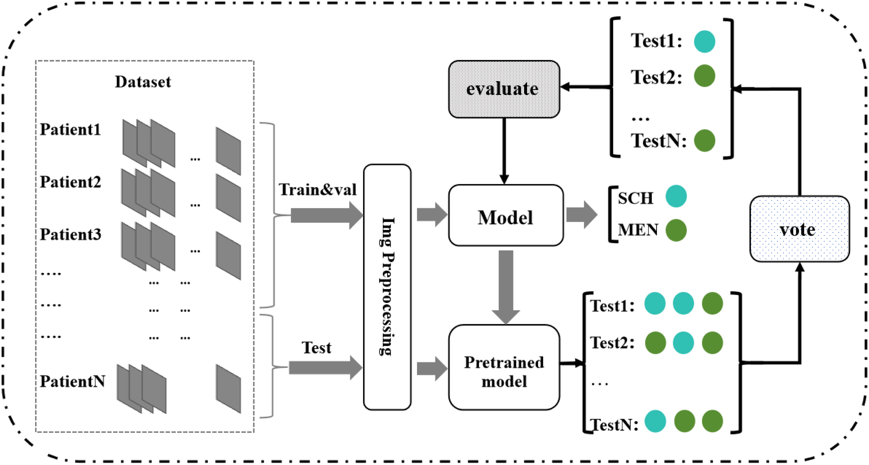
Diagram of overall flow.

Network architecture

In this study, we selected ResNet34¹⁹ as the backbone network for the classification task and fine-tuned the model using a transfer learning strategy. The pre-trained weights are obtained after training on the ImageNet dataset. The use of loading pre-training weights to implement the transfer learning strategy, which is conducive to the initialization of the model parameters, speeding up the training speed, and at the same time can improve the training effect of the model in the case of a small amount of data.²⁰The ResNet34 classification network structure is shown in Table 1 and Figure 2, which can be divided into backbone network layer and classification layer. The backbone network layer consists of: the first layer is 64 convolutions kernels of size 7*7 with a step size of 1, taking all-zero padding, and the activation function is ReLU function, the next layer connects the max-pooling layer with a step size of 2, and the next layer comprises 16 residual structures, each of which contains two convolution layers. In the classification layer, the feature map is first resized to 1 × 1 by a global average pooling operation, and then the feature map is downscaled by a linear layer and the final output is obtained.

Figure 2.

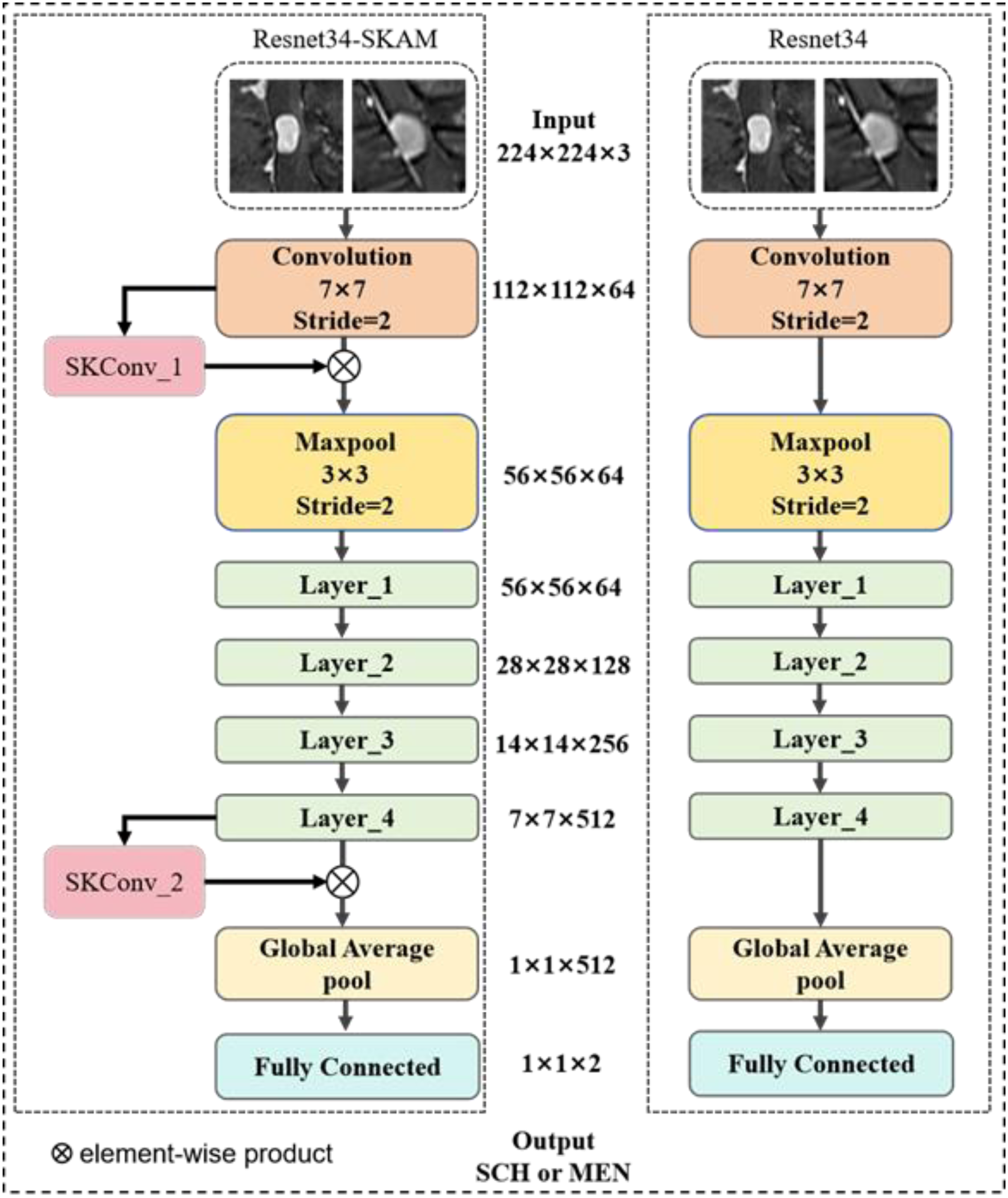
Diagram of network structure.

Table 1.

Network architecture of ResNet34.

Layer name	Output size	34-Layer
Conv	112 × 112	7 × 7,64,stride 2
Layer1	56 × 56	3 × 3maxpool,stride2
Layer1	56 × 56	$[\begin{matrix} 3 \times 364 \\ 3 \times 364 \end{matrix}] \times 3$
Layer2	28 × 28	$[\begin{matrix} 3 \times 3128 \\ 3 \times 3128 \end{matrix}] \times 4$
Layer3	14 × 14	$[\begin{matrix} 3 \times 3256 \\ 3 \times 3256 \end{matrix}] \times 6$
Layer4	7 × 7	$[\begin{matrix} 3 \times 3512 \\ 3 \times 3512 \end{matrix}] \times 3$
	1 × 1	average pool,40-d FC

Based on the above conditions, we introduce Selective Kernel Covlution (SKConv)²¹ in the backbone network, and the structure of Resnet34-SKConv network is shown in Figure 2.

Selective convolution kernel attention module

In convolutional neural networks, the size of the convolutional kernel is typically fixed, whereas the scale and size of real-world target objects may vary considerably. Consequently, a fixed convolutional kernel size may be unable to efficiently handle all situations. Inspired by the neuroscience community that neurons in the visual cortex adapt to receive and process information according to the size and intensity of the stimulus, we introduce a selective convolutional kernel module (SKConv) in the original backbone network. As illustrated in Figure 3, SKConv is a dynamic convolution operation that can adaptively adjust the size of the convolution kernel in accordance with the disparate spatial structures of the input data. This enables a more nuanced discovery of the correlation between the data features, thereby enhancing the recognition of the data. The implementation of SKConv can be divided into three steps: Split, Fuse, and Select.

Figure 3.

Structure of SKConv.

Split operation aims to generate branches with different sizes of convolution kernels. The input features are first passed through different convolutional kernels and processed to form two feature maps, which contain Convolution-Batch NorMalization-ReLU (CBR) units in the feature extraction process. These feature maps at different scales are stitched together to form a richer feature representation.

Fuse operation is a global representation that aggregates information from different branches to obtain selection weights. The procedure is to first sum the feature maps of all branches after the Split operation on an element-by-element basis, and then perform global average pooling on the summed results to compress the features to a global descriptor, followed by dimensionality reduction through a fully-connected layer to process the pooled features and generate channel descriptors at each scale, and then finally reshape the channel descriptors to the dimensions of the original inputs and normalize them by softmax normalization to generate weights for each scale.

Select operation is an element-by-element weighted fusion of the feature matrices of different branches to obtain the final feature map.

The channel attention mechanism is used in SKConv, which can automatically learn the importance of each channel. This mechanism allows the model to pay more attention to important features and suppress useless features, thus improving the performance of the model. Compared with the traditional convolutional kernel, SKConv is able to dynamically adjust the size of the sensory field, which can discover more correlations between data features, providing a better classification basis for the model to classify tumors of different sizes in the spinal cord. At the same time, SKConv has a deeper structure, and for simple feature maps, it only needs to build an ordinary network model to achieve the desired effect, so it also has the advantage of simplifying the model structure. The specific calculation processes of the aforementioned three operations are as follows:

Step 1 For task-given feature mapping $x \in R^{H \times W \times C}$ , first perform two transformations $\tilde{F} : x \to \tilde{U} \in R^{H \times W \times C}$ , $\hat{F} : x \to \hat{U} \in R^{H \times W \times C}$ , with different sizes of convolution kernels (e.g., 3 × 3 and 5 × 5), which are divided into $\tilde{U}$ and $\hat{U}$ .

Step 2 Secondly, sum $\tilde{U}$ and $\hat{U}$ element-wise to get $U$ : $U = \tilde{U} + \hat{U}$ . The channel statistics $s \in R^{C}$ are then generated by embedding the global information through global average pooling $F_{g p}$ , with c denoting the feature dimension of s :

s_{C} = F_{g p} (U_{C}) = \frac{1}{H \times W} \sum_{i = 1}^{H} \sum_{j = 1}^{W} U_{C} (i, j)

(1)

Step 3 Subsequently, the dimensionality is reduced by the fully connected layer

F_{f c}

to obtain

z \in R^{d \times 1}

z = F_{f c} (s) = δ (B (W s))

(2)

where

δ

is the ReLU function and ℬ denotes batch normalization,

W \in R^{d \times C}

Step 4 In order to study the impact of d (the number of feature dimensions after full connectivity, i.e., the number of feature dimensions of z) on the efficiency of the model, we use a reduction ratio r to control its value:

d = max (C / r, L)

(3)

where L denotes the minimal value of d and L = 32 is the default value.

Step 5 Finally, the weights a and b of each feature scale are obtained by Softmax and the convolved results are weighted and summed in Select.

We construct a new CNN model by introducing a selective convolutional kernel module (SKConv) into the original backbone network, adding it in front of the first layer of the backbone network as well as the classification layer, respectively, and applying an element-by-element feature fusion method by multiplying its output with the input feature map. By fusing features from the output of SKConv with the original input feature map, it helps the model to capture richer and more comprehensive features of spinal cord tumors. We experimentally validate the effectiveness of this feature fusion method in Section 3 and compare it with the feature fusion methods of other modules.

Voting prediction method

In the prediction stage, we adopt the voting prediction method, which mainly draws on the idea of hard voting in the voting mechanism, which means that each classifier outputs only one of the most probable category labels, and then votes based on these labels to select the category with the most votes as the final classification result. To assess the accuracy of the model predictions, this paper takes each patient as a whole, inputs all the slices of each patient's MRI image into the network for prediction, and votes on all the predictions for prediction. When the number of patient sections predicted to be SCH is greater than MEN, the patient is predicted to be SCH, otherwise the patient is predicted to be MEN. In clinical practice, radiologists tend to be more concerned about the sensitivity of tumor detection than the specificity. Therefore when the number of SCH was equal to MEN, we predicted it as SCH.

The calculation formula is presented in (3) : assuming that a patient has N slices, and the model predicts $c i (i = 1, 2, . . N)$ for each slice, resulting in the final prediction C.

C = a r g m a x (\sum_{i = 1}^{N} δ (c i = C j))

(4)

where

j = 1, 2, . ., K

, K is the total number of categories (here K takes 2), and

δ

is the indicator function. It takes the value 1 if

c i

is equal to

C j

and 0 otherwise.

Grad-CAM

In order to improve the interpretability of the model. We use Gradient-weighted Class Activation Mapping(Grad-CAM)^22,23 to visualize important regions or features for model decisions. Grad-CAM computes the activation map of the CNN on the input image by leveraging gradient information, and the color of the activation map can be utilized to indicate the degree of attention allocated to each component of the original image. The color red represents a higher weight value, indicating that the network pays more attention to the region. The color yellow represents the second-highest attention value, indicating that the model pays less attention to the region. The color blue represents the least attention value, indicating that the region is considered redundant information.

The principle of Grad-CAM is as follows: First compute $α_{k}^{c}$ , denotes the backpropagation of the prediction score $y^{c}$ through the prediction category c. The gradient information propagated onto the feature layer is then used to calculate the importance of each channel k of the feature layer A using the following formula:

α_{k}^{c} = \frac{1}{Z} \sum_{i} \sum_{j} \frac{\partial y^{c}}{\partial A_{i j}^{k}}

(5)

where

A_{i j}^{k}

denotes the feature layer A in channel k with coordinates of the data at position i (width), j (height), and Z denotes the number of pixels in the feature map, i.e., the width of the feature layer multiplied by the height.

Grad-CAM calculates the weighted sum of each channel in feature layer A by using ReLU activation function, and the calculation formula is as follows:

L_{G r a d - C A M}^{c} = Re LU (\sum_{k} α_{k}^{c} A^{k})

(6)

Where A represents a certain feature layer (generally the last convolutional layer output is taken), k represents the kth channel in the feature layer A, c represents the category of interest,

A^{k}

represents the data of channel k in the feature layer A, and

α_{k}^{c}

represents the weight of the category c in the kth channel of the feature layer A for the category.

Experiments

Dataset and preprocess

The data for this study were retrospectively collected from 74 patients with spinal cord SCH and MEN at a local hospital between 2015 and 2020. The age range of the patients was 17 to 84 years old. A total of 41 patients were diagnosed with SCH, while 33 patients were diagnosed with MEN, as indicated by the pathological reports. Inclusion criteria: (1) All tumor MRI images were obtained prior to any therapeutic intervention; (2) The MRI imaging data for all patients included sagittal planar (T1 W) enhancement sequences, and the tumors were classified as primary intradural extramedullary; and (3) The clinical and pathological data were complete. The exclusion criteria are as follows: (1) The quality of the MRI images was suboptimal, with artifacts or insufficient sharpness; (2) the MRI images of each sequence scan were incomplete.

The data contained 41 SCH and 33 MEN patients. Consistent with previous studies, we chose sagittal slices for the classification experiment. Sagittal sections can clearly show the anteroposterior relationship between the spinal cord and surrounding tissues. This is essential for assessing the location and size of spinal cord tumors and their impact on surrounding structures; the T1WI enhancement sequences of MRI were selected as the network input images, and there were 2–4 slices of each patient's T1WI enhancement sequences that contained the part of the tumor, with a total of 127 slices for SCH and 89 slices for MEN; the MRI images of the two patients are shown in Figure 4. In the image preprocessing stage we took the 3D images in Dicom format and firstly cropped them in 3D by 3D-Slicer software, the cropping criterion was the smallest area containing the anterior and posterior boundaries of the tumor and the spinal canal, and saved them in the nii format, and then adjusted the window width and window position of all the patients’ slices using the itk-snap software and converted them to the png format. In order to solve the problem of insufficient data volume and imbalance, we made the following efforts: we expanded the size of the dataset (while preserving the original data) by using seven data augmentation techniques on the original data, using the following: image rotation by 30°, a wide shift range of 0.2, a high shift range of 0.2, a luminance range of 0.5–0.9, a shear range of 0.1, a zoom range of 0.2, and a horizontal flip. Finally we get SCH 1016 images and MEN 712 images. Finally, we uniformly resized all images to 224 × 224 and normalized them by dividing each pixel by 255 to keep the pixel values in the 0–1 range before feeding them into the network.

Figure 4.

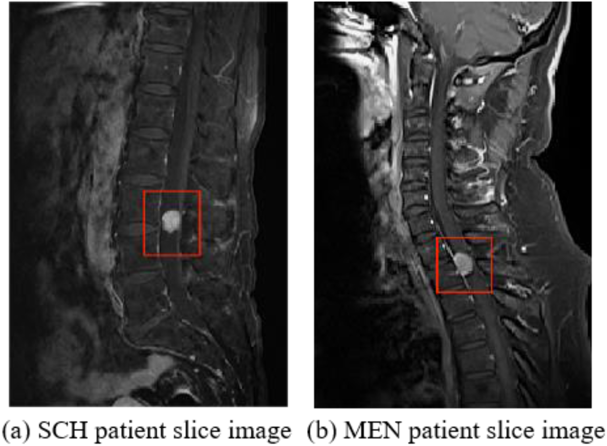
Example images of sections from patients with different intraspinal tumors.

In order to verify the stability and reproducibility in the training of the model, this experiment uses a five-fold cross-validation strategy. Firstly, the dataset is randomly divided into a training set and a test set in the ratio of 8:2 in terms of patients. During the training process, the training set is divided into 5 equal parts according to the number of categories, and one of them is selected as the validation set during each training, and the remaining part is used as the training set, and the training is repeated for 5 times. The weight result files obtained after 5 times of training are evaluated in the test set for the model respectively, and the average of the obtained results is the overall performance of the model.

Evaluation metrics

In order to evaluate the performance of the proposed model, five evaluation metrics are introduced: accuracy (ACC), sensitivity (SEN), specificity (SPE), precision rate (PRE), and F1-score (F1), which are given below:

A C C = \frac{T P + T N}{T P + F P + T N + F N}

(7)

S E N = \frac{T P}{T P + F N}

(8)

S P E = \frac{T N}{F P + T N}

(9)

P R E = \frac{T P}{T P + F P}

(10)

F 1 = \frac{2 T P}{2 T P + F N + F P}

(11)

where TP represents true positive, FP represents false positive, TN represents true negative and FN represents false negative. In calculating these metrics, we consider SCH as a positive category.

Implementation details

In this experiment, all models are loaded with pre-training weights, which allows the network to be fitted better and speeds up the training process. In the hyperparameter settings, epochs were set to 50 and batchsize size was set to 16. The model input size was 224 × 224 pixels. The Adam optimizer was used, the initial learning rate was set to 0.0004 and decayed every 5 epochs to 0.9. In CAM, SKConv attention mechanism, the channel attention compression ratio was set to 16. All the experiments were carried out in the PyTorch framework under Widows11 system and accelerated training was performed under RTX 4060 ti16GB.

In our experiments we used the cross-entropy loss function as the loss function of the experiment. The calculation formula is shown below:

L_{C E} = - \sum_{i = 1}^{2} y_{i} \log (P i)

(12)

where i has a value range of 1–2, denotes two categories, denotes the underlying fact, and

P i

denotes the predicted probability. All indicators are calculated based on cases (patients).

Results and discussion

Ablation experiments

Firstly, we compare the classification performance of the model without transfer learning and after using the transfer learning method. We use ResNet34 as the baseline network. The results are shown in Table 2, which presents the findings from the five-fold cross-validation method. It is evident that the application of the transfer learning strategy has led to a notable enhancement in the performance of ResNet34, with an observed increase in accuracy by 8.58%. The results demonstrate the efficacy of transfer learning in enhancing model performance.

Table 2.

Comparison of results of ablation experiment and different attention modules.

Networks	ACC(±SD,%)	SPE(%)	SEN(%)	PRE(%)	F1(%)
ResNet34(No transfer learning)	80.53(±5.43)	78.76	82.24	84.06	83.04
ResNet34	89.11(±1.18)	89.18	90.09	91.56	90.55
ResNet34 + CBAM	90.71(±3.12)	94.88	88.7	96.25	92.21
ResNet34 + CAM	91.61(±1.65)	86.86	96.87	88.44	92.26
ResNet34 + SENet	89.64(±1.65)	87.20	93.35	89.06	90.76
ResNet34 + ECA	89.82(±1.55)	90.05	90.11	92.50	91.18
ResNet34 + CA	91.07(±1.70)	87.47	95.08	89.38	91.90
ResNet34 + SKConv (Ours)	92.32(±1.07)	95.87	90.20	97.19	93.54

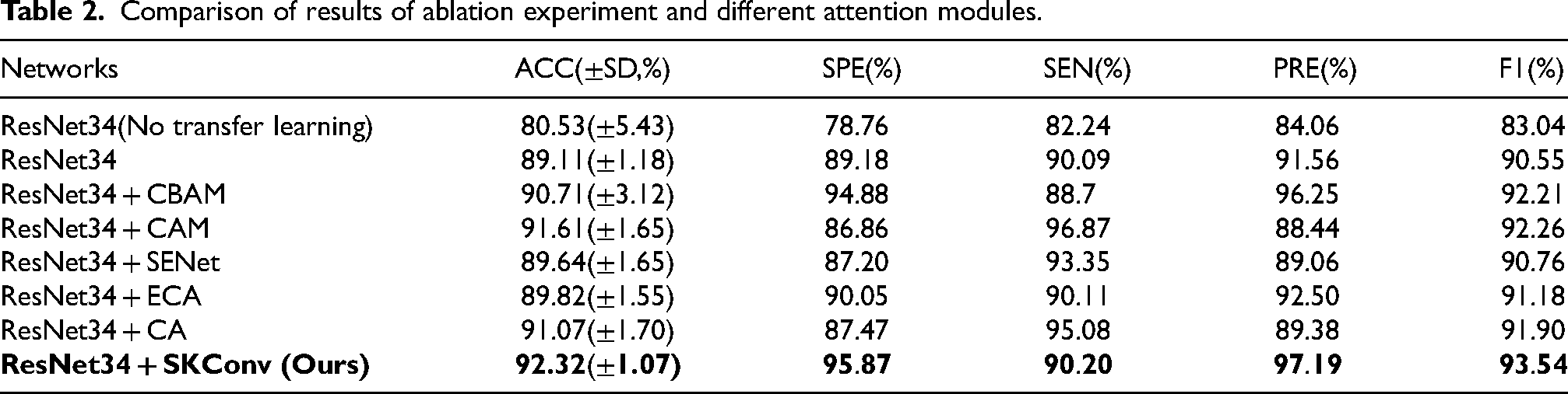
Secondly, as the channel attention mechanism is employed in the SKConv module, we undertake a comparative analysis of the introduction of distinct channel attention mechanism modules within the ResNet34 model, adopting a consistent feature fusion approach in alignment with that of SKConv. A comparison is made of the classification performance after the introduction of the CAM, SENet,²⁵ CA,²⁶ ECA²⁷ and SKConv modules. CAM represents the channel attention module in CBAM.²⁴ SE, ECA, and CA are representative channel attention mechanisms.

The addition of CAM improves the classification accuracy and F1 index of the model by 2.5% and 1.71%, respectively, compared to the baseline network; the addition of SENet, ECA, and CA improves the model accuracy and F1 by 0.53% and 0.21%, 0.71 and 0.63%, and 1.96% and 1.35%, respectively; and lastly, the addition of SKConv improves the model accuracy and F1 by 3.21% and 2.99%, which is a substantial performance improvement.

Through the above ablation experiments, we conclude that the feature fusion model (ResNet34-SKConv), which uses the transfer learning method and introduces the SKConv module, has the best classification accuracy and stable results. In the next experiments, we choose the above settings in both network structure and modules.

Effectiveness of feature fusion

Since the traditional approach to improve the network is to directly input the original input feature map into the attention module and then use the output of the attention module as the final features. However, this approach has some limitations in capturing the complex relationships between input features, as it may not adequately take into account the importance and correlation between different features. Since SCH and MEN often have insignificant differences in image presentation, in order to better identify these two types of tumors that are easily confounded for diagnosis, we designed a new feature fusion method that dynamically adjusts the importance of each original input feature map using the SKConv module. Specifically, we achieved fine control over the interaction between different tumor features by multiplying the output of the SKConv module with the original input feature maps element by element. This strategy enables the model to integrate and utilize the correlation information between input features more effectively, enhances the network's sensitivity to subtle feature changes in the input feature maps, and thus significantly improves the accuracy and performance in the spinal cord tumor classification task.

In order to verify the effectiveness of the feature fusion method with the original input feature map after introducing SKConv, this experiment compares the classification performance of the model without feature fusion, and the results are shown in Table 3. It can be seen that the classification accuracy of the model after feature fusion with the original input feature map is improved by 0.89% compared with the model without feature fusion, which indicates the effectiveness of our proposed feature fusion method.

Table 3.

Comparison results with the method without feature fusion.

Network	ACC(±SD,%)	SPE(%)	SEN(%)	PRE(%)	F1(%)
ResNet34 + SKConv(Feature-free fusion)	91.43(±0.91)	95.36	89.50	96.56	92.78
ResNet34 + SKConv (Ours)	92.32(±1.07)	95.87	90.20	97.19	93.54

In order to further demonstrate the regions that the model pays attention to the images after adding the SKConv module, 2 sets of MRI images containing SCH and MEN were selected for Grad-Cam visualization in the experiment. The results are shown in Figure 5, where it can be shown that the ResNet34-SKConv model with only the addition of the selective convolutional kernel attention mechanism has a more accurate level of attention to the lesion region.

Figure 5.

Grad-Cam map of different attention.

Comparison experiment with traditional CNN

In order to compare ResNet34-SKConv with traditional CNN models, we compared four models, VGG16,²⁸ ResNet50,¹⁹ InceptionV3,²⁹ and DenseNet121.³⁰ All models use the transfer learning strategy with the same parameter settings as in Section 3.3. As shown in Table 4, where VGG16 has a relatively low classification accuracy due to its stacking approach and lack of feature extraction ability. ResNet50 has more layers and parameters compared to ResNet34, resulting in a lower classification accuracy for small sample tasks using the relatively complex ResNet50. Similarly, InceptionV3 and DenseNet121 do not have as good classification accuracy as the structurally simple ResNet34 in dealing with relatively simple binary classification tasks due to their more complex models and deeper layers compared to ResNet34. From the specific data results in Table 4, we can learn that our proposed ResNet34-SKConv has the best classification performance.

Table 4.

Results of comparion experiment.

Networks	ACC(±SD, %)	SPE(%)	SEN(%)	PRE(%)	F1(%)
VGG16	75.71(±3.85)	76.41	77.96	82.5	79.31
ResNet50	83.57(±2.86)	89.57	81.28	93.13	86.61
InceptionV3	84.82(±2.26)	87.63	84.63	90.63	87.12
DenseNet121	86.43(±2.49)	87.48	88.54	89.06	88.10
ResNet34	89.11(±1.18)	89.18	90.09	91.56	90.55
ResNet34 + SKConv (Ours)	92.32(±1.07)	95.87	90.20	97.19	93.54

Discussion

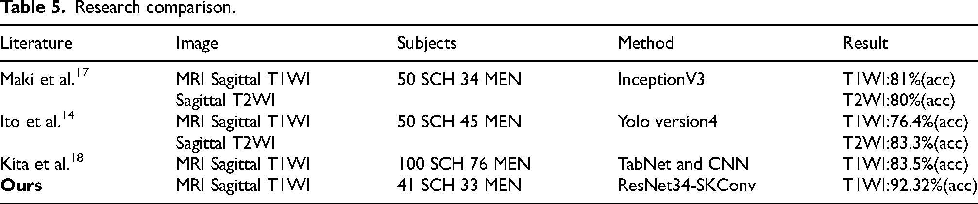
Table 5 presents a comparison of the classification results obtained using the proposed method and those reported in previous studies. Maki et al.¹⁷ used transfer learning and data augmentation to propose a CNN based on Inception v3 network for classification of MRI images of SCH and MEN, using 2D slices of sagittal T1WI and T2WI as input to the network, with a classification accuracy of up to 81%. Ito et al.¹⁴ developed a deep learning-based system for automatic detection and classification of SCH and MEN using the YOLO (You Only Look Once) version 4 model. The accuracy of the MRI-based deep learning method for classification of SCH and MEN in sagittal T1WI, T2WI, and T1WI combined with T2WI was 76.4%, 83.3%, and 84.1%, respectively. These results exceeded the diagnostic accuracy of two spine surgeons (accuracy of 77.4% and 76.1%, respectively). In a study by Kita et al.,¹⁸ a convolutional neural network (CNN) and TabNet were combined to create a bimodal network for the differential diagnosis of SCH and MEN. This model was developed using sagittal T1-weighted imaging (T1WI) and clinical risk factors, and achieved an accuracy of 83.5% in classifying SCH and MEN. In comparison to previous studies, this paper presents a classification model that is capable of differentiating between spinal cord SCH and MEN. Additionally, it introduces Grad-Cam for the visualization of the model's ROI. The final experimental results demonstrate that the proposed model exhibits an accuracy, specificity, sensitivity, and F1-score of 92.32%, 95.87%, 90.20%, 97.19%, and 93.54%, respectively, which signifies a notable degree of classification efficacy.

Table 5.

Research comparison.

Literature	Image	Subjects	Method	Result
Maki et al.¹⁷	MRI Sagittal T1WISagittal T2WI	50 SCH 34 MEN	InceptionV3	T1WI:81%(acc)T2WI:80%(acc)
Ito et al.¹⁴	MRI Sagittal T1WISagittal T2WI	50 SCH 45 MEN	Yolo version4	T1WI:76.4%(acc)T2WI:83.3%(acc)
Kita et al.¹⁸	MRI Sagittal T1WI	100 SCH 76 MEN	TabNet and CNN	T1WI:83.5%(acc)
Ours	MRI Sagittal T1WI	41 SCH 33 MEN	ResNet34-SKConv	T1WI:92.32%(acc)

There are some restrictions to this study. Primarily, it is a retrospective, single-center study with a relatively small sample size. To ensure the reliability and generalizability of the findings, a multicenter study with a larger sample size is necessary for internal and external validation. This is crucial for future clinical applications. Secondly, only slices of T1WI enhancement sequences of MRI were classified in this study, and multi-sequence and multi-modality imaging methods can be further explored in the future to improve the accuracy. In future research work, if more relevant data can be collected, the identification accuracy of the classification modeling system can be improved by combining images from coronal and axial sequences.

Conclusion

Preoperative discrimination between SCH and MEN remains a clinical challenge. In this study, we propose ResNet34-SKConv based on CNN architecture for computer-aided differential diagnosis of SCH and MEN in spine MRI scans. Compared to previous studies, our proposed classification model introduces a selective convolutional kernel module and designs a new feature fusion method: the output of the module is multiplied element-by-element with the original input feature map. In the experiments, a transfer learning strategy is employed. The pre-trained weights are used to initialize the weights in order to speed up the convergence of the model. The data augmentation we use in the data preprocessing phase plays a key role in optimizing the model performance: the original smaller dataset can be enriched by expanding it using techniques such as random transformations, flipping and scaling. Better results were achieved with a total of 1728 MRI slices of spinal cord tumors obtained after eightfold data augmentation expansion in 74 patients. Experimental results show that our proposed model demonstrates excellent classification results in sagittal T1WI-enhanced slices of MRI from SCH and MEN, with an accuracy of 92.32%, precision of 95.87%, and sensitivity of 90.20%, which outperforms most of the existing deep-learning-assisted diagnostic methods.

In summary, consistent with previous studies, the MRI-based deep learning classification framework can be used as a new medical image analysis method for preoperative differentiation between SCH and MEN with good diagnostic performance, which is expected to optimize the treatment plan and avoid unnecessary surgeries, and finally, further studies are needed to confirm the validity of our conclusions. In the future, a series of automated methods such as automatic identification of desired regions and classification can also be realized using target detection techniques.

Footnotes

ORCID iD

Yuanjun Wang

Funding

The authors received no financial support for the research, authorship, and/or publication of this article.

Declaration of conflicting interests

The authors declared no potential conflicts of interest with respect to the research, authorship, and/or publication of this article.

References

Abd-El-Barr

Huang

Moses

, et al. Recent advances in intradural spinal tumors. Neuro-oncol 2018; 20: 729–742.

Grimm

Chamberlain

. Adult primary spinal cord tumors. Expert Rev Neurother 2009; 9: 1487–1495.

Puac-Polanco

Guarnizo

Cruz

, et al. Intradural extramedullary tumors and associated syndromes. Neuroimaging Clin 2023; 33: 407–422.

Liu

Zhang

, et al. MRI Diagnosis of intradural extramedullary tumors. J Cancer Res Ther 2014; 10: 927–931.

Liu

Choi

Lee

, et al. Radiological findings of spinal schwannomas and meningiomas: focus on discrimination of two disease entities. EurRadiol 2009; 19: 2707–2715.

Chamberlain

Tredway

. Adult primary intradural spinal cord tumors: a review. Curr Neurol Neurosci Rep 2011; 11: 320–328.

Zhang

, et al. Deep learning with radiomics for disease diagnosis and treatment: challenges and potential. Front Oncol 2022; 12: 773840.

Zhang

. Support vector machine classification algorithm and its application. In: Information computing and applications: Third international conference, ICICA 2012, Chengde, China, September 14–16, 2012. Proceedings, Part II 3, 2012, pp.179–186.

Cover

Hart

. Nearest neighbor pattern classification. IEEE Trans Inf Theory 1967; 13: 21–27.

10.

Breiman

. Random forests. Machine Learning 2001; 45: 5–32.

11.

Zhang

. Model building strategy for logistic regression: purposeful selection. Ann Transl Med 2016; 4: 111.

12.

Garg

Raghavan

. Comparison of machine learning algorithms for the classification of spinal cord tumor. Irish J Med Sci (1971–) 2024; 193: 571–575.

13.

Zhuo

Zhang

Duan

, et al. Automated classification of intramedullary spinal cord tumors and inflammatory demyelinating lesions using deep learning. Radioly: Artif Intell 2022; 4: e210292.

14.

Ito

Nakashima

Segi

, et al. Automated detection and diagnosis of spinal schwannomas and meningiomas using deep learning and magnetic resonance imaging. J Clin Med 2023; 12: 5075.

15.

Krizhevsky

Sutskever

Hinton

. Imagenet classification with deep convolutional neural networks. Commun ACM 2017; 60: 84–90.

16.

Zhou

Zhang

WANG

, et al. Transfer learning and its application research. J Phys: Conf Ser 2021; 1920: 012058.

17.

Maki

Furuya

Horikoshi

, et al. A deep convolutional neural network with performance comparable to radiologists for differentiating between spinal schwannoma and meningioma. Spine 2020; 45: 694–700.

18.

Kita

Fujimori

Suzuki

, et al. Bi-modal network combining convolutional neural network and TabNet, differentiating spinal tumors based on images and clinical risk factors. In: Medical imaging 2023: Computer-aided diagnosis, Vol.12465, 2023.

19.

Zhang

Ren

, et al. Deep residual learning for image recognition. In: Proceedings of the IEEE conference on computer vision and pattern recognition 2016, pp.770–778.

20.

Gupta

Pathak

Kumar

. Deep learning (CNN) and transfer learning: a review. J Phys: Conf Ser 2022; 2273: 012029.

21.

Wang

, et al. Selective kernel networks. In: Proceedings of the IEEE/CVF conference on computer vision and pattern recognition 2019, pp.510–519.

22.

Selvaraju

Cogswell

Das

, et al. Grad-cam: visual explanations from deep networks via gradient-based localization. In: Proceedings of the IEEE international conference on computer vision 2017, pp.618–626.

23.

Selvaraju

Das

Vedantam

, et al. Grad-CAM: why did you say that?, arxiv preprint arxiv:1611.07450 (2016).

24.

Woo

Park

Lee

, et al. Cbam: convolutional block attention module. In: Proceedings of the European conference on computer vision (ECCV) 2018, pp.3–19.

25.

Shen

Sun

. Squeeze-and-excitation networks. In: Proceedings of the IEEE conference on computer vision and pattern recognition 2018, pp.7132–7141.

26.

Hou

Zhou

Feng

. Coordinate attention for efficient mobile network design. In: Proceedings of the IEEE/CVF conference on computer vision and pattern recognition 2021, pp.13713–13722.

27.

Wang

Zhu

, et al. ECA-net: efficient channel attention for deep convolutional neural networks. In: Proceedings of the IEEE/CVF conference on computer vision and pattern recognition 2020, pp.11534–11542.

28.

Simonyan

Zisserman

. Very deep convolutional networks for large-scale image recognition, arxiv preprint arxiv: 1409.1556 (2014), 1–14.

29.

Szegedy

Vanhoucke

loffe

, et al. Rethinking the inception architecture for computer vision. In: Proceedings of the IEEE conference on computer vision and pattern recognition 2016, pp.2818–2826.

30.

Huang

Liu

Van Der Maaten

, et al. Densely connected convolutional networks. In: Proceedings of the IEEE conference on computer vision and pattern recognition 2017, pp.4700–4708.