A study on CT detection image generation based on decompound synthesize method

Abstract

Background:

Nuclear graphite and carbon components are vital structural elements in the cores of high-temperature gas-cooled reactors(HTGR), serving crucial roles in neutron reflection, moderation, and insulation. The structural integrity and stable operation of these reactors heavily depend on the quality of these components. Helical Computed Tomography (CT) technology provides a method for detecting and intelligently identifying defects within these structures. However, the scarcity of defect datasets limits the performance of deep learning-based detection algorithms due to small sample sizes and class imbalance.

Objective:

Given the limited number of actual CT reconstruction images of components and the sparse distribution of defects, this study aims to address the challenges of small sample sizes and class imbalance in defect detection model training by generating approximate CT reconstruction images to augment the defect detection training dataset.

Methods:

We propose a novel CT detection image generation algorithm called the Decompound Synthesize Method (DSM), which decomposes the image generation process into three steps: model conversion, background generation, and defect synthesis. First, STL files of various industrial components are converted into voxel data, which undergo forward projection and image reconstruction to obtain corresponding CT images. Next, the Contour-CycleGAN model is employed to generate synthetic images that closely resemble actual CT images. Finally, defects are randomly sampled from an existing defect library and added to the images using the Copy-Adjust-Paste (CAP) method. These steps significantly expand the training dataset with images that closely mimic actual CT reconstructions.

Results:

Experimental results validate the effectiveness of the proposed image generation method in defect detection tasks. Datasets generated using DSM exhibit greater similarity to actual CT images, and when combined with original data for training, these datasets enhance defect detection accuracy compared to using only the original images.

Conclusion:

The DSM shows promise in addressing the challenges of small sample sizes and class imbalance. Future research can focus on further optimizing the generation algorithm and refining the model structure to enhance the performance and accuracy of defect detection models.

Keywords

CT detection image generation decompound synthesize method (DSM)contour-CycleGAN copy-Adjust-Paste(CAP)

Introduction

Nuclear graphite and carbon components are essential structural elements in the cores of high-temperature gas-cooled reactors(HTGR), serving functions such as neutron reflection, moderation, and insulation.¹ Since these components cannot be replaced throughout the reactor's lifetime once installed, their quality is critical to the structural safety and stable operation of the reactors. Therefore, volumetric inspection of internal defects in graphite and carbon components during production is crucial for ensuring the safe operation of reactors and extending their service life.

Currently, there are no effective methods, either domestically or internationally, for batch inspection of internal defects such as holes, looseness, and cracks in large graphite and carbon components. Three-dimensional volumetric inspection remains a pressing challenge. Compared to traditional detection methods such as ultrasound and eddy current testing,² three-dimensional high-energy X/γ-ray non-destructive testing technology can simultaneously meet the requirements for large size, high spatial resolution, high density resolution, and high efficiency. Therefore, employing helical CT technology for internal defect detection in graphite and carbon components holds significant application potential.

However, due to the large number of internal components in reactors and the massive data volume generated from helical CT image reconstructions, manual visual inspection methods suffer from low detection efficiency, high rates of false positives and negatives, and place significant demands on the inspectors’ skills. In recent years, deep learning-based methods have made notable progress in the intelligent detection of defects in CT image, with convolutional neural networks (CNNs) particularly excelling in image processing.^3–5 Nevertheless, these methods heavily depend on large training datasets, making it challenging to effectively train models without sufficient samples. Acquiring actual CT reconstruction image samples, especially those containing defects, is difficult. Real defects vary greatly in shape and complexity, and different types of defects are unevenly distributed. These problems of small sample sizes and class imbalance pose significant challenges for training models using deep learning methods.

The small sample sizes problem refers to the limited number of defect-containing images available for training from reconstructed images of graphite and carbon components—currently only about 200 actual defect images. This small dataset can lead to model overfitting and insufficient generalization capability. Expanding the dataset is a direct way to address the small sample sizes problem, for example, data augmentation techniques such as random translation and rotation can be used to enlarge the sample set.^6–9 Additionally, transfer learning¹⁰ and meta-learning^11,12 methods can also be employed to mitigate this issue.

The class imbalance problem refers to the uneven distribution of different defect types within the training dataset for defect detection models.¹³ This imbalance can cause the model to perform inconsistently when detecting various types of defects, affecting both training and performance. The methods to address class imbalance include data augmentation, resampling, and algorithmic approaches such as sample weighting, threshold adjustment, and the use of Generative Adversarial Networks (GANs).^14,15

To address the problems of small sample sizes and class imbalance in CT image defect detection, the most direct solution is to expand the dataset by increasing the number of images and defect samples. Based on this approach, existing methods primarily utilize GANs¹⁶ and other image generation models. These models learn the distribution characteristics of existing image samples to generate synthetic images similar to actual CT reconstruction images. However, these methods often fail to fully account for the unique characteristics of CT images, making it challenging to generate realistic synthetic images that closely resemble actual defects (as shown in Figure 1). This can interfere with the recognition of real defects, thereby limiting the accuracy and robustness of defect detection models.

Figure 1.

Comparison between actual and simulated CT reconstructed images.

To address these challenges and improve the performance and generalization capabilities of CT image defect detection models, this paper introduces an innovative CT detection image generation algorithm based on component decomposition, termed the Decompound Synthesize Method (DSM). This method aims to construct a CT image defect detection dataset and effectively resolve the problems of small sample sizes and class imbalance. The main contributions and innovations of this paper include:

Component Decomposition: The DSM algorithm decomposes CT images into different components and uses targeted methods to generate approximate samples for each component, enhancing the realism and similarity of the generated images.

Sample Expansion: The DSM algorithm effectively expands the number of defect detection samples, addressing the small sample sizes problem and providing robust data support for improving the accuracy and reliability of CT image defect detection.

Defect Synthesis: By designing a rational generation algorithm and defect synthesis method, DSM produces synthetic images with defects similar to those in actual CT images. This approach is validated using real experimental data, demonstrating improved accuracy and robustness in defect detection models.

Methods

Actual CT defect detection images contain three main types of information: noise and artifacts, the background image, and various types of defects. To generate synthetic images that closely resemble actual CT reconstructions, expand the defect detection sample set, and address problems in image generation, we proposes a CT detection image generation algorithm based on component decomposition, termed the Decompound Synthesize Method (DSM). This algorithm decomposes CT images into different components and generates approximate samples for each, ultimately synthesizing images with realistic defect textures. This approach effectively expands the training dataset for defect detection, addressing the problems of small sample sizes and class imbalance. The overall workflow of the method is shown in Figure 2.

Figure 2.

Ct detection image generation algorithm DSM.

The proposed method consists of three main steps: model conversion, background generation, and defect synthesis.

Model Conversion: First, STL files of various industrial components are converted into voxel data. By performing forward projection and image reconstruction on the voxel data, we obtain reconstructed images corresponding to actual CT images.

Background Generation: Using an image generation model, synthetic images that closely resemble actual CT images are produced. The goal of this step is to generate images containing the base information but without defects.

Defect Synthesis: Defect samples are randomly sampled from an existing defect library and added to the images according to a predetermined method. This process generates realistic defect textures in the synthetic images, thereby increasing the number of defect samples.

Images generated using the DSM can be utilized for subsequent defect detection model training. Compared to artificial and unrealistic defect samples, those generated by this method closely resemble defects in actual CT images, thereby enhancing the accuracy of defect detection models in practical applications. The following sections provide a detailed description of each of the three steps.

Model conversion

Given that existing nuclear graphite and carbon components have relatively uniform shapes, it is essential to enhance the generalization ability of defect detection models to different shapes. To achieve this, we voxelized the vector files of industrial components to construct CT images with diverse shapes. As illustrated in Figure 3, an example of an industrial component demonstrates a wide variety of shapes and structures. First, we used the open-source tool stl2voxel¹⁷ to obtain binary voxel data for the component. Next, we performed forward projection and image reconstruction on the voxel data to incorporate potential features of actual reconstructed images. This process reduces differences in image characteristics and obtains reconstructed images that reflect the component's shape.

Figure 3.

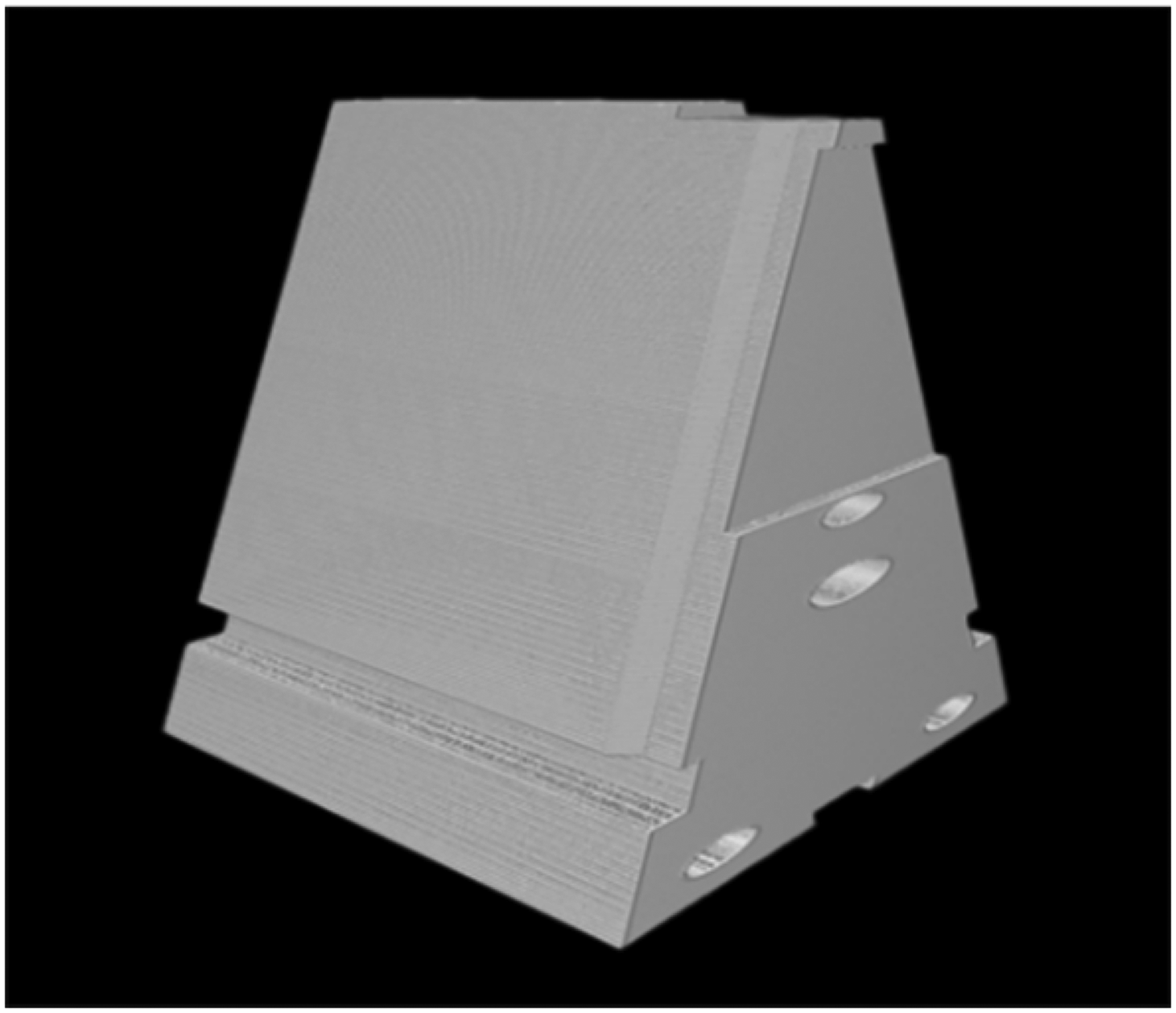
Schematic of an industrial component.

Although actual reconstructed images have undergone ring artifact removal, slight ring artifacts may still appear under certain conditions. To minimize differences between the generated CT images and actual CT images, we also introduced a small amount of ring artifacts into the generated images. The final generated image, as shown in Figure 4, exhibits more diverse shapes and contours, and includes a certain degree of reconstruction artifacts and ring artifacts, thereby achieving a higher degree of similarity to actual CT images.

Figure 4.

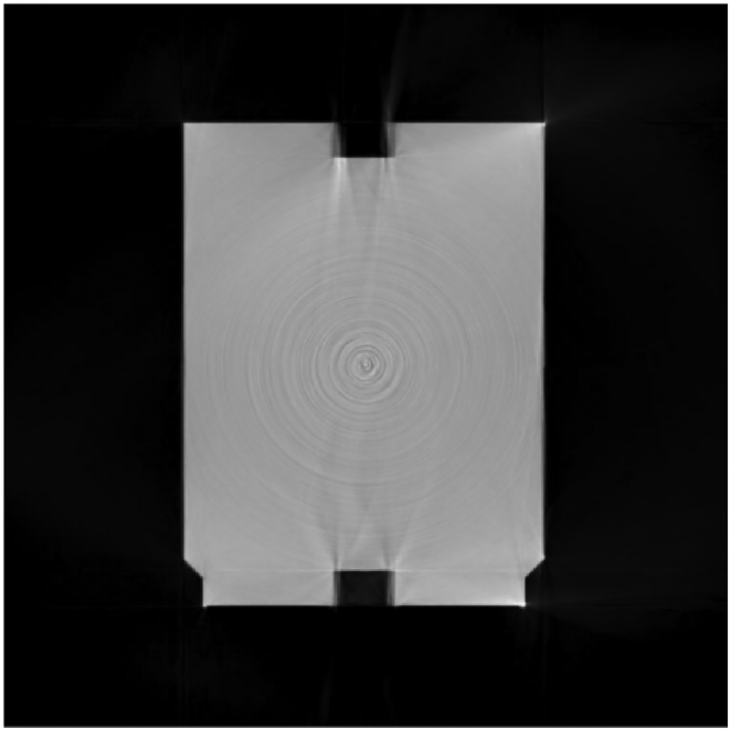
Reconstructed image of an industrial component with added ring artifacts.

Background generation

After model conversion, we obtain reconstructed images with various component contours. However, due to differences in the density distribution of the components, variations in detector response, and electromagnetic noise in the system circuitry, these reconstructed images still exhibit significant differences from actual reconstructed images. Therefore, it is necessary to correct artifacts generated during model conversion and introduce background noise into the images. However, there is no direct correspondence between the simulated reconstructed images obtained from model conversion and the experimental reconstructed images from actual graphite and carbon bricks, making it difficult to naturally merge the two types of images.

To address this issue, we improved upon the CycleGAN¹⁸ model and incorporated data augmentation methods such as random rotation and cropping to manipulate the shape contours and internal textures of the images. We propose the Contour-CycleGAN model, which operates in a semi-supervised manner. In the absence of labeled data, this model is trained by designing two simultaneous tasks and utilizing feedback signals between them to guide the training process. This approach maps simulated images to approximate images with the style and characteristics of actual CT reconstructions, achieving unpaired image style transfer.

Model structure

The overall framework of Contour-CycleGAN is shown in Figure 5. The model includes two generator networks {G, F}, and two discriminator networks {DX, DY}. The generator networks G and F are responsible for mapping images from the simulated CT image style to the actual CT image style, and vice versa. The discriminator networks DX and DY determine whether the generated approximate simulated CT images are sufficiently similar to the simulated CT images, and whether the generated approximate actual CT images are sufficiently similar to the actual CT images, respectively.

Figure 5.

Contour-CycleGAN model framework diagram.

During training, the generator and discriminator networks engage in adversarial learning, where the generators strive to produce increasingly realistic images, and the discriminators continually improve their ability to distinguish generated images from real ones. When the discriminators can no longer effectively differentiate between generated images and real CT images, the generative model is considered to have achieved sufficiently realistic generation.

The four networks collectively form two cyclical processes. The first process, illustrated in the upper part of the diagram, begins by inputting a simulated image X into generator network G, which generates an image G(X) resembling an actual CT image. This generated image is then fed into generator network F, which maps the G(X) image with the actual CT image style back to the simulated CT image style, resulting in F(G(X)), thus completing one cycle. The objective of this cycle is to ensure that the image F(G(X)) closely resembles the original image X, achieving cycle consistency. Therefore, the similarity between the initial image X and F(G(X)) is calculated. The second process works in the reverse order. An actual CT image Y is input into generator network F, producing an image F(Y) with the simulated CT image style. This image is then input into generator network G, resulting in G(F(Y)), which maps back to the actual CT image style. The similarity between the original image Y and G(F(Y)) is then calculated to ensure consistency.

The structure of the generator and discriminator networks is consistent with the original CycleGAN model. As shown in Figure 6, the generator employs an encoder-decoder architecture. The input image first passes through three convolutional layers, which reduce the spatial resolution of the feature maps while increasing the number of channels, thus extracting the original pixel information of the image. The middle part of the generator consists of six consecutive residual convolution blocks. For each residual convolution block, the input feature map passes through both a convolutional branch and a bypass branch. The bypass branch allows shallow information to be rapidly transmitted to deeper layers during forward propagation and accelerates the backward propagation of gradients, preventing the vanishing gradient problem. After all the residual convolution blocks, the feature map undergoes two layers of transposed convolutions and one layer of standard convolution, ultimately producing an output image of the same size as the original input image. The transposed convolutions perform learnable upsampling, yielding superior results compared to traditional methods like bicubic interpolation.

Figure 6.

Schematic diagram of the generator network structure.

The structure of the discriminator network is shown in Figure 7. The output image from the generator is first concatenated with the actual CT image along the channel dimension. The resulting feature map is then input into the discriminator network to assess the similarity between the generator's output image and the actual CT image, thereby determining the realism of the generated image. The discriminator network extracts features and performs downsampling through three convolutional layers with a stride of 2, followed by a standard convolutional layer with a stride of 1 for further feature processing. The final feature map is used to compute the discriminator score, which evaluates the similarity between the generated image and the actual CT image.

Figure 7.

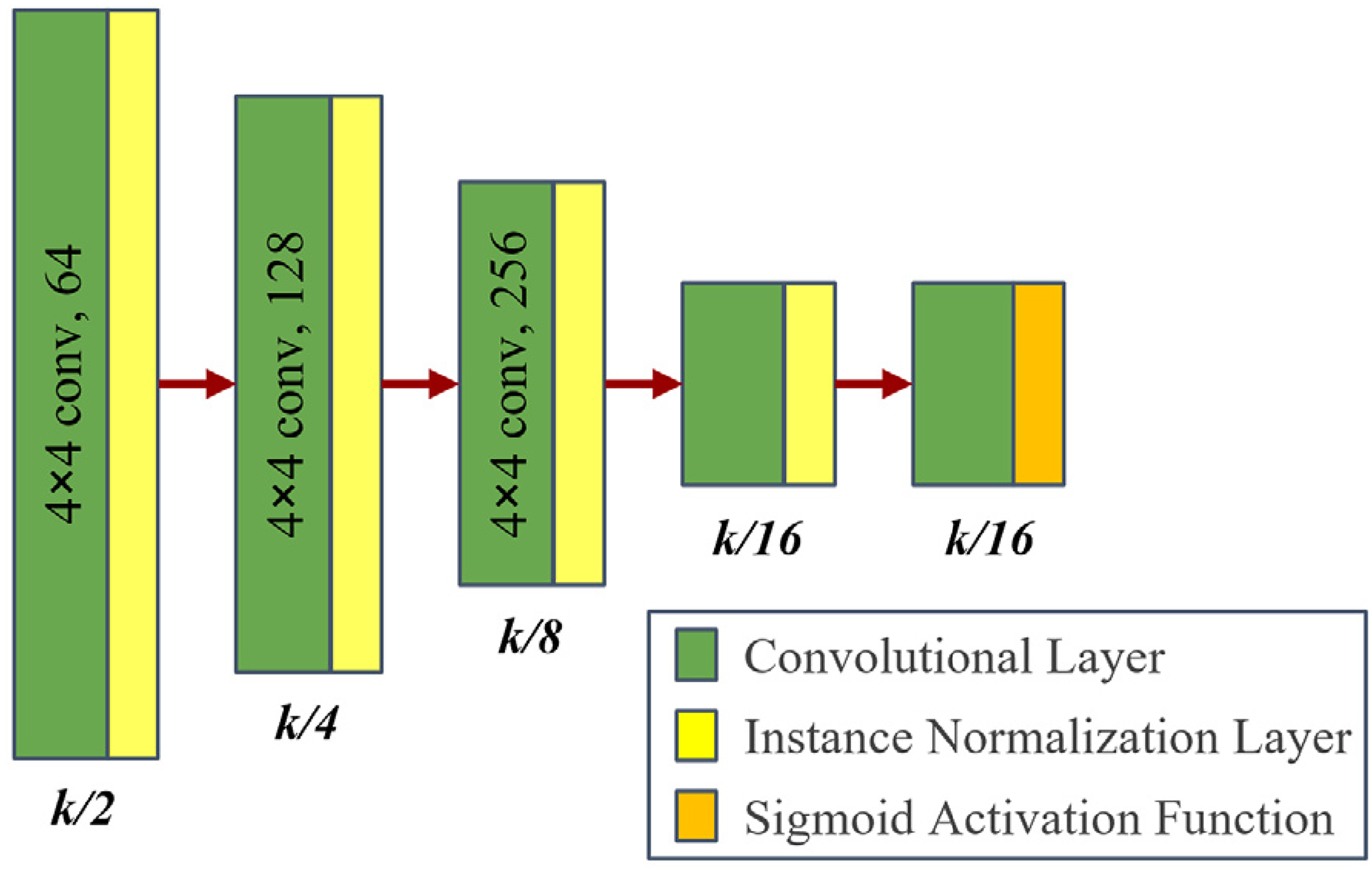
Schematic diagram of the discriminator network structure.

Loss functions

Building upon the CycleGAN design, this paper introduces an additional loss term Loss_cycle–p. The total loss function is formulated as follows:

L o s s = L o s s_{G A N} + L o s s_{c y c l e} + L o s s_{c y c l e - p}

(1)

where:

Adversarial Loss Loss_{G
AN}: This term represents the adversarial loss, encouraging the generator and discriminator to compete and evolve, thus producing realistic images. The formula is:

\begin{aligned} L o s s_{G A N} = L_{G A N} (G, D_{y}, x, y) + L_{G A N} (F, D_{x}, x, y) \\ = E_{y \sim p_{d a t a} (y)} [\log D_{y} (y)] + E_{x \sim p_{d a t a} (x)} [\log (1 - D_{y} (G (x)))] \\ + E_{x \sim p_{d a t a} (x)} [\log D_{x} (x)] + E_{y \sim p_{d a t a} (y)} [\log (1 - D_{x} (F (y)))] \end{aligned}

(2)

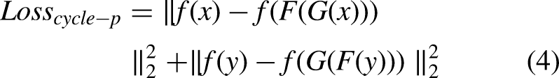
Cycle Consistency Loss Loss_cycle: This term ensures the generated image remains similar to the original after a complete cycle. It uses L1 loss to measure the pixel-wise differences, aiming to preserve the content of the image:

L o s s_{c y c l e} = E_{x \sim p_{d a t a} (x)} [∥ F (G (x)) - x ∥_{1}] + E_{y \sim p_{d a t a} (y)} [∥ G (F (y)) - y ∥_{1}]

(3)

Perceptual Cycle Consistency Loss Loss_cycle–p: For tasks involving background noise generation, L1 loss alone may not achieve high precision due to the inherent uncertainty of noise information. This term uses a neural network f to extract features from the images and computes similarity in the feature domain, aligning more closely with human visual perception:

L o s s_{c y c l e - p} = ∥ f (x) - f (F (G (x))) ∥_{2}^{2} + ∥ f (y) - f (G (F (y))) ∥_{2}^{2}

(4)

In this work, the VGG network is used as the model f, with similarity computed based on feature maps from the 2nd and 5th layers of the network.

Defect synthesis

After completing model conversion and background generation, we obtained simulated images with various shapes and similar textures. To generate defects that closely resemble actual defects, we adopted a method inspired by the Copy-Paste¹⁹ data augmentation technique, utilizing hole defects and loose defects from actual CT images. We propose a method called Copy-Adjust-Paste (CAP) to repeatedly copy and paste actual defects. The key difference between CAP and Copy-Paste is that CAP constrains the placement of defects to the contours of the object, ensuring realism, whereas Copy-Paste does not restrict the placement location, allowing target instances to be pasted anywhere in the image. Additionally, CAP includes grayscale adjustment and edge Gaussian blurring to smooth the transition between defects and the surrounding material.

By incorporating more defects with realistic shapes and numerical characteristics into each simulated image, the CAP method effectively addresses the problems of small sample sizes and class imbalance, thereby improving the accuracy and robustness of defect detection models. Figure 8 illustrates the workflow of this method, with the specific steps outlined below:

Annotate and compile defects from existing experimental CT reconstructed images to create a defect library.

For each simulated image to be generated, after model conversion and background generation, randomly sample several defects from the defect library and sequentially read the sampled defect information.

Randomly translate and rotate the defect instances, and perform image dilation.

Check whether the newly dilated defects exceed the contour boundaries or overlap with existing defects. If they do, repeat step 3.

Adjust the grayscale values of the new defects to match the current image.

Apply Gaussian blurring to the edges of the new defects to ensure a natural transition with the surrounding image.

Figure 8.

Workflow diagram of the CAP method for defect synthesis.

In the workflow described above, Step 3 involves randomly translating and rotating defects to increase the diversity of their positions and orientations, thereby enhancing the model's ability to capture different defect shapes. Additionally, because grayscale values can vary between different reconstructed images or even within different regions of the same image, directly copying defects onto new images may result in unnatural boundaries. To address this, Step 3 includes image dilation of the translated and rotated defects, which facilitates the adjustment of grayscale values in subsequent steps. In Step 5, grayscale values are adjusted by calculating the average grayscale value of the defect's surrounding area in the original image and then matching the new defect and its neighboring region to this average value. This ensures that the relative grayscale variation between the defect and its neighboring area remains consistent with the original image. Following this, Step 6 applies Gaussian blurring to the edges of the new defects, ensuring a smooth transition between the defects and the base material. This process results in a more natural integration of the defects into the new image.

Experiment and results

All experiments were conducted on a computer equipped with an Intel i7-12700 CPU, 32 GB of RAM, and an NVIDIA GeForce RTX 3080 GPU, using Python and the PyTorch deep learning framework.

Contour-CycleGAN

Dataset

To generate the dataset, we followed the model conversion method to create a dataset of 2000 images in the simulated CT image style and selected 2000 images in the actual CT image style for model training.

In the existing dataset, all training samples have fixed orientations. For instance, all simulated images are oriented vertically (Figure 9(a)), and all actual reconstructed images have the same rotation angle (Figure 9(b)). Training the model directly on these data would introduce inherent biases, leading the model to mistakenly learn the rotation angle as a target feature, resulting in generated images with fixed rotation angles. Therefore, during training, we randomly rotate the input images in each batch to eliminate this phase-specific fixed orientation.

Figure 9.

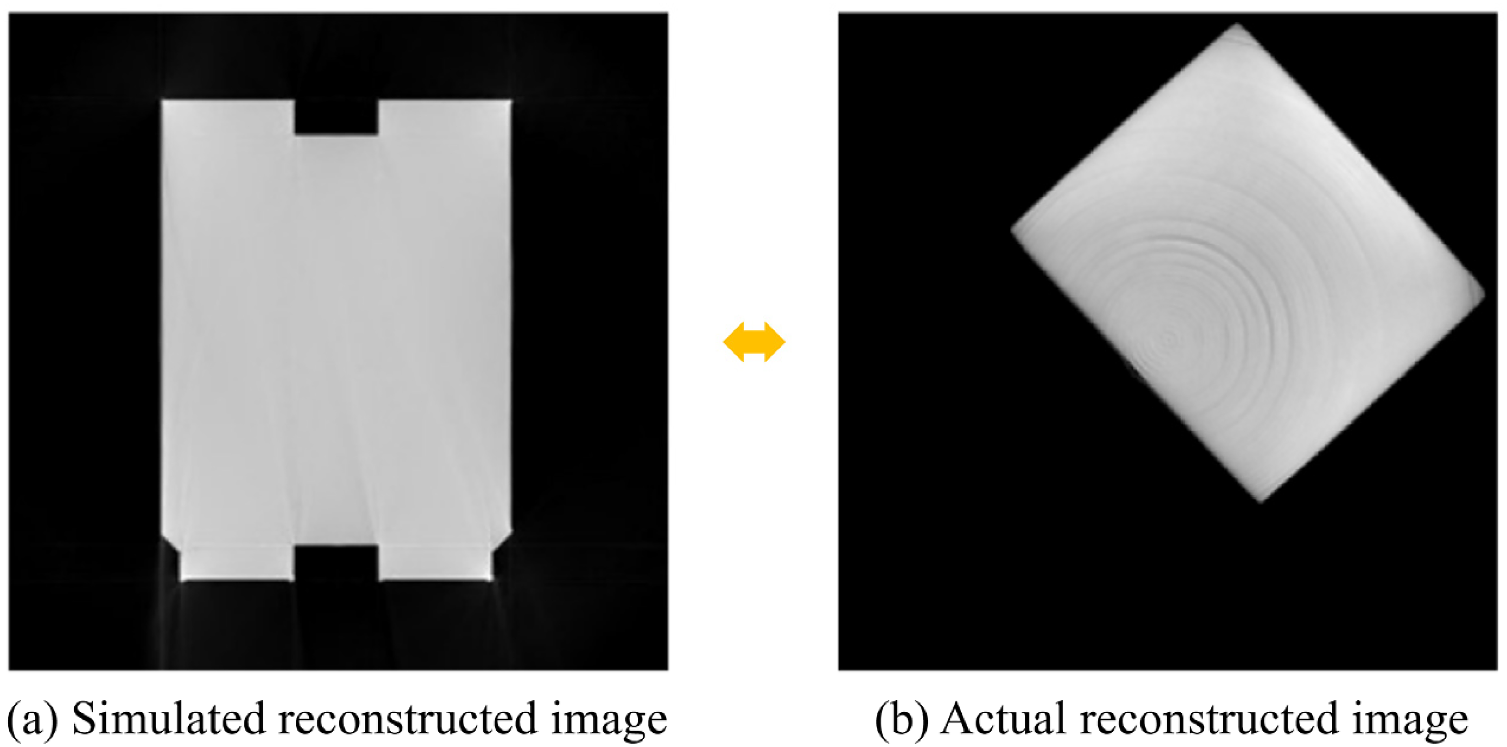
Comparison between simulated reconstructed images and actual reconstructed images.

Additionally, given that actual CT reconstructed images often have uniform dimensions, we proposed a random cropping data augmentation method. Specifically, after each random rotation, we crop the image contours or internal textures at a predetermined probability to eliminate size uniformity, allowing the model to focus on learning the representation of texture structures and background noise (as shown in Figure 10).

Figure 10.

Illustration of the random cropping data augmentation effect.

Training details

During training, we adhered to the same settings as those used in CycleGAN. Each training batch contained a single sample input to the neural network, and we utilized the Adam optimizer²⁰ for model training. The initial learning rate was set to 2 × 10⁻⁴ and maintained for the first 100 epochs, followed by a linear decay over the next 100 epochs. Compared to the original CycleGAN model, Contour-CycleGAN incorporates an additional perceptual cycle consistency loss Loss_cycle–p and employs data augmentation techniques such as random rotation and cropping. The perceptual cycle consistency loss encourages the model to learn deeper features of the images, reducing the impact of noise information on feature learning. The data augmentation techniques—random rotation and cropping, help the model learn the texture and contour features of the base material, preventing the inherent bias from fixed orientations and shapes from affecting the training process.

Training results

The images generated by the Contour-CycleGAN model are shown in Figure 11. It is evident that Contour-CycleGAN preserves the shape and contour information of the images while focusing on processing the internal textures. The processed images visually resemble actual CT images, particularly in terms of ring artifacts and background noise. Compared to the output images from model conversion, the ring artifacts in the generated images appear more realistic, and a certain degree of background noise is introduced. Furthermore, the grayscale distribution of the generated images closely matches that of actual CT images, exhibiting similar variations in light and dark regions. This results in processed images with uniform grayscale distributions, aside from the introduced ring artifacts, aligning well with the characteristics of actual CT images.

Figure 11.

Background generation effects of the contour-CycleGAN model.

To achieve a more comprehensive assessment of imaging performance, this study employs the Learned Perceptual Image Patch Similarity (LPIPS) metric,²¹ which more accurately reflects human visual perception compared to traditional metrics. The LPIPS metric evaluates the perceptual distance between image patches by leveraging features extracted by deep neural networks (AlexNet used in this study). Images x and x₀ are input into the AlexNet network where features ${\hat{y}}^{l}$ and ${\hat{y}}_{0}^{l}$ are extracted at each convolutional layer l, subsequently normalized, and a weighting vector $w_{l}$ is applied to these normalized features. The weighted Euclidean distances are calculated at each layer, with the overall LPIPS score derived by summing these distances across all layers:

d (x, x_{0}) = \sum_{l} \frac{1}{H_{l} W_{l}} \sum_{h, w} w_{l} ⊙ {({\hat{y}}_{h w}^{l} - {\hat{y}}_{0 h w}^{l})}_{2}^{2}

(5)

Where $H_{l}$ , $W_{l}$ , and $C_{l}$ represent the height, width, and number of channels of the feature map at each layer, respectively. A lower LPIPS value indicates greater perceptual similarity between the two images.

In our experimental evaluation, we utilized LPIPS version 0.1 to ensure the consistency and reliability of our results. The LPIPS score obtained was 0.1786, indicating a high degree of perceptual similarity between the generated and actual CT images. This low score substantiates the superior performance of the Contour-CycleGAN in producing images that are not only technically accurate but also visually comparable to real CT scans.

Discussion

To evaluate the impact of key operations in the image generation process on the final results, we conducted a set of comparative experiments. Specifically, we removed the ring artifact generation step in the model conversion process and trained the model using the original CycleGAN, keeping all other training details identical. The experimental results are shown in Figure 12.

Figure 12.

Test results of the CycleGAN model.

It can be observed that after training the model with CycleGAN on images without ring artifacts, the output images exhibited some internal textures, but these textures lacked the distinctive ring patterns and instead displayed non-ring, scaly structures, which do not match the characteristics of actual CT images. This discrepancy arises because the internal textures of simulated images differ significantly from those of actual images, and without additional information, CycleGAN struggles to learn the mapping of these differences effectively, capturing only partial texture features. In contrast, when trained on data containing weak ring artifacts, both simulated and actual images possess ring artifact textures, differing only in degree and distribution, which makes it easier for the model to learn the mapping between them.

Additionally, observing the image contours reveals that the output images generated by the CycleGAN model tend to reduce the size of the objects compared to the input images. This limitation hinders the model's ability to generate images with diverse shapes. In contrast, the Contour-CycleGAN model, which incorporates random rotation and cropping operations, maintains the consistency of the input image sizes, as shown in Figure 11. This consistency is achieved because the simulated data in the training dataset generally have larger object sizes compared to the actual data. When training directly with CycleGAN, the model learns object size as a feature, which affects the final generation results. However, the random rotation and cropping operations in Contour-CycleGAN alter the image contours and sizes, eliminating the inherent bias in contour size between the simulated and actual data. This adjustment prevents the model from learning object size as a distinguishing feature during training, thereby ensuring that the output images maintain consistent sizes.

Copy-Adjust-Paste (CAP)

Implementation details

For the images obtained after model conversion and background generation, we applied the CAP method for defect synthesis. The defect images were dilated by 10 pixels, and Gaussian blur with a variance of σ = 1 was applied to the edges. Each generated image included 10 hole defects and 4 loose defects. Compared to hole defects, loose defects are larger, more heterogeneous areas with smaller grayscale differences. In the existing experimental data, loose defect samples are sparse and unevenly distributed, potentially affecting the model's ability to detect such defects. By using the CAP method, these loose defects can appear at any location within the image, thus decoupling defects from specific positions and addressing the problem of imbalanced defect samples.

Experimental results

The CAP synthesis results for hole and loose defects are shown in Figure 13. The simulated image defects generated by CAP exhibit similar data distribution characteristics to those in the experimental images. These defects blend naturally into the images without noticeable artificial transitions at the edges, maintaining consistent grayscale variation with the surrounding areas. By comparing the red boxes in Figure 13, it is evident that the hole and loose defects in the generated CT images closely resemble the defect patterns in real CT images, with highly similar detail characteristics. This highlights the effectiveness of the CAP method in expanding the defect sample set. By sourcing actual defects and embedding them into various base backgrounds, CAP significantly enriches the training sample set for defect detection models.

Figure 13.

Illustration of CAP synthesis effects for hole and loose defects.

Discussion

Figure 14 illustrates the defect synthesis effects using different methods on simulated images. In Figure 14(a), the defects introduced using the Copy-Paste method exhibit obvious unnatural boundaries. This issue arises because the grayscale distribution within the reconstructed images is not uniform. If a defect from a high grayscale value region is directly copied to a low grayscale value region, the defect's grayscale value may be higher than that of the surrounding area. Consequently, the Copy-Paste method fails to maintain consistent grayscale variations between the defect and its surrounding region. In contrast, in Figure 14(b), the CAP method adjusts the grayscale values of the defects based on those of the surrounding area, preserving the relative grayscale changes. Combined with edge Gaussian blurring, this results in a more natural transition between the defects and their surroundings, providing better visual integration.

Figure 14.

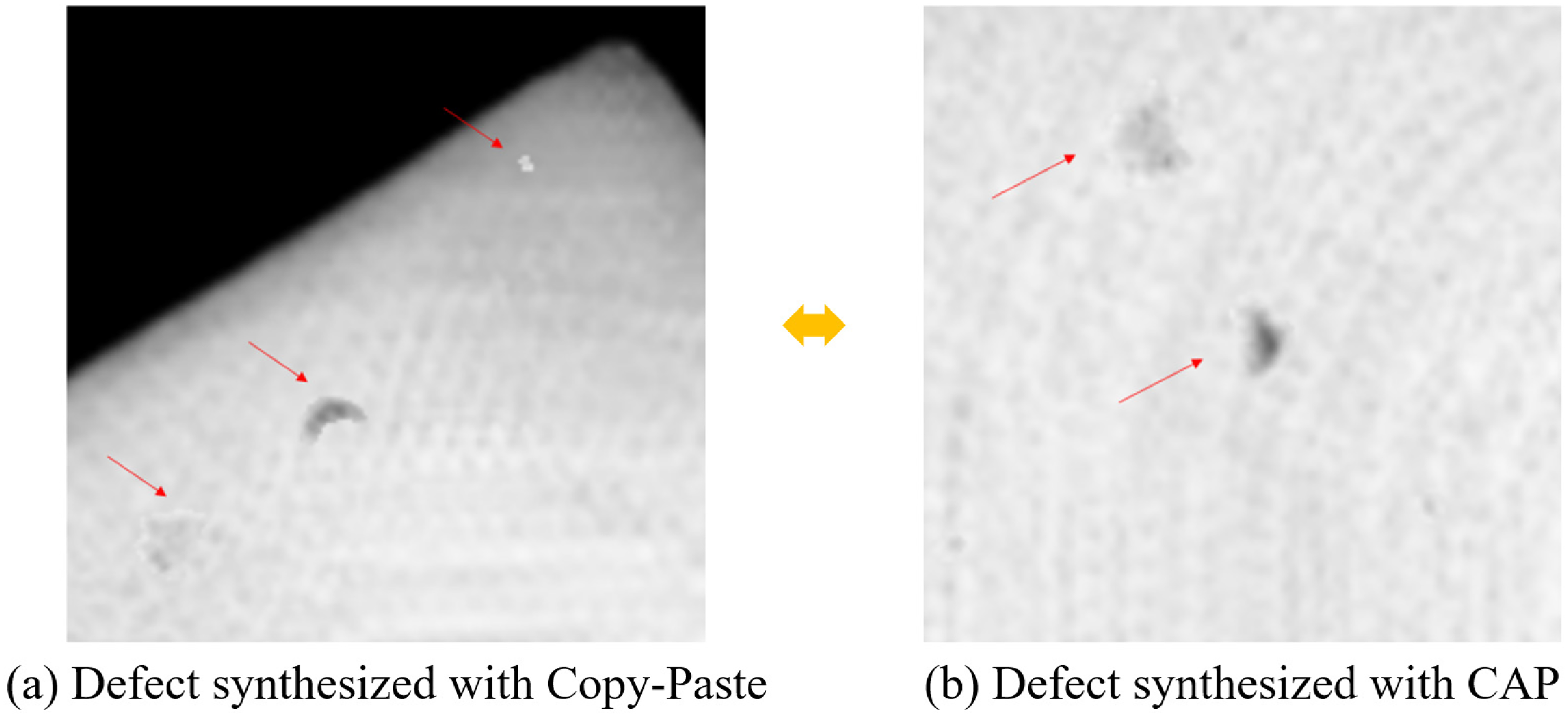
Comparison of defect synthesis effects using copy-paste and CAP methods.

Discussion

The primary objective of the proposed Decompound Synthesize Method (DSM) is to address the problems of small sample sizes and class imbalance in defect detection model training, thereby improving the accuracy of defect detection models. Therefore, beyond visually assessing the similarity between the generated images and actual images, it is essential to experimentally validate the effectiveness of the DSM in enhancing defect detection.

Experimental setup

This experiment aims to validate the effectiveness of the DSM method in training defect detection models. We used the existing object detection network model Mask R-CNN²² and compared its performance on different datasets. The basic structure of Mask R-CNN is shown in Figure 15. The model first processes the input image through a convolutional neural network for feature extraction. Then, the Region Proposal Network (RPN)²³ outputs several Regions of Interest (RoIs) that are likely to contain targets. Finally, a classifier and regressor are used to determine the target's category and coordinates, while a parallel branch generates pixel-level binary instance segmentation masks for each RoI.

Figure 15.

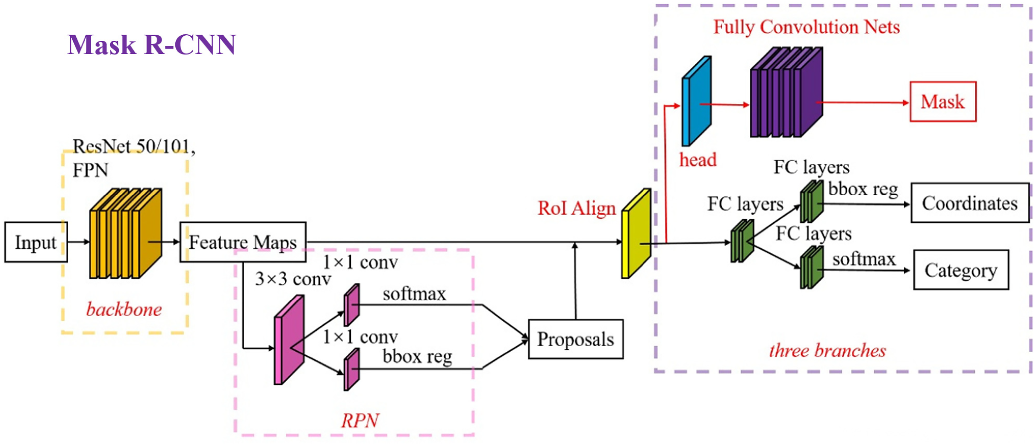
Structure of the mask R-CNN model.

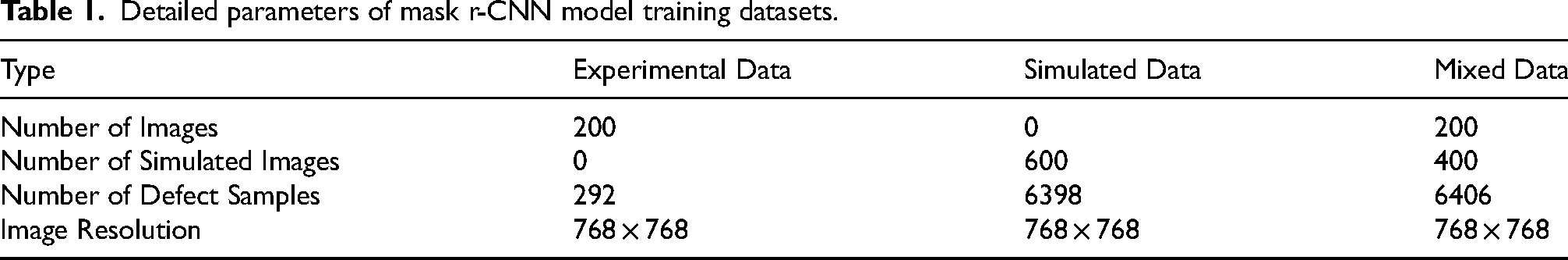
Regarding the dataset, we prepared three groups of datasets with identical validation sets but different training sets. The first group consisted of 200 original CT reconstructed images with defects. The second group contained 600 images generated entirely using the DSM. The third group comprised a mix of 200 original CT reconstructed images and 400 DSM-generated images, totaling 600 images. Additionally, the validation set consisted of 20 experimental CT reconstructed images that were not included in the training sets. The detailed composition of the three datasets is shown in Table 1. The resolution of all images is 768 × 768 pixels, and defects are categorized into holes, side defects, and looseness.

Table 1.

Detailed parameters of mask r-CNN model training datasets.

Type	Experimental Data	Simulated Data	Mixed Data
Number of Images	200	0	200
Number of Simulated Images	0	600	400
Number of Defect Samples	292	6398	6406
Image Resolution	768 × 768	768 × 768	768 × 768

For training details, we used the open-source object detection tool MMDetection,²⁴ maintaining the original settings of Mask R-CNN. The SGD optimizer was used, with ResNet50 as the pre-trained weights. The initial learning rate was set to 0.02, with a weight decay coefficient of 0.0001, and the learning rate was reduced to 0.001 at the 8th and 11th epochs, for a total of 12 epochs. All network hyperparameters were kept consistent with the original paper.

Result analysis

In this experiment, we used Mean Average Precision (mAP),²⁵ a common evaluation metric in the field of object detection, to measure the accuracy of the defect detection model. Table 2 presents the training results using different datasets. It can be observed that when the model was trained solely on experimental data, the mAP was only 0.342. Training on simulated data improved the mAP to 0.456. The highest mAP of 0.589 was achieved when the model was trained on the mixed dataset.

Table 2.

Training results using different datasets.

Data Type	Experimental Data	Simulated Data	Mixed Data
mAP	0.342	0.456	0.589

However, it should be noted that although training with the mixed dataset achieved the highest detection accuracy so far, the precision is still not high enough for defect detection tasks. Figure 16 shows a CT reconstructed image with defect labels and the detection results of the model trained on the mixed dataset. The image contains five actual defects, but the model only detects two of them and the confidence scores for the hole defects is only 0.40. Therefore, while training on the mixed dataset improves the average precision compared to using only experimental or simulated data, further research on the model architecture and evaluation metrics is needed to enhance the performance of the defect detection model to make it fully applicable to this task.

Figure 16.

Comparison of defect detection results using the mask R-CNN model with the mixed dataset.

Conclusions

This study introduces the Decompound Synthesize Method (DSM), a novel algorithm for CT detection image generation designed to mitigate the challenges of small sample sizes and class imbalance in defect detection. The DSM algorithm strategically divides the image generation process into three steps: model conversion, background generation, and defect synthesis. Each step employs adaptive methods to produce synthetic samples that closely mirror actual CT images, thereby enriching the training dataset and enhancing model training effectiveness. Our experimental findings affirm DSM's capability to significantly improve the performance of defect detection models, as demonstrated by increased mean Average Precision (mAP) metric when utilizing DSM-generated and mixed datasets.

Despite these advancements, the experiments have also highlighted some limitations of the DSM approach in defect detection applications. While detection accuracy has notably improved, ongoing refinement and optimization of the algorithm are essential. Future research should focus on developing more sophisticated methods for model conversion, background generation, and defect synthesis to elevate the quality and authenticity of generated images. Enhancing the DSM algorithm's structure and training protocols, integrating more authentic data, and exploring additional strategies to overcome the challenges of small sample sizes and class imbalance are imperative. Moreover, refining the evaluation metrics and the architectural design of defect detection models will be crucial in advancing the field. By addressing these aspects, the reliability and accuracy of defect detection tasks can be significantly improved, leading to more effective industrial applications.

Footnotes

ORCID iDs

Jintao Fu

Tianchen Zeng

Ximing Liu

Funding

The authors received no financial support for the research, authorship, and/or publication of this article.

Declaration of conflicting interests

The authors declared no potential conflicts of interest with respect to the research, authorship, and/or publication of this article.

References

Liu

Sun

Liu

, et al. Defect detection in the graphite components and carbon bricks in high temperature gas-cooled reactors using helical CT. Journal of Tsinghua University(Science and Technology) 2021; 61: 367–376. [in Chinese].

Kunerth

McJunkin

. Nondestructive evaluation of nuclear-grade graphite. AIP Conference Proceedings 2012; 1430: 1609–1616.

Khanam

Hussain

Hill

, et al. A comprehensive review of convolutional neural networks for defect detection in industrial applications. IEEE Access 2024; 12: 94250–94295.

Palma-Ramírez

, et al. Deep convolutional neural network for weld defect classification in radiographic images. Heliyon 2024; 10.

Wang

Gao

Song

. Applying SDR with CNN to identify weld defect: a new processing method. Journal of Pipeline Systems Engineering and Practice 2023; 14: 06023001.

Goceri

. Medical image data augmentation: techniques, comparisons and interpretations. Artif Intell Rev 2023; 56: 12561–12605.

Martins

DHCSS

, et al. Hybrid data augmentation method for combined failure recognition in rotating machines. J Intell Manuf 2023; 34: 1795–1813.

Shorten

Khoshgoftaar

. A survey on image data augmentation for deep learning. J Big Data 2019; 6: 60.

Perez

Wang

. The effectiveness of data augmentation in image classification using deep learning. Convolutional Neural Networks Vis. Recognit 2017; 11: 1–8.

10.

Randellini

Rigutini

Sacca

. Data augmentation and transfer learning approaches applied to facial expressions recognition. International Journal of Artificial Intelligence and Applications 2022; 13: 55–72.

11.

Few-shot classification via efficient meta-learning with hybrid optimization. Engineering Applications of Artificial Intelligence 2024; 127: 107296.

12.

Xie

Long

, et al. Joint distribution matters: deep Brownian distance covariance for few-shot classification. In: 2022 IEEE/CVF conference on computer vision and pattern recognition (CVPR). 2022, pp.7962–7971.

13.

Lin

T-Y

Goyal

Girshick

, et al. Focal loss for dense object detection. In: 2017 IEEE international conference on computer vision (ICCV). 2017, pp.2999–3007.

14.

Khan

Chaudhari

Chandra

. A review of ensemble learning and data augmentation models for class imbalanced problems: combination, implementation and evaluation. Expert Systems with Applications 2024; 244: 122778.

15.

Ding

Huang

, et al. LEGAN: addressing intraclass imbalance in GAN-based medical image augmentation for improved imbalanced data classification. IEEE Transactions on Instrumentation and Measurement 2024; 73: 1–14.

16.

Goodfellow

Pouget-Abadie

Mirza

, et al. Generative adversarial nets. Communications of the ACM 2020; 63: 139–144.

17.

Tran

Yan

Fang

. Improving model-based fNIRS analysis using mesh-based anatomical and light-transport models. Neurophotonics 2020; 7: 015008.

18.

Zhu

J-Y

Park

Isola

, et al. Unpaired image-to-image translation using cycle-consistent adversarial networks. In: 2017 IEEE international conference on computer vision (ICCV). 2017, pp.2242–2251.

19.

Ghiasi

, et al. Simple copy-paste is a strong data augmentation method for instance segmentation. In: 2021 IEEE/CVF conference on computer vision and pattern recognition (CVPR). 2021, pp.2917–2927.

20.

Kingma

. Adam: a method for stochastic optimization. AIP Conf Proc 2017; 1631: 58–62.

21.

Zhang

Isola

Efros

, et al. The unreasonable effectiveness of deep features as a perceptual metric. In: 2018 IEEE/CVF conference on computer vision and pattern recognition. 2018, pp.586–595.

22.

Gkioxari

Dollár

, et al. Mask R-CNN. In: 2017 IEEE international conference on computer vision (ICCV). 2017, pp.2980–2988.

23.

Ren

Girshick

, et al. Faster R-CNN: towards real-time object detection with region proposal networks. IEEE Transactions on Pattern Analysis and Machine Intelligence 2017; 39: 1137–1149.

24.

Chen

, et al. “MMDetection: Open MMLab Detection Toolbox and Benchmark,” Jun. 17, 2019, arXiv: arXiv:1906.07155. DOI: 10.48550/arXiv.1906.07155.

25.

Zhao

Z-Q

Zheng

S-T

, et al. Object detection with deep learning: a review. IEEE Transactions on Neural Networks and Learning Systems 2019; 30: 3212–3232.