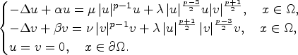
Infinitely Many Sign-Changing Solutions for Coupled Schrödinger System

Abstract

In this article, we study the following coupled Schr $\ddot{o}$ dinger system with subcritical exponent: ${\begin{cases} - Δ u + α u = μ | u |^{p - 1} u + λ | u |^{\frac{p - 3}{2}} u | v |^{\frac{p + 1}{2}}, x \in Ω, \\ - Δ v + β v = ν | v |^{p - 1} v + λ | u |^{\frac{p + 1}{2}} | v |^{\frac{p - 3}{2}} v, x \in Ω, \\ u = v = 0, x \in \partial Ω . \end{cases}$ Here, either $Ω = R^{N}$ or $Ω$ is a smooth bounded domain in $R^{N}$ with $N \geq 4$ ; positive constants $α, β, μ, ν > 0$ and the coupling constant $λ < 0$ , $1 < p < 2^{*} - 1$ , $2^{*} = 2 N / N - 2$ is the critical Sobolev exponent. We show that, this system has infinitely many radially symmetric sign-changing solutions and infinitely many radially symmetric semi-nodal solutions. Moreover, we obtain a least energy sign-changing solution for $α > - λ_{1} (Ω), β > - λ_{1} (Ω)$ in the following sense: one component is positive and the other one changes sign which has exactly two nodal domains.

Keywords

Sign-changing solutions Schrödinger system nodal domains

1. Background and Main Results

Consider the following nonlinear coupled Schr $\ddot{o}$ dinger system:

{\begin{cases} - Δ u + α u = μ | u |^{p - 1} u + λ | u |^{\frac{p - 3}{2}} u | v |^{\frac{p + 1}{2}}, x \in Ω, \\ - Δ v + β v = ν | v |^{p - 1} v + λ | u |^{\frac{p + 1}{2}} | v |^{\frac{p - 3}{2}} v, x \in Ω, \\ u = v = 0, x \in \partial Ω . \end{cases}

(1.1)

Here, either

Ω = R^{N}

Ω

is a smooth bounded domain in

R^{N} (N \geq 4)

α, β, μ, ν

are positive parameters and

λ \neq 0

is a coupling constant.

In the case $N = 2, 3$ and $p = 3$ , system (1.1) becomes the cubic system:

{\begin{cases} - Δ u_{1} + α u_{1} = μ u_{1}^{3} + λ u_{1} u_{2}^{2}, x \in Ω, \\ - Δ u_{2} + β u_{2} = ν u_{2}^{3} + λ u_{1}^{2} u_{2}, x \in Ω, \\ u_{1} = u_{2} = 0 on \partial Ω, \end{cases}

(1.2)

which arises in the study of many physical phenomena like nonlinear optics and Bose-Einstein condensation (cf. Frantzeskakis, 2010; Kivshar & Luther-Davies, 1998). Therefore, in the last decades, the system (1.2) has received great interest from mathematicians. When

Ω

is the entire space

R^{N}

, the existence of least energy and other finite energy solutions of (1.2) was studied by Ambrosetti and Colorado (2007), Bartsch and Wang (2006), Bartsch et al. (2007), Chen and Zou (2012), Lin and Wei (2005a), Liu and Wang (2008), Liu and Wang (2010), Maia et al. (2006), Maia et al. (2008), Sirakov (2007), and Terracini and Verzini (2009) and references therein. In particular, when

λ > 0

is sufficiently large, infinitely many radially symmetric sign-changing solutions of (1.2) were obtained by Maia et al. (2008). Liu and Wang (2010) studied a general

m

-coupled system (

m \geq 2

) and proved that system (1.2) has infinitely many nontrivial solutions, but whether solutions obtained by Liu and Wang (2010) are positive or sign-changing can not be determined there (see also Liu & Wang, 2008). A similar problem is considered in dimension

N = 1

and solutions with exactly

(k_{1}, k_{2})

nodal regions are obtained, for every

(k_{1}, k_{2})

by Terracini and Verzini (2002). When

Ω \subset R^{N} (N = 2, 3)

is a smooth bounded domain, there are also many papers studying (1.2). Lin and Wei (2005b) proved that a least energy solution of (1.2) exists within an appropriate range of

λ

. Dancer et al. (2010a) and Noris and Ramos (2010) proved the existence of infinitely many positive solutions of (1.2). When

Ω

is a ball, a multiplicity result on positive radially symmetric solutions was given by Wei and Weth (2008b). Later, by using a global bifurcation approach, the result of Wei and Weth (2008b) was reproved by Bartsch et al. (2010) without requiring the symmetric condition. Under some more general assumptions, Sato and Wang (to appear) proved that system (1.2) has infinitely many semi-positive solutions (i.e., at least one component is positive). According to Dancer et al. (2010b), the authors proved the existence of unbounded sequence solutions for

N \leq 3

and

λ \leq - 1

. As pointed out above, for

λ \leq - 1

, Wei and Weth (2008a) proved that (1.2) has a radially symmetric solution which turns out to be a positive solution.

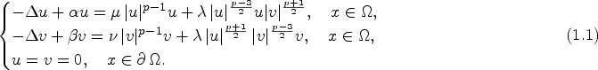
We remark that, the existence of infinitely many sign-changing solutions or semi-nodal solutions to (1.2) was solved by Chen et al. (2016) and Liu et al. (2015) independently, where $N \leq 3, λ < 0.$

To the best of our knowledge, the existence of infinitely many sign-changing solutions, infinitely many semi-nodal solutions and least energy sign-changing solutions to (1.1) has not ever been studied in the literature when $Ω \subset R^{N}$ or $Ω = R^{N}$ , $N \geq 4$ and $1 < p < 2^{*} - 1$ . The main goal of the current article is to solve this problem (1.1) when $λ < 0$ .

Definition 1.1

A solution $(u, v)$ is called nontrivial if $u ≢ 0$ and $v ≢ 0$ , called semi-trivial if $(u, v)$ is the type of $(u, 0)$ or $(0, v)$ . We call a solution $(u, v)$ positive if $u > 0, v > 0$ in $R^{N}$ , a solution $(u, v)$ sign-changing if both $u$ and $v$ change sign, a solution $(u, v)$ semi-nodal if one component changes sign and the other one is positive.

Theorem 1.1

Let $Ω = R^{N}$ , $N \geq 4$ , $α, β, μ, ν > 0$ , and $λ < 0$ . Then system (1.1) has infinitely many radially symmetric sign-changing solutions.

We also study some further properties of the sign-changing solutions obtained in Theorem 1.1. We call a sign-changing solution a least energy sign-changing solution if it has the least energy among all sign-changing solutions. Precisely, we have the following theorem.

Theorem 1.2

Let $Ω = R^{N}$ , $N \geq 4$ , $α, β, μ, ν > 0$ , and $λ < 0$ . Then system (1.1) has a least energy radially symmetric sign-changing solution $(u_{0}, v_{0})$ among all radially symmetric sign-changing solutions such that both $u_{0}$ and $v_{0}$ have exactly two nodal domains.

Both Theorems 1.1 and 1.2 are concerned with sign-changing solutions. Besides positive solutions (obtained by Wei & Weth, 2008a) and sign-changing solutions, we can prove that (1.1) has semi-nodal solutions as defined in Definition 1.1.

Theorem 1.3

Let $Ω = R^{N}$ , $N \geq 4$ , $α, β, μ, ν > 0$ , and $λ < 0$ . Then system (1.1) has infinitely many radially symmetric semi-nodal solution ${(u_{n}, v_{n})}_{n \geq 2}$ such that (1)

$u_{n}$ is positive and $v_{n}$ changes sign;

(2)

$v_{n}$ has at most $n$ nodal domains.

Finally, we consider the case of the smooth bounded domain $Ω \subset R^{N}$ .

Theorem 1.4

Let $Ω \subset R^{N}$ be a smooth bounded domain, $N \geq 4$ , $α > - λ_{1} (Ω), β > - λ_{1} (Ω), μ > 0, ν > 0$ and $λ < 0$ . Then system (1.1) has infinitely many sign-changing solutions ${(u_{n}, v_{n})}_{n \geq 1}$ such that

‖ u_{n} ‖_{L^{\infty} (Ω)} + ‖ v_{n} ‖_{L^{\infty} (Ω)} \to + \infty, as n \to \infty .

Moreover, system (1.1) has a least energy sign-changing solution

(u_{0}, v_{0})

such that both

u_{0}

and

v_{0}

have exactly two nodal domains, where

λ_{1} (Ω)

is the first Dirichlet eigenvalue of

Ω

Theorem 1.5

Let $Ω \subset R^{N}$ be a smooth bounded domain, $N \geq 4$ , $α > - λ_{1} (Ω), β > - λ_{1} (Ω), μ > 0, ν > 0$ . Then system (1.1) has infinitely many semi-nodal solutions ${(u_{n}, v_{n})}_{n \geq 2}$ such that (1)

$u_{n}$ is positive and $v_{n}$ changes sign;

(2)

$v_{n}$ has at most $n$ nodal domains.

The structure of this article is as follows. In Section 2, we prove the existence of infinitely many sign-changing solutions. The main tool will be the new vector genus introduced by Tavares and Terracini (2012) and the constrained problem introduced by Chen et al. (2016), we will construct new minimax values. Remark that the ideas by Chen et al. (2016) and Tavares and Terracini (2012) cannot be used directly, and we will give some new ideas. The crucial idea in this article is turning to study a new problem with two constraints in order to obtain sign-changing solutions of (1.1). This idea has never been used for (1.1) in the literature up to our knowledge. Section 3 is then dedicated to the proof of Theorem 1.2 by using a minimizing argument. In Section 4, we will present the proof of Theorem 1.3 by applying the arguments in Sections 2 and 3. Finally, in the last section, we will consider the case of $Ω \subset R^{N}$ .

We give some notations here. Throughout this article, we denote the norm of $L^{p} (R^{N})$ by $| u |_{p} = (\int_{R^{N}} | u |^{p} d x)^{\frac{1}{p}}$ , the norm of $H^{1} (R^{N})$ by $‖ u ‖^{2} = \int_{R^{N}} (| \nabla u |^{2} + | u |^{2}) d x$ and the positive constants (possibly different in different places) by $C$ . Define the radial space $H_{r} := H_{r}^{1} (R^{N}) \times H_{r}^{1} (R^{N})$ as a subspace of $H := H^{1} (R^{N}) \times H^{1} (R^{N})$ with norm $‖ (u, v) ‖_{H_{r}}^{2} := ‖ u ‖_{α}^{2} + ‖ v ‖_{β}^{2}$ where $‖ u ‖_{α}^{2} := \int_{R^{N}} (| \nabla u |^{2} + α | u |^{2}) d x$ and

H_{r}^{1} (R^{N}) := {u \in H^{1} (R^{N}) : u is radially symmetric} .

2. Proof of Theorem 1.1

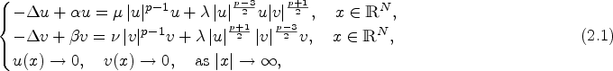
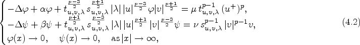
In this section, we consider the case $Ω = R^{N}$ . That is, we consider the following elliptic system in the entire space:

{\begin{cases} - Δ u + α u = μ | u |^{p - 1} u + λ | u |^{\frac{p - 3}{2}} u | v |^{\frac{p + 1}{2}}, x \in R^{N}, \\ - Δ v + β v = ν | v |^{p - 1} v + λ | u |^{\frac{p + 1}{2}} | v |^{\frac{p - 3}{2}} v, x \in R^{N}, \\ u (x) \to 0, v (x) \to 0, as | x | \to \infty, \end{cases}

(2.1)

where

N \geq 4

1 < p < 2^{*} - 1

α, β, μ, ν > 0

, and

λ < 0

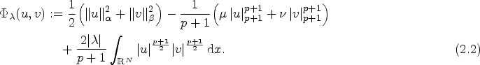
. It is well-known that the radial solutions of (2.1) are the critical points of the

C^{2}

functional

Φ_{λ} : H_{r} \to R

given by the following equation:

\begin{aligned} Φ_{λ} (u, v) & := \frac{1}{2} (‖ u ‖_{α}^{2} + ‖ v ‖_{β}^{2}) - \frac{1}{p + 1} (μ | u |_{p + 1}^{p + 1} + ν | v |_{p + 1}^{p + 1}) \\ + \frac{2 | λ |}{p + 1} \int_{R^{N}} | u |^{\frac{p + 1}{2}} | v |^{\frac{p + 1}{2}} d x . \end{aligned}

(2.2)

We will look for solutions of equation (2.1) as critical points of the functional

Φ_{λ}

restricted to the sphere

A := {(u, v) \in H_{r} : | u |_{p + 1} = 1, | v |_{p + 1} = 1} .

(2.3)

In order to obtain infinitely many radially symmetric sign-changing critical points, we need to define several minimax energy levels using a new definition of vector genus introduced by Tavares and Terracini (2012). According to Tavares and Terracini (2012), we take the transformations

σ_{i} : A \to A, σ_{1} (u, v) = (- u, v), σ_{2} (u, v) = (u, - v), i = 1, 2.

Consider the class of sets

F = {A \subset A : A \,is a closed set and σ_{i} (u, v) \in A, \forall (u, v) \in A, i = 1, 2}

and for each

A \in F

and

k_{1}, k_{2} \in N

, the class of functions

\begin{aligned} F_{(k_{1}, k_{2})} (A) & = {f = (f_{1}, f_{2}) : A \to \prod_{i = 1}^{2} R^{k_{i} - 1} : f_{i} : A \to R^{k_{i} - 1} continuous, \\ f_{i} (σ_{i} (u, v)) = - f_{i} (u, v), f_{i} (σ_{j} (u, v)) = f_{i} (u, v), i \neq j, i, j = 1, 2}, \end{aligned}

where

R^{0} := {0}

Definition 2.1

Vector Genus, See Tavares & Terracini, 2012Let $A \in F$ and take any $k_{1}, k_{2} \in N$ . We say that $γ (A) \geq (k_{1}, k_{2})$ if for every $f \in F_{(k_{1}, k_{2})} (A)$ there exists $(u, v) \in A$ such that $f (u, v) = (f_{1} (u, v), f_{2} (u, v)) = (0, 0)$ . We denote

Γ^{(k_{1}, k_{2})} := {A \in F : γ (A) \geq (k_{1}, k_{2})} .

Remark 2.1

Note that the definition does not actually define the quantity $γ (A)$ , but give the meaning of $γ (A) \geq (k_{1}, k_{2})$ only. A different notion of genus was introduced by Chang et al. (2010).

Lemma 2.1

See Tavares & Terracini, 2012Let $f = (f_{1}, f_{2}) : \prod_{i = 1}^{2} S^{k_{i}} \to \prod_{i = 1}^{2} R^{k_{i}}$ is a continuous function such that, for any $i = 1, 2$ , $i \neq j$ , $f_{i} (σ_{i} (u, v)) = - f_{i} (u, v)$ , $f_{i} (σ_{j} (u, v)) = f_{i} (u, v)$ , then there exists $(u_{0}, v_{0}) \in \prod_{i = 1}^{2} S^{k_{i}}$ such that $f (u_{0}, v_{0}) = (0, 0)$ , where $S^{k_{i}} = {x \in R^{k_{i} + 1} : | x | = 1}$ .

Lemma 2.2

See Tavares & Terracini, 2012The following properties hold: (1)

Take $A_{1} \times A_{2} \subset A$ and let $η_{i} : S^{k_{i} - 1} \to A_{i}$ be a homeomorphism such that $η_{i} (- x) = - η_{i} (x)$ for every $x \in S^{k_{i} - 1}$ , $i = 1, 2$ . Then $A_{1} \times A_{2} \in Γ^{(k_{1}, k_{2})}$ , where $S^{k_{i} - 1} = {x \in R^{k_{i}} : | x | = 1}$ .

(2)

We have $\bar{η (A)} \in Γ^{(k_{1}, k_{2})}$ whenever $A \in Γ^{(k_{1}, k_{2})}$ and a continuous map $η : A \to A$ is such that $η \circ σ_{i} = σ_{i} \circ η, \forall i = 1, 2.$

Together with the notation of vector genus, in order to obtain sign-changing solutions, we will use cones of positive or negative functions based on the works such as Conti et al. (1999), Bartsch et al. (2004), and Zou (2008). We define the cone

P_{1} := {(u, v) \in H : u \geq 0}, P_{2} := {(u, v) \in H : v \geq 0},

and take

P := ⋃_{i = 1}^{2} (P_{i} \cup - P_{i})

. Moreover, for any

δ > 0

, we define

P_{δ} := {(u, v) \in H : dist ((u, v), P) < δ},

where

\begin{aligned} dist ((u, v), P) := min {{dist}_{p + 1} (u, \pm P_{1}), {dist}_{p + 1} (v, \pm P_{2})}, \\ {dist}_{p + 1} (u, \pm P_{1}) := inf_{ω \in \pm P_{1}} | u - ω |_{p + 1}, {dist}_{p + 1} (v, \pm P_{2}) := inf_{ω \in \pm P_{2}} | v - ω |_{p + 1} . \end{aligned}

It is easy to check that

{dist}_{p + 1} (u, \pm P_{1}) = | u^{\mp} |_{p + 1}

and

{dist}_{p + 1} (v, \pm P_{2}) = | v^{\mp} |_{p + 1}

, where

u^{\pm} : max {0, \pm u}

Lemma 2.3

For any $0 < δ < 2^{- \frac{1}{p + 1}}$ , there holds $A ∖ P_{δ} \neq \emptyset$ whenever $A \in Γ^{(k_{1}, k_{2})}$ with $k_{1}, k_{2} \geq 2$ .

Proof.

For any $A \in Γ^{(k_{1}, k_{2})}$ , define the map

f = (f_{1}, f_{2}) : A \to R^{k_{1} - 1} \times R^{k_{2} - 1}; f_{i} (u) = (\int_{R^{N}} | u_{i} |^{p} u_{i} d x, 0, \dots, 0),

then

f \in F_{(k_{1}, k_{2})} (A)

, so by Definition 2.1, there exists

\tilde{u} \in A

such that

f (\tilde{u}) = (0, \dots, 0)

. By

A \subseteq A

, we deduce that

\int_{R^{N}} ({\tilde{u}}_{i}^{+})^{p + 1} d x = \int_{R^{N}} ({\tilde{u}}_{i}^{-})^{p + 1} d x = \frac{1}{p + 1},

therefore,

dist (\tilde{u}, P) = 2^{- \frac{1}{p + 1}}

, and so

\tilde{u} \in A ∖ P_{δ}

for any

0 < δ < 2^{- \frac{1}{p + 1}}

For technical reasons, we will work on the neighborhood of $A$ in (2.3), that is,

A^{*} := {(u, v) \in H_{r} : | u |_{p + 1} > \frac{1}{2}, | v |_{p + 1} > \frac{1}{2}},

(2.4)

Define

\begin{aligned} A_{λ}^{*} := {(u, v) \in A^{*} : \frac{4 | λ |}{(p + 1)^{2}} (\int_{R^{N}} | u |^{\frac{p + 1}{2}} | v |^{\frac{p + 1}{2}})^{2} < μ ν | u |_{p + 1}^{p + 1} | v |_{p + 1}^{p + 1}}, \end{aligned}

(2.5)

\begin{aligned} A_{λ}^{* *} := {(u, v) \in A^{*} : \frac{4 | λ |}{(p + 1)^{2}} (\int_{R^{N}} | u |^{\frac{p + 1}{2}} | v |^{\frac{p + 1}{2}} d x)^{2} < μ ν}, \end{aligned}

(2.6)

\begin{aligned} A_{λ} := A \cap A_{λ}^{*} = A \cap A_{λ}^{* *} . \end{aligned}

(2.7)

Let

H (u, v) = | u |^{\frac{p + 1}{2}} | v |^{\frac{p + 1}{2}}

, suppose that there exists

0 < ρ \leq p

such that the Hessian matrix

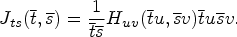
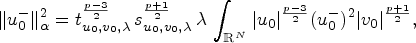
(\binom{H_{s s} (s, t) s^{2} - (1 + ρ) H_{s} (s, t) s H_{s t} (s, t) s t}{H_{s t} (s, t) s t H_{t t} (s, t) t^{2} - (1 + ρ) H_{t} (s, t) t})

(2.8)

is non-positive definite for all

(s, t)

such that

s \neq 0

t \neq 0

. Let

S_{p}

be the sharp constant of the Sobolev embedding

H_{r}^{1} (R^{N}) ↪ L^{p + 1} (R^{N})

‖ u ‖_{α}^{2} \geq S_{p} | u |_{p + 1}^{2}, \forall u \in H_{r}^{1} (R^{N}) .

(2.9)

Lemma 2.4

If for any $u, v \in H_{r}^{1} (R^{N}), u \neq 0, v \neq 0$ ,

\frac{4 | λ |^{2}}{(p + 1)^{2}} (\int_{R^{N}} | u |^{\frac{p + 1}{2}} | v |^{\frac{p + 1}{2}} d x)^{2} \geq μ ν | u |_{p + 1}^{p + 1} | v |_{p + 1}^{p + 1},

(2.10)

then

sup_{t, s \geq 0} Φ_{λ} (t u, s v) = + \infty .

Proof.

Take $r > 0$ such that

\begin{aligned} \frac{2 | λ |}{p + 1} \int_{R^{N}} | u |^{\frac{p + 1}{2}} | v |^{\frac{p + 1}{2}} d x \geq μ r^{\frac{p + 1}{2}} | u |_{p + 1}^{p + 1}, \\ \frac{2 | λ |}{p + 1} \int_{R^{N}} | u |^{\frac{p + 1}{2}} | v |^{\frac{p + 1}{2}} d x \geq \frac{ν}{r^{\frac{p + 1}{2}}} | v |_{p + 1}^{p + 1}, \end{aligned}

then, as

t \to + \infty

, we get

\begin{aligned} Φ_{λ} (r t u, t v) & := \frac{1}{2} t^{2} (r^{2} ‖ u ‖_{α}^{2} + ‖ v ‖_{β}^{2}) - \frac{t^{p + 1}}{p + 1} (μ r^{p + 1} | u |_{p + 1}^{p + 1} + ν | v |_{p + 1}^{p + 1}) \\ + \frac{2 | λ |}{p + 1} r^{\frac{p + 1}{2}} t^{p + 1} \int_{R^{N}} | u |^{\frac{p + 1}{2}} | v |^{\frac{p + 1}{2}} d x \\ \geq \frac{1}{2} t^{2} (r^{2} ‖ u ‖_{α}^{2} + ‖ v ‖_{β}^{2}) - \frac{t^{p + 1}}{p + 1} (μ r^{p + 1} | u |_{p + 1}^{p + 1} + ν | v |_{p + 1}^{p + 1}) \\ + \frac{t^{p + 1}}{2} (μ r^{p + 1} | u |_{p + 1}^{p + 1} + ν | v |_{p + 1}^{p + 1}) \\ \geq \frac{1}{2} t^{2} (r^{2} ‖ u ‖_{α}^{2} + ‖ v ‖_{β}^{2}) \to + \infty . \end{aligned}

The conclusion holds.

Let $(u, v) \in A_{λ}^{*}$ and consider

sup_{t, s > 0} Φ_{λ} (t u, s v) = Φ_{λ} (t_{u, v, λ} u, s_{u, v, λ} v) .

(2.11)

Note that for

t, s > 0

\begin{aligned} Φ_{λ} (t u, s v) & := \frac{1}{2} (t^{2} ‖ u ‖_{α}^{2} + s^{2} ‖ v ‖_{β}^{2}) - \frac{1}{p + 1} (μ t^{p + 1} | u |_{p + 1}^{p + 1} + ν s^{p + 1} | v |_{p + 1}^{p + 1}) \\ + \frac{2 | λ |}{p + 1} t^{\frac{p + 1}{2}} s^{\frac{p + 1}{2}} \int_{R^{N}} | u |^{\frac{p + 1}{2}} | v |^{\frac{p + 1}{2}} d x . \end{aligned}

(2.12)

Fix

(u, v) \in H_{r} ∖ {(0, 0)}

and define

J (t, s) := Φ_{λ} (t u, s v)

. We study the set of critical points of

J

. We will show that there is exactly one critical point with nonzero component (and thus maxima) in the first quadrant.

In fact, let $(\bar{t}, \bar{s})$ be a critical point of $J$ , then

\begin{aligned} \bar{t} (‖ u ‖_{α}^{2} - \frac{μ}{{\bar{t}}^{2}} | \bar{t} u |_{p + 1}^{p + 1} \bar{t} u + \frac{| λ |}{{\bar{t}}^{2}} \int_{R^{N}} H_{u} (\bar{t} u, \bar{s} v) \bar{t} u d x) = 0, \\ \bar{s} (‖ v ‖_{β}^{2} - \frac{ν}{{\bar{s}}^{2}} | \bar{s} v |_{p + 1}^{p + 1} \bar{s} v + \frac{| λ |}{{\bar{s}}^{2}} \int_{R^{N}} H_{v} (\bar{t} u, \bar{s} v) \bar{s} v d x) = 0. \end{aligned}

Let

\bar{t} \neq 0

and

\bar{s} \neq 0

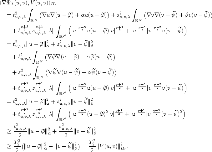
. Define the quadratic form associated to the pair

(\bar{t}, \bar{s})

Q (a, b) = J_{t t} (\bar{t}, \bar{s}) a^{2} + 2 J_{t s} (\bar{t}, \bar{s}) a b + J_{s s} (\bar{t}, \bar{s}) b^{2}, (a, b) \in R^{2} .

We are going to show that

Q (a, b) < 0

for all

(a, b) \in R^{2}

. We estimate the second derivatives

\begin{aligned} J_{t t} (\bar{t}, \bar{s}) & := ‖ u ‖_{α}^{2} - \frac{μ}{{\bar{t}}^{2}} | \bar{t} u |_{p + 1}^{p + 1} + \frac{| λ |}{{\bar{t}}^{2}} \int_{R^{N}} H_{u u} (\bar{t} u, \bar{s} v) {\bar{t}}^{2} u^{2} d x \\ \leq - ρ ‖ u ‖_{α}^{2} + \frac{| λ |}{{\bar{t}}^{2}} \int_{R^{N}} (H_{u u} (\bar{t} u, \bar{s} v) {\bar{t}}^{2} u^{2} - (1 + ρ) H_{u} (\bar{t} u, \bar{s} v) \bar{t} u) d x . \end{aligned}

and

J_{s s} (\bar{t}, \bar{s}) \leq - ρ ‖ v ‖_{β}^{2} + \frac{| λ |}{{\bar{s}}^{2}} \int_{R^{N}} (H_{v v} (\bar{t} u, \bar{s} v) {\bar{s}}^{2} v^{2} - (1 + ρ) H_{v} (\bar{t} u, \bar{s} v) \bar{s} v) d x,

while

J_{t s} (\bar{t}, \bar{s}) = \frac{1}{\bar{t} \bar{s}} H_{u v} (\bar{t} u, \bar{s} v) \bar{t} u \bar{s} v .

Thus we obtain

Q (a, b) \leq - ρ a^{2} ‖ u ‖_{α}^{2} - ρ b^{2} ‖ v ‖_{β}^{2} + Q_{H} (\bar{t} u, \bar{s} v) (a, b),

where the quadratic form

Q_{H}

is negatively definite by assumption (2.8).

Since $J (t, s) \to - \infty$ as $| s | + | t | \to \infty$ , then $J$ must have at least a local maximum in each of the quadrants. $J$ has one local minimum at the origin, providing a local degree $+ 1$ ; $J$ has exactly four critical points with one null component having index $- 1$ . Let $n$ be the number of local maxima, by the excision property of the degree it must hold:

+ 1 = \deg (▽ J, 0, B_{R}) = (+ 1) \cdot 1 + (- 1) \cdot 4 + (+ 1) \cdot n,

that gives

n = 4

, where

B_{R}

is a suitably large ball. Thus there are exactly four critical points with nonzero components and thus maxima, one in each of the quadrant. Now we define

(t_{u, v, λ}, s_{u, v, λ})

as the unique local maximum of

J

in the first quadrant, so

t_{u, v, λ}, s_{u, v, λ}

is unique.

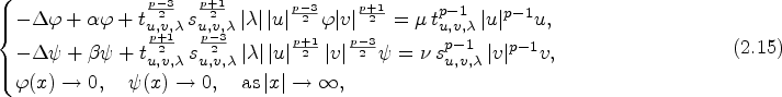
Note that for $t, s \geq 0$ , $1 < p, q < 2^{*} - 1$ , by (2.12), we can choose some positive constant $T$ such that $Φ_{λ} (t u, s v) < 0$ for any $t, s > T$ , therefore, $t_{u, v, λ}, s_{u, v, λ} \in [0, T]$ . By (2.9), for any $(u, v) \in A_{λ}$ ,

\begin{aligned} μ t_{u, v, λ}^{p - 1} | u |_{p + 1}^{p + 1} \geq ‖ u ‖_{α}^{2} \geq S_{p} | u |_{p + 1}^{2}, \\ ν s_{u, v, λ}^{p - 1} | v |_{p + 1}^{p + 1} \geq ‖ v ‖_{β}^{2} \geq S_{p} | v |_{p + 1}^{2} . \end{aligned}

Thus, we obtain

t_{u, v, λ} \geq {(\frac{S_{p}}{μ})}^{\frac{1}{p - 1}} > 0, s_{u, v, λ} \geq {(\frac{S_{p}}{ν})}^{\frac{1}{p - 1}} > 0.

(2.13)

Hence, there exists

T_{1} \geq T_{2} > 0

such that for any

(u, v) \in A_{λ}

T_{2} \leq t_{u, v, λ}, s_{u, v, λ} \leq T_{1} .

(2.14)

For any

(u, v) \in A_{λ}^{*}

, the following linear problem:

{\begin{cases} - Δ φ + α φ + t_{u, v, λ}^{\frac{p - 3}{2}} s_{u, v, λ}^{\frac{p + 1}{2}} | λ | | u |^{\frac{p - 3}{2}} φ | v |^{\frac{p + 1}{2}} = μ t_{u, v, λ}^{p - 1} | u |^{p - 1} u, \\ - Δ ψ + β ψ + t_{u, v, λ}^{\frac{p + 1}{2}} s_{u, v, λ}^{\frac{p - 3}{2}} | λ | | u |^{\frac{p + 1}{2}} | v |^{\frac{p - 3}{2}} ψ = ν s_{u, v, λ}^{p - 1} | v |^{p - 1} v, \\ φ (x) \to 0, ψ (x) \to 0, as | x | \to \infty, \end{cases}

(2.15)

has unique solution

(φ, ψ) \in H ∖ {(0, 0)}

and

\begin{aligned} \int_{R^{N}} | u |^{p - 1} u φ d x = \frac{1}{μ t_{u, v, λ}^{p - 1}} (‖ φ ‖_{α}^{2} + t_{u, v, λ}^{\frac{p - 3}{2}} s_{u, v, λ}^{\frac{p + 1}{2}} | λ | \int_{R^{N}} | u |^{\frac{p - 3}{2}} | φ |^{2} | v |^{\frac{p + 1}{2}} d x) > 0, \\ \int_{R^{N}} | v |^{p - 1} v ψ d x = \frac{1}{ν s_{u, v, λ}^{p - 1}} (‖ ψ ‖_{β}^{2} + t_{u, v, λ}^{\frac{p + 1}{2}} s_{u, v, λ}^{\frac{p - 3}{2}} | λ | \int_{R^{N}} | u |^{\frac{p + 1}{2}} | v |^{\frac{p - 3}{2}} | ψ |^{2} d x) > 0. \end{aligned}

So we can define

a := \frac{1}{\int_{R^{N}} | u |^{p - 1} u φ d x} > 0, b := \frac{1}{\int_{R^{N}} | v |^{p - 1} v ψ d x} > 0,

then

(\tilde{φ}, \tilde{ψ}) := (a φ, b ψ)

is the unique solution of

{\begin{cases} - Δ \tilde{φ} + α \tilde{φ} + t_{u, v, λ}^{\frac{p - 3}{2}} s_{u, v, λ}^{\frac{p + 1}{2}} | λ | | u |^{\frac{p - 3}{2}} \tilde{φ} | v |^{\frac{p + 1}{2}} = a μ t_{u, v, λ}^{p - 1} | u |^{p - 1} u, \\ - Δ \tilde{ψ} + β \tilde{ψ} + t_{u, v, λ}^{\frac{p + 1}{2}} s_{u, v, λ}^{\frac{p - 3}{2}} | λ | | u |^{\frac{p + 1}{2}} | v |^{\frac{p - 3}{2}} \tilde{ψ} = b ν s_{u, v, λ}^{p - 1} | v |^{p - 1} v, \\ \int_{R^{N}} | u |^{p - 1} u \tilde{φ} d x = \int_{R^{N}} | v |^{p - 1} v \tilde{ψ} d x = 1, \\ \tilde{φ} (x) \to 0, \tilde{ψ} (x) \to 0, as | x | \to \infty . \end{cases}

(2.16)

Let

k_{1}, k_{2} \geq 2

. Take nonempty open radially symmetric subsets

Ω_{1}, Ω_{2} \subset R^{N}

with

Ω_{1} \cap Ω_{2} = \emptyset

. Define

\begin{aligned} A_{1} & := {u \in span {U_{1}, \dots, U_{k_{1}}} : U_{i} \in H_{r}^{1} (Ω_{1}), \\ U_{i} are linearly independent, 1 \leq i \leq k_{1}, | u |_{p + 1} = 1}, \end{aligned}

(2.17)

\begin{aligned} A_{2} & := {v \in span {V_{1}, \dots, V_{k_{2}}} : V_{i} \in H_{r}^{1} (Ω_{2}), \\ V_{i} are linearly independent, 1 \leq i \leq k_{2}, | v |_{p + 1} = 1} . \end{aligned}

(2.18)

There is an odd homeomorphism from

S^{k_{i} - 1}

A_{i}

i = 1, 2

. By Lemma

2.2 (1)

, one has

D := A_{1} \times A_{2} \in Γ^{(k_{1}, k_{2})}

. For any

(u, v) \in D

, there holds

u \cdot v \equiv 0

and

(u, v) \in A_{λ}

. Since all the norms of a finite-dimensional linear space are equivalent, there exist constants

d_{k_{i}} > 0, i = 1, 2

such that

‖ u ‖_{α}^{2} \leq d_{k_{1}} | u |_{p + 1}^{2}

and

‖ v ‖_{β}^{2} \leq d_{k_{2}} | v |_{p + 1}^{2}

, hence

\begin{aligned} sup_{A} sup_{t, s \geq 0} Φ_{λ} (t u, s v) & = (\frac{1}{2} - \frac{1}{p + 1}) sup_{A} (t_{u, v, λ}^{2} ‖ u ‖_{α}^{2} + s_{u, v, λ}^{2} ‖ v ‖_{β}^{2}) \\ \leq (\frac{1}{2} - \frac{1}{p + 1}) sup_{A} (t_{u, v, λ}^{2} d_{k_{1}} | u |_{p + 1}^{2} + s_{u, v, λ}^{2} d_{k_{2}} | v |_{p + 1}^{2}) \\ \leq d^{k_{1}, k_{2}} . \end{aligned}

Define

Γ_{λ}^{(k_{1}, k_{2})} := {A \in Γ^{(k_{1}, k_{2})} : sup_{A} sup_{t, s \geq 0} Φ_{λ} (t u, s v) < d^{k_{1}, k_{2}} + 1} .

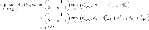
Observe that

Γ_{λ}^{(k_{1}, k_{2})} \neq \emptyset

Γ_{λ}^{(k_{1}, k_{2})} \subset Γ_{λ}^{(k_{1}^{'}, k_{2}^{'})}

when

k_{1} \geq k_{1}^{'}

and

k_{2} \geq k_{2}^{'}

. We are now ready to define a sequence of minimax energy levels which will turn out to be critical levels for

Φ_{λ}

over

A

. For every

k_{1}, k_{2} \geq 2

and

0 < δ < 2^{- \frac{1}{p + 1}}

, define

d_{λ, δ}^{k_{1}, k_{2}} := inf_{A \in Γ_{λ}^{(k_{1}, k_{2})}} sup_{A ∖ P_{δ}} sup_{t, s \geq 0} Φ_{λ} (t u, s v) .

(2.19)

It is easy to see that for any

k_{1}, k_{2} \geq 2

λ < 0

and

0 < δ < 2^{- \frac{1}{p + 1}}

, there holds

d_{λ, δ}^{k_{1}, k_{2}} \leq d^{k_{1}, k_{2}},

(2.20)

and

sup_{t, s \geq 0} Φ_{λ} (t u, s v)

is continuous on

A^{*}

. Moreover,

\begin{aligned} inf_{A^{*}} sup_{t, s \geq 0} Φ_{λ} (t u, s v) & = (\frac{1}{2} - \frac{1}{p + 1}) inf_{A^{*}} (t_{u, v, λ}^{2} ‖ u ‖_{α}^{2} + s_{u, v, λ}^{2} ‖ v ‖_{β}^{2}) \\ \geq (\frac{1}{2} - \frac{1}{p + 1}) inf_{A^{*}} (t_{u, v, λ}^{2} S_{p} | u |_{p + 1}^{2} + s_{u, v, λ}^{2} S_{p} | v |_{p + 1}^{2}) \\ \geq C > 0. \end{aligned}

therefore,

d_{λ, δ}^{k_{1}, k_{2}} \geq C > 0

As a step towards to the proof of Theorem 1.1, we will prove that $d_{λ, δ}^{k_{1}, k_{2}}$ is indeed a critical level of $Φ_{λ}$ for $δ$ sufficiently small. In order to prove Theorem 1.1, it is necessary to find a pseudogradient for $Φ_{λ}$ over $A$ for which $P_{δ}$ is positively invariant for the associated flow. We can now define the operator

K : A_{λ}^{*} \to H; (u, v) \mapsto (\tilde{φ}, \tilde{ψ}),

that is, for any

(u, v)

K (u, v) = (\tilde{φ}, \tilde{ψ})

is the unique solution of (2.16). It is easy to prove that

K (σ_{i} (u, v)) = σ_{i} (K (u, v))

i = 1, 2

Now, we give some property of the operator $K$ . We can now prove that $K$ is a compact $C^{1}$ operator.

Lemma 2.5

The operator $K$ is of class $C^{1}$ .

Proof.

Define $C^{1}$ map $J_{i} : A_{λ}^{*} \times H^{1} (R^{N}) \times R \to H^{1} (R^{N}) \times R$ , $i = 1, 2$ , by

\begin{aligned} J_{1} ((u, v), ω, γ) \\ = (ω - (- Δ + α)^{- 1} (t_{u, v, λ}^{\frac{p - 3}{2}} s_{u, v, λ}^{\frac{p + 1}{2}} | λ | | u |^{\frac{p - 3}{2}} ω | v |^{\frac{p + 1}{2}} + γ μ t_{u, v, λ}^{p - 1} | u |^{p - 1} u), \\ \int_{R^{N}} | u |^{p - 1} u ω d x - 1) \end{aligned}

and

\begin{aligned} J_{2} ((u, v), ω, γ) \\ = (ω - (- Δ + β)^{- 1} (t_{u, v, λ}^{\frac{p + 1}{2}} s_{u, v, λ}^{\frac{p - 3}{2}} | λ | | u |^{\frac{p + 1}{2}} | v |^{\frac{p - 3}{2}} ω + γ ν s_{u, v, λ}^{p - 1} | v |^{p - 1} v), \\ \int_{R^{N}} | v |^{p - 1} v ω d x - 1) \end{aligned}

then by (2.16),

J_{1} ((u, v), \tilde{φ}, a) = J_{2} ((u, v), \tilde{ψ}, b) = 0

. Moreover, the derivatives of

J_{1}

and

J_{2}

with respect to

(ω, γ)

at the point

((u, v), \tilde{φ}, a)

and

((u, v), \tilde{ψ}, b)

in the direction

(ω_{0}, γ_{0})

, respectively, are

\begin{aligned} D_{ω, γ} J_{1} ((u, v), \tilde{φ}, a) (ω_{0}, γ_{0}) \\ = (ω_{0} - (- Δ + α)^{- 1} (t_{u, v, λ}^{\frac{p - 3}{2}} s_{u, v, λ}^{\frac{p + 1}{2}} | λ | | u |^{\frac{p - 3}{2}} ω_{0} | v |^{\frac{p + 1}{2}} + γ_{0} μ t_{u, v, λ}^{p - 1} | u |^{p - 1} u), \\ \int_{R^{N}} | u |^{p - 1} u ω_{0} d x) \end{aligned}

and

\begin{aligned} D_{ω, γ} J_{2} ((u, v), \tilde{ψ}, b) (ω_{0}, γ_{0}) \\ = (ω_{0} - (- Δ + β)^{- 1} (t_{u, v, λ}^{\frac{p + 1}{2}} s_{u, v, λ}^{\frac{p - 3}{2}} | λ | | u |^{\frac{p + 1}{2}} | v |^{\frac{p - 3}{2}} ω_{0} + γ_{0} ν s_{u, v, λ}^{p - 1} | v |^{p - 1} v), \\ \int_{R^{N}} | v |^{p - 1} v ω_{0} d x) \end{aligned}

We claim that

D_{ω, γ} J_{1} ((u, v), \tilde{φ}, a)

and

D_{ω, γ} J_{2} ((u, v), \tilde{ψ}, b)

are bijective maps. In fact, for any

(ω, γ) \in H_{r}^{1} (R^{N}) \times R

, the following linear problems:

\begin{aligned} - Δ ω_{1} + α ω_{1} - t_{u, v, λ}^{\frac{p - 3}{2}} s_{u, v, λ}^{\frac{p + 1}{2}} | λ | | u |^{\frac{p - 3}{2}} ω_{1} | v |^{\frac{p + 1}{2}} = - Δ ω + α ω, \\ - Δ ω_{2} + α ω_{2} - t_{u, v, λ}^{\frac{p - 3}{2}} s_{u, v, λ}^{\frac{p + 1}{2}} | λ | | u |^{\frac{p - 3}{2}} ω_{2} | v |^{\frac{p + 1}{2}} = μ t_{u, v, λ}^{p - 1} | u |^{p - 1} u, \end{aligned}

have unique solutions

ω_{1}, ω_{2} \in H_{r}^{1} (R^{N})

ω_{2} \neq 0

u \in A_{λ}^{*}

, then we define

γ_{0} = \frac{γ - \int_{R^{N}} | u |^{p - 1} u ω_{1} d x}{\int_{R^{N}} | u |^{p - 1} u ω_{2} d x},

we have

D_{ω, γ} J_{1} ((u, v), \tilde{φ}, a) (ω_{1} + γ_{0} ω_{2}, γ_{0}) = (ω, γ),

D_{ω, γ} J_{1} ((u, v), \tilde{φ}, a)

is surjective. Similarly,

D_{ω, γ} J_{2} ((u, v), \tilde{ψ}, b)

is surjective.

If $D_{ω, γ} J_{1} ((u, v), \tilde{φ}, a) (ω_{0}, γ_{0}) = (0, 0)$ , then

{\begin{cases} - Δ ω_{0} + α ω_{0} = t_{u, v, λ}^{\frac{p - 3}{2}} s_{u, v, λ}^{\frac{p + 1}{2}} | λ | | u |^{\frac{p - 3}{2}} ω_{0} | v |^{\frac{p + 1}{2}} + γ_{0} μ t_{u, v, λ}^{p - 1} | u |^{p - 1} u, \\ \int_{R^{N}} | u |^{p - 1} u ω_{0} d x = 0, \end{cases}

ω_{0} \equiv 0

γ_{0} μ t_{u, v, λ}^{p - 1} | u |^{p - 1} u \equiv 0

, by

t_{u, v, λ} > 0

u \in A_{λ}^{*}

, we have

γ_{0} = 0

, this implies

D_{ω, γ} J_{1} ((u, v), \tilde{φ}, a)

is injective. Therefore,

D_{ω, γ} J_{1} ((u, v), \tilde{φ}, a)

is bijective. Similarly,

D_{ω, γ} J_{2} ((u, v), \tilde{ψ}, b)

is bijective map. Then we can apply the implicit function theorem to the

C^{1}

maps

D_{ω, γ} J_{1} ((u, v), \tilde{φ}, a)

and

D_{ω, γ} J_{2} ((u, v), \tilde{ψ}, b)

, we have the conclusions.

Lemma 2.6

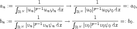
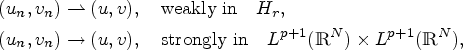
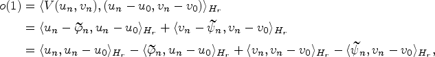
Let ${(u_{n}, v_{n})}_{n \geq 1} \subset A_{λ}$ be bounded in $H_{r}$ . Then there exists $({\tilde{φ}}_{0}, {\tilde{ψ}}_{0}) \in H_{r}$ such that, up to a subsequence,

K (u_{n}, v_{n}) \to ({\tilde{φ}}_{0}, {\tilde{ψ}}_{0}), strongly\, in H_{r} .

Proof.

Since ${(u_{n}, v_{n})}_{n \geq 1} \subset A_{λ}$ is bounded in $H_{r}$ , we have

\begin{aligned} (u_{n}, v_{n}) ⇀ (u_{0}, v_{0}), weakly in H_{r}, \\ (u_{n}, v_{n}) \to (u_{0}, v_{0}), strongly in L^{p + 1} (R^{N}) \times L^{p + 1} (R^{N}), \end{aligned}

and

| u_{0} |_{p + 1} = | v_{0} |_{p + 1} = 1

(u_{0}, v_{0}) \in A_{λ}

. Then by (2.9), (2.14) and (2.15), we have

\begin{aligned} ‖ φ_{n} ‖_{α}^{2} & \leq μ t_{u_{n}, v_{n}, λ}^{p - 1} \int_{R^{N}} | u_{n} |^{p - 1} u_{n} φ_{n} d x \\ \leq μ t_{u_{n}, v_{n}, λ}^{p - 1} | u_{n} |_{p + 1}^{p} | φ_{n} |_{p + 1} \leq C | φ_{n} |_{p + 1} \leq C ‖ φ_{n} ‖_{α} . \end{aligned}

Similar estimates hold for

ψ_{n}

, we get

‖ ψ_{n} ‖_{β}^{2} \leq C ‖ ψ_{n} ‖_{β}

, so

{(φ_{n}, ψ_{n})}_{n \geq 1} \subset H_{r}

are bounded. Thus

\begin{aligned} (φ_{n}, ψ_{n}) ⇀ (φ_{0}, ψ_{0}), weakly in H_{r}, \\ (φ_{n}, ψ_{n}) \to (φ_{0}, ψ_{0}), strongly in L^{p + 1} (R^{N}) \times L^{p + 1} (R^{N}) . \end{aligned}

Then by (2.15) and H

\ddot{o}

lder inequality, as

n \to \infty

\begin{aligned} \int_{R^{N}} (\nabla φ_{n} \nabla (φ_{n} - φ_{0}) + α φ_{n} (φ_{n} - φ_{0})) d x \\ = - t_{u_{n}, v_{n}, λ}^{\frac{p - 3}{2}} s_{u_{n}, v_{n}, λ}^{\frac{p + 1}{2}} | λ | \int_{R^{N}} | u_{n} |^{\frac{p - 3}{2}} φ_{n} (φ_{n} - φ_{0}) | v_{n} |^{\frac{p + 1}{2}} d x \\ + μ t_{u_{n}, v_{n}, λ}^{p - 1} \int_{R^{N}} | u_{n} |^{p - 1} u_{n} (φ_{n} - φ_{0}) d x \to 0. \end{aligned}

Hence,

‖ φ_{n} ‖_{α}^{2} = \int_{R^{N}} (\nabla φ_{n} \nabla φ_{0} + α φ_{n} φ_{0}) d x + o (1) = ‖ φ_{0} ‖_{α}^{2} + o (1) .

Similarly, we have

‖ ψ_{n} ‖_{β}^{2} = ‖ ψ_{0} ‖_{β}^{2} + o (1)

. Therefore, we have

(φ_{n}, ψ_{n}) \to (φ_{0}, ψ_{0})

strongly in

H_{r}

and

(φ_{0}, ψ_{0})

satisfies

{\begin{cases} - Δ φ_{0} + α φ_{0} + t_{u_{0}, v_{0}, λ}^{\frac{p - 3}{2}} s_{u_{0}, v_{0}, λ}^{\frac{p + 1}{2}} | λ | | u_{0} |^{\frac{p - 3}{2}} φ_{0} | v_{0} |^{\frac{p + 1}{2}} = μ t_{u_{0}, v_{0}, λ}^{p - 1} | u_{0} |^{p - 1} u_{0}, \\ - Δ ψ_{0} + β ψ_{0} + t_{u_{0}, v_{0}, λ}^{\frac{p + 1}{2}} s_{u_{0}, v_{0}, λ}^{\frac{p - 3}{2}} | λ | | u_{0} |^{\frac{p + 1}{2}} | v_{0} |^{\frac{p - 3}{2}} ψ_{0} = ν s_{u_{0}, v_{0}, λ}^{p - 1} | v_{0} |^{p - 1} v_{0}, \\ φ_{0} (x) \to 0, ψ_{0} (x) \to 0, as | x | \to \infty . \end{cases}

Since

| u_{0} |_{p + 1} = | v_{0} |_{p + 1} = 1

, so

φ_{0} \neq 0

ψ_{0} \neq 0

and

\begin{aligned} a_{n} := \frac{1}{\int_{R^{N}} | u_{n} |^{p - 1} u_{n} φ_{n} d x} \to \frac{1}{\int_{R^{N}} | u_{0} |^{p - 1} u_{0} φ_{0} d x} =: a_{0}, \\ b_{n} := \frac{1}{\int_{R^{N}} | v_{n} |^{p - 1} v_{n} ψ_{n} d x} \to \frac{1}{\int_{R^{N}} | v_{0} |^{p - 1} v_{0} ψ_{0} d x} =: b_{0} . \end{aligned}

We see that

\begin{aligned} {\tilde{φ}}_{n} = a_{n} φ_{n} \to a_{0} φ_{0} =: {\tilde{φ}}_{0}, strongly in H_{r}^{1} (R^{N}), \\ {\tilde{ψ}}_{n} = b_{n} ψ_{n} \to b_{0} ψ_{0} =: {\tilde{ψ}}_{0}, strongly in H_{r}^{1} (R^{N}) . \end{aligned}

This completes the proof.

Lemma 2.7

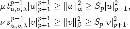
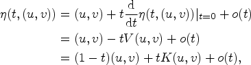
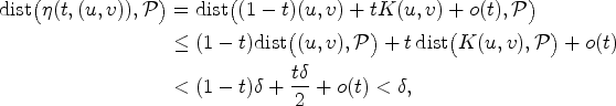
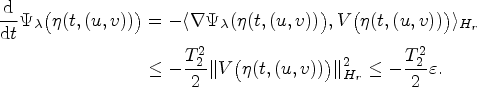
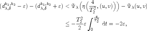
For any $0 < δ < 2^{- \frac{1}{p + 1}}$ sufficiently small, $(u, v) \in A$ satisfying $sup_{t, s \geq 0} Φ_{λ} (t u, s v) < d^{k_{1}, k_{2}} + 1$ , $dist ((u, v), P) < δ$ , then there holds

dist (K (u, v), P) < \frac{δ}{2} .

Proof.

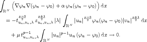
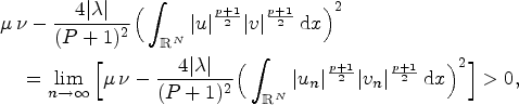
Suppose by contradiction that there exists $δ_{n} \to 0$ and $(u_{n}, v_{n}) \in A$ satisfying $sup_{t, s \geq 0} Φ_{λ} (t u_{n}, s v_{n}) < d^{k_{1}, k_{2}} + 1$ , $dist ((u_{n}, v_{n}), P) < δ_{n}$ and $dist (K (u_{n}, v_{n}), P) \geq \frac{δ_{n}}{2}$ . We suppose that $dist ((u_{n}, v_{n}), P) = | u_{n}^{-} |_{p + 1},$ without loss of generality. Then $(u_{n}, v_{n}) \in A_{λ}$ and

sup_{t, s \geq 0} Φ_{λ} (t u_{n}, s v_{n}) = (\frac{1}{2} - \frac{1}{p + 1}) (t_{u, v, λ}^{2} ‖ u_{n} ‖_{α}^{2} + s_{u, v, λ}^{2} ‖ v_{n} ‖_{β}^{2}) < d^{k_{1}, k_{2}} + 1,

we get that

{(u_{n}, v_{n})}_{n \geq 1}

are bounded in

H_{r}

, we have

\begin{aligned} (u_{n}, v_{n}) ⇀ (u, v), weakly in H_{r}, \\ (u_{n}, v_{n}) \to (u, v), strongly in L^{p + 1} (R^{N}) \times L^{p + 1} (R^{N}), \end{aligned}

and

(u, v) \in A

. Moreover,

\begin{aligned} μ ν - \frac{4 | λ |}{(P + 1)^{2}} (\int_{R^{N}} | u |^{\frac{p + 1}{2}} | v |^{\frac{p + 1}{2}} d x)^{2} \\ = lim_{n \to \infty} [μ ν - \frac{4 | λ |}{(P + 1)^{2}} (\int_{R^{N}} | u_{n} |^{\frac{p + 1}{2}} | v_{n} |^{\frac{p + 1}{2}} d x)^{2}] > 0, \end{aligned}

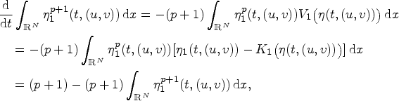
so we have

(u, v) \in A_{λ}

. This together with (2.9) and (2.16) allow us to get

\begin{aligned} | {\tilde{φ}}_{n}^{-} |_{p + 1}^{2} \leq \frac{1}{S_{p}} ‖ {\tilde{φ}}_{n}^{-} ‖_{α}^{2} \\ \leq \frac{1}{S_{p}} (‖ {\tilde{φ}}_{n}^{-} ‖_{α}^{2} + t_{u_{n}, v_{n}, λ}^{\frac{p - 3}{2}} s_{u_{n}, v_{n}, λ}^{\frac{p + 1}{2}} | λ | \int_{R^{N}} | u_{n} |^{\frac{p - 3}{2}} ({\tilde{φ}}_{n}^{-})^{2} | v_{n} |^{\frac{p + 1}{2}} d x) \\ = - \frac{1}{S_{p}} a_{n} μ_{n} t_{u_{n}, v_{n}, λ}^{p - 1} \int_{R^{N}} | u_{n} |^{p - 1} u_{n} {\tilde{φ}}_{n}^{-} d x \\ \leq C \int_{R^{N}} (u_{n}^{-})^{p} {\tilde{φ}}_{n}^{-} d x \leq C | u_{n}^{-} |_{p + 1}^{p} | {\tilde{φ}}_{n}^{-} |_{p + 1} \leq C δ_{n}^{p} | {\tilde{φ}}_{n}^{-} |_{p + 1} \end{aligned}

and hence

dist (K (u_{n}, v_{n}), P) \leq | {\tilde{φ}}_{n}^{-} |_{p + 1} \leq C δ_{n}^{p} < \frac{δ_{n}}{2}

for

n

sufficiently large, which is a contradiction. This completes the proof.

Now define a map

V : A_{λ}^{*} \to H; (u, v) \mapsto (u, v) - K (u, v) .

It is easy to prove that

V (σ_{i} (u, v)) = σ_{i} (V (u, v))

i = 1, 2

. We will prove that if

(u, v) \in A_{λ} ∖ P

V (u, v) = 0

, then

(t_{u, v, λ} u, s_{u, v, λ} v)

is a sign-changing solution of equation (2.1). Firstly, we prove that

V

satisfied the Palais-Smale type condition and

V

is a pseudogradient for

sup_{t, s \geq 0} Φ_{λ} (t u, s v)

over

A_{λ}

. Denote

Ψ_{λ} (u, v) := sup_{t, s \geq 0} Φ_{λ} (t u, s v) .

(2.21)

Lemma 2.8

(Palais-Smale Type Condition) Let $(u_{n}, v_{n}) \in A_{λ}$ be such that

Ψ_{λ} (u_{n}, v_{n}) \to c < d^{k_{1}, k_{2}} + 1 and V (u_{n}, v_{n}) \to 0 strongly in H .

Then there exists

(u_{0}, v_{0}) \in A_{λ}

such that, up to a subsequence,

(u_{n}, v_{n}) \to (u_{0}, v_{0})

strongly in

H_{r}

and

V (u_{0}, v_{0}) = 0

. We also have

⟨ \nabla Ψ_{λ} (u, v), V (u, v) ⟩_{H_{r}} \geq \frac{T_{2}^{2}}{2} ‖ V (u, v) ‖_{H_{r}}^{2}, \forall (u, v) \in A_{λ} .

Proof.

Similar as Lemma 2.6, we have, up to a subsequence,

\begin{aligned} (u_{n}, v_{n}) ⇀ (u_{0}, v_{0}), weakly in H_{r}, \\ K (u_{n}, v_{n}) \to ({\tilde{φ}}_{0}, {\tilde{ψ}}_{0}), strongly in H_{r} . \end{aligned}

Then we have, as

n \to \infty

\begin{aligned} o (1) & = ⟨ V (u_{n}, v_{n}), (u_{n} - u_{0}, v_{n} - v_{0}) ⟩_{H_{r}} \\ = ⟨ u_{n} - {\tilde{φ}}_{n}, u_{n} - u_{0} ⟩_{H_{r}} + ⟨ v_{n} - {\tilde{ψ}}_{n}, v_{n} - v_{0} ⟩_{H_{r}} \\ = ⟨ u_{n}, u_{n} - u_{0} ⟩_{H_{r}} - ⟨ {\tilde{φ}}_{n}, u_{n} - u_{0} ⟩_{H_{r}} + ⟨ v_{n}, v_{n} - v_{0} ⟩_{H_{r}} - ⟨ {\tilde{ψ}}_{n}, v_{n} - v_{0} ⟩_{H_{r}}, \end{aligned}

whence

⟨ u_{n}, u_{n} - u_{0} ⟩_{H_{r}} + ⟨ v_{n}, v_{n} - v_{0} ⟩_{H_{r}} = o (1) .

Then

(u_{n}, v_{n}) \to (u_{0}, v_{0})

strongly in

H_{r}

and

(u_{0}, v_{0}) \in {\bar{A}}_{λ}

Φ_{λ} (t_{u_{0}, v_{0}, λ} u_{0}, s_{u_{0}, v_{0}, λ} v_{0}) = lim_{n \to \infty} Φ_{λ} (t_{u_{n}, v_{n}, λ} u_{n}, s_{u_{n}, v_{n}, λ} v_{n}) = c < d^{k_{1}, k_{2}} + 1,

then we have

(u_{0}, v_{0}) \in A_{λ}

V (u_{0}, v_{0}) = lim_{n \to \infty} V (u_{n}, v_{n}) = 0

Finally, we prove that $V$ is a pseudogradient for $Ψ_{λ} (u, v)$ over $A_{λ}$ . Recalling (2.7) and (2.16), it is easy to see that

\int_{R^{N}} | u |^{p - 1} u (u - \tilde{φ}) d x = \int_{R^{N}} | v |^{q - 1} v (v - \tilde{ψ}) d x = 1 - 1 = 0.

Then, by (2.13) and (2.16),

\begin{aligned} ⟨ \nabla Ψ_{λ} (u, v), V (u, v) ⟩_{H_{r}} \\ = t_{u, v, λ}^{2} \int_{R^{N}} (\nabla u \nabla (u - \tilde{φ}) + α u (u - \tilde{φ})) + s_{u, v, λ}^{2} \int_{R^{N}} (\nabla v \nabla (v - \tilde{ψ}) + β v (v - \tilde{ψ})) \\ + t_{u, v, λ}^{\frac{p + 1}{2}} s_{u, v, λ}^{\frac{p + 1}{2}} | λ | \int_{R^{N}} (| u |^{\frac{p - 3}{2}} u (u - \tilde{φ}) | v |^{\frac{p + 1}{2}} + | u |^{\frac{p + 1}{2}} | v |^{\frac{p - 3}{2}} v (v - \tilde{ψ})) \\ = t_{u, v, λ}^{2} ‖ u - \tilde{φ} ‖_{α}^{2} + s_{u, v, λ}^{2} ‖ v - \tilde{ψ} ‖_{β}^{2} \\ + t_{u, v, λ}^{2} \int_{R^{N}} (\nabla \tilde{φ} \nabla (u - \tilde{φ}) + α \tilde{φ} (u - \tilde{φ})) \\ + s_{u, v, λ}^{2} \int_{R^{N}} (\nabla \tilde{ψ} \nabla (u - \tilde{ψ}) + α \tilde{ψ} (v - \tilde{ψ})) \\ + t_{u, v, λ}^{\frac{p + 1}{2}} s_{u, v, λ}^{\frac{p + 1}{2}} | λ | \int_{R^{N}} (| u |^{\frac{p - 3}{2}} u (u - \tilde{φ}) | v |^{\frac{p + 1}{2}} + | u |^{\frac{p + 1}{2}} | v |^{\frac{p - 3}{2}} v (v - \tilde{ψ})) \\ = t_{u, v, λ}^{2} ‖ u - \tilde{φ} ‖_{α}^{2} + s_{u, v, λ}^{2} ‖ v - \tilde{ψ} ‖_{β}^{2} \\ + t_{u, v, λ}^{\frac{p + 1}{2}} s_{u, v, λ}^{\frac{q + 1}{2}} | λ | \int_{R^{N}} (| u |^{\frac{p - 3}{2}} (u - \tilde{φ})^{2} | v |^{\frac{q + 1}{2}} + | u |^{\frac{p + 1}{2}} | v |^{\frac{q - 3}{2}} (v - \tilde{ψ})^{2}) \\ \geq \frac{t_{u, v, λ}^{2}}{2} ‖ u - \tilde{φ} ‖_{α}^{2} + \frac{s_{u, v, λ}^{2}}{2} ‖ v - \tilde{ψ} ‖_{β}^{2} \\ \geq \frac{T_{2}^{2}}{2} (‖ u - \tilde{φ} ‖_{α}^{2} + ‖ v - \tilde{ψ} ‖_{β}^{2}) = \frac{T_{2}^{2}}{2} ‖ V (u, v) ‖_{H_{r}}^{2} . \end{aligned}

This completes the proof.

Lemma 2.9

There exists a unique global solution $η = (η_{1}, η_{2}) : R^{+} \times A_{λ} \to H$ for the initial value problem

{\begin{cases} \frac{d}{d t} η (t, (u, v)) = - V (η (t, (u, v))), \\ η (0, (u, v)) = (u, v) \in A_{λ} . \end{cases}

(2.22)

Moreover,

(1)

for any $t > 0$ and $(u, v) \in A_{λ}$ , there holds $η (t, (u, v)) \in A_{λ}$ ;

(2)

for any $t > 0$ and $(u, v) \in A_{λ}$ , there holds $η (t, σ_{i} (u, v)) = σ_{i} (η (t, (u, v)))$ , $i = 1, 2$ ;

(3)

for any $(u, v) \in A_{λ}$ , $Ψ_{λ} (η (t, (u, v)))$ is nonincreasing in $t$ ;

(4)

there exists $δ_{0} \in (0, 2^{- \frac{1}{p + 1}})$ such that, for any $0 < δ < δ_{0}$ , $(u, v) \in A_{λ} \cap P_{δ}$ and $t > 0$ , there holds $η (t, (u, v)) \in P_{δ}$ .

Proof.

It follows from Lemma 2.5 that $V \in C^{1} (A_{λ}^{*}, H_{r})$ . As $A_{λ} \subset A_{λ}^{*}$ , we get that $V \in C^{1} (A_{λ}, H_{r})$ , then there exists a solution $η : [0, T_{max}) \times A_{λ} \to H_{r}$ , where $T_{max}$ is the maximal time such that (2.22) has a solution $η \in A_{λ}^{*}$ .

For any $(u, v) \in A_{λ}$ and $t \in (0, T_{max})$ , there holds

\begin{aligned} \frac{d}{d t} \int_{R^{N}} η_{1}^{p + 1} (t, (u, v)) d x = - (p + 1) \int_{R^{N}} η_{1}^{p} (t, (u, v)) V_{1} (η (t, (u, v))) d x \\ = - (p + 1) \int_{R^{N}} η_{1}^{p} (t, (u, v)) [η_{1} (t, (u, v)) - K_{1} (η (t, (u, v)))] d x \\ = (p + 1) - (p + 1) \int_{R^{N}} η_{1}^{p + 1} (t, (u, v)) d x, \end{aligned}

so we have

\frac{d}{d t} [e^{(p + 1) t} (\int_{R^{N}} η_{1}^{p + 1} (t, (u, v)) d x - 1)] = 0.

Recall

\int_{R^{N}} η_{1}^{p + 1} (0, (u, v)) d x = \int_{R^{N}} u^{p + 1} d x = 1

, it is easy seen that for any

t \in [0, T_{max})

\int_{R^{N}} η_{1}^{p + 1} (t, (u, v)) d x \equiv \int_{R^{N}} η_{2}^{p + 1} (t, (u, v)) d x \equiv 1.

Thus for any

t \in [0, T_{max})

(u, v) \in A_{λ}

, we have

η (t, (u, v)) \in A_{λ}^{*} \cap A = A_{λ} .

T_{max} < + \infty

, then

η (T_{max}, (u, v)) \in A ∖ A_{λ}^{*}

lim_{t \to T_{max}} ‖ η (t, (u, v)) ‖_{H_{r}} = + \infty

. By Lemma 2.8, we have

\begin{aligned} Ψ_{λ} (η (T_{max}, (u, v))) \\ = Ψ_{λ} (η (0, (u, v))) + \int_{0}^{T_{max}} \frac{d}{d t} Ψ_{λ} (η (t, (u, v))) d t \\ = Ψ_{λ} (u, v) - \int_{0}^{T_{max}} ⟨ \nabla Ψ_{λ} (η (t, (u, v))), V (η (t, (u, v)) ⟩_{H_{r}} d t \\ \leq Ψ_{λ} (u, v) - \frac{T_{2}^{2}}{2} \int_{0}^{T_{max}} ‖ V (η (t, (u, v))) ‖_{H_{r}}^{2} d t \\ \leq Ψ_{λ} (u, v) < + \infty, \end{aligned}

it yields a contradiction with Lemma 2.4. Therefore,

lim_{t \to T_{max}} ‖ η (t, (u, v)) ‖_{H_{r}} = + \infty

. Moreover,

\begin{aligned} \frac{d}{d t} Ψ_{λ} (η (t, (u, v))) & = ⟨ \nabla Ψ_{λ} (η (t, (u, v))), \frac{d}{d t} η (t, (u, v)) ⟩_{H_{r}} \\ = - ⟨ \nabla Ψ_{λ} (η (t, (u, v))), V (η (t, (u, v))) ⟩_{H_{r}} \\ \leq - \frac{T_{2}^{2}}{2} ‖ V (η (t, (u, v))) ‖_{H_{r}}^{2} \leq 0. \end{aligned}

(2.23)

Then for any

t \in [0, T_{max})

, we have

\begin{aligned} (\frac{1}{2} - \frac{1}{p + 1}) (t_{η_{1}, η_{2}, λ}^{2} ‖ η_{1} (t, (u, v)) ‖_{α}^{2} + s_{η_{1}, η_{2}, λ}^{2} ‖ η_{2} (t, (u, v)) ‖_{β}^{2}) \\ = Ψ_{λ} (η (t, (u, v))) \leq Ψ_{λ} (u, v) < + \infty, \end{aligned}

it yields a contradiction. Hence

T_{max} = + \infty

and

η (t, (u, v)) \in A_{λ}

. Thus

(1)

and

(3)

hold. Since

V (σ_{i} (u, v)) = σ_{i} (V (u, v))

i = 1, 2

, then

(2)

holds.

Take $δ_{0} > 0$ as in Lemma 2.7, note that as $t \to 0$ ,

\begin{aligned} η (t, (u, v)) & = (u, v) + t \frac{d}{d t} η (t, (u, v)) |_{t = 0} + o (t) \\ = (u, v) - t V (u, v) + o (t) \\ = (1 - t) (u, v) + t K (u, v) + o (t), \end{aligned}

hence for any

0 < δ < δ_{0}

(u, v) \in A_{λ} \cap P_{δ}

, we have

\begin{aligned} dist (η (t, (u, v)), P) & = dist ((1 - t) (u, v) + t K (u, v) + o (t), P) \\ \leq (1 - t) dist ((u, v), P) + t dist (K (u, v), P) + o (t) \\ < (1 - t) δ + \frac{t δ}{2} + o (t) < δ, \end{aligned}

for sufficiently small

t > 0

, and

(4)

holds. This completes the proof.

In order to prove Theorem 1.1, we will prove that $d_{λ, δ}^{k_{1}, k_{2}}$ is indeed critical energy level for $δ > 0$ sufficiently small.

Lemma 2.10

For any $0 < δ < δ_{0}$ , $k_{1}, k_{2} \geq 2$ , there exists $({\tilde{u}}_{0}, {\tilde{v}}_{0}) \in H_{r}$ such that $({\tilde{u}}_{0}, {\tilde{v}}_{0})$ is a sign-changing solution of equation (2.1) and $Φ_{λ} ({\tilde{u}}_{0}, {\tilde{v}}_{0}) = d_{λ, δ}^{k_{1}, k_{2}}$ .

Proof.

By (2.20), we see that $d_{λ, δ}^{k_{1}, k_{2}} < d^{k_{1}, k_{2}} + 1$ . Assume $0 < ε < 1$ such that for any $(u, v) \in A_{λ}$ , $| Ψ_{λ} (u, v) - d_{λ, δ}^{k_{1}, k_{2}} | \leq 2 ε$ , $dist ((u, v), P) \geq δ$ , there holds $‖ V (u, v) ‖_{H_{r}}^{2} \geq ε$ . By (2.19), there exists $A \in Γ_{λ}^{(k_{1}, k_{2})}$ such that

sup_{A ∖ P_{δ}} Ψ_{λ} (u, v) < d_{λ, δ}^{k_{1}, k_{2}} + ε,

(2.24)

then

sup_{A} Ψ_{λ} (u, v) < d^{k_{1}, k_{2}} + 1

A \subset A_{λ}

. Thus we consider the set

A_{0} = η (\frac{4}{T_{2}^{2}}, A)

A_{0} \in A_{λ}

by Lemma 2.9-

(1)

. From Lemmas 2.2-

(2)

, 2.3, and 2.9-(3), we get

sup_{A_{0}} Ψ_{λ} (u, v) \leq sup_{A} Ψ_{λ} (u, v) < d^{k_{1}, k_{2}} + 1,

A_{0} \in Γ_{λ}^{(k_{1}, k_{2})}

and

A_{0} ∖ P_{δ} \neq \emptyset

. Then by

(2.15), (2.19)

, and Lemma 2.9-(3), for the

ε > 0

t \in [0, \frac{4}{T_{2}^{2}}]

, there exists

(u, v) \in A

such that

η (\frac{4}{T_{2}^{2}}, (u, v)) \in A_{0} ∖ P_{δ}

satisfying

\begin{aligned} d_{λ, δ}^{k_{1}, k_{2}} & \leq sup_{A_{0} ∖ P_{δ}} Ψ_{λ} (u, v) < Ψ_{λ} (η (\frac{4}{T_{2}^{2}}, (u, v))) + ε \\ \leq Ψ_{λ} (η (t, (u, v))) + ε \leq Ψ_{λ} (u, v) + ε < d_{λ, δ}^{k_{1}, k_{2}} + 2 ε . \end{aligned}

(2.25)

We conclude that

‖ V (η (t, (u, v))) ‖_{H_{r}}^{2} \geq ε

for any

t \in [0, \frac{4}{T_{2}^{2}}]

and

\begin{aligned} \frac{d}{d t} Ψ_{λ} (η (t, (u, v))) & = - ⟨ \nabla Ψ_{λ} (η (t, (u, v))), V (η (t, (u, v))) ⟩_{H_{r}} \\ \leq - \frac{T_{2}^{2}}{2} ‖ V (η (t, (u, v))) ‖_{H_{r}}^{2} \leq - \frac{T_{2}^{2}}{2} ε . \end{aligned}

Therefore, by integrating over

[0, \frac{4}{T_{2}^{2}}]

and (2.25), we have

\begin{aligned} (d_{λ, δ}^{k_{1}, k_{2}} - ε) - (d_{λ, δ}^{k_{1}, k_{2}} + ε) & < Ψ_{λ} (η (\frac{4}{T_{2}^{2}}, (u, v))) - Ψ_{λ} (u, v) \\ \leq - \frac{T_{2}^{2}}{2} ε \int_{0}^{\frac{4}{T_{2}^{2}}} d t = - 2 ε, \end{aligned}

it yields a contradiction and, therefore, for any

ε = \frac{1}{n} > 0

, there exists

(u_{n}, v_{n}) \in A_{λ}

such that

| Ψ_{λ} (u_{n}, v_{n}) - d_{λ, δ}^{k_{1}, k_{2}} | \leq 2 ε, ‖ V (u_{n}, v_{n}) ‖_{H_{r}}^{2} \leq ε and dist ((u_{n}, v_{n}), P) \geq δ .

By Lemma 2.8, there exists

(u_{0}, v_{0}) \in A_{λ}

such that

(u_{n}, v_{n}) \to (u_{0}, v_{0})

strongly in

H_{r}

, up to a subsequence. Hence, we have

Ψ_{λ} (u_{0}, v_{0}) = d_{λ, δ}^{k_{1}, k_{2}}, V (u_{0}, v_{0}) = 0 and dist ((u_{0}, v_{0}), P) \geq δ .

We conclude that

(u_{0}, v_{0})

is sign-changing and

(u_{0}, v_{0}) = K (u_{0}, v_{0}) = ({\tilde{φ}}_{0}, {\tilde{ψ}}_{0})

. It follows from (2.16) that

(u_{0}, v_{0})

satisfies

{\begin{cases} - Δ u_{0} + α u_{0} = a μ t_{u, v, λ}^{p - 1} | u_{0} |^{p - 1} u_{0} + t_{u_{0}, v_{0}, λ}^{\frac{p - 3}{2}} s_{u_{0}, v_{0}, λ}^{\frac{p + 1}{2}} λ | u_{0} |^{\frac{p - 3}{2}} u_{0} | v_{0} |^{\frac{p + 1}{2}}, \\ - Δ v_{0} + β v_{0} = b ν s_{u_{0}, v_{0}, λ}^{p - 1} | v_{0} |^{p - 1} v_{0} + t_{u_{0}, v_{0}, λ}^{\frac{p + 1}{2}} s_{u_{0}, v_{0}, λ}^{\frac{p - 3}{2}} λ | u_{0} |^{\frac{p + 1}{2}} | v_{0} |^{\frac{p - 3}{2}} v_{0}, \\ u_{0} (x) \to 0, v_{0} (x) \to 0, as | x | \to \infty . \end{cases}

(2.26)

On the other hand, by the definition of

t_{u_{0}, v_{0}, λ}

and

s_{u_{0}, v_{0}, λ}

, we have

μ = ν = 1

. Hence, we have that

(t_{u_{0}, v_{0}, λ} u_{0}, s_{u_{0}, v_{0}, λ} v_{0})

is a sign-changing solution of equation (2.1) by problem (2.26) and

Φ_{λ} ({\tilde{u}}_{0}, {\tilde{v}}_{0}) := Φ_{λ} (t_{u_{0}, v_{0}, λ} u_{0}, s_{u_{0}, v_{0}, λ} v_{0}) = Ψ_{λ} (u_{0}, v_{0}) = d_{λ, δ}^{k_{1}, k_{2}} .

This completes the proof.

Proof The proof of Theorem 1.1.

Suppose problem (2.1) has only $k$ radially symmetric sign-changing solutions by contradiction, $k \in N$ . For any $k_{1} \geq 2$ , we define

d^{k} := max {d^{k_{1}, k_{2}} : 2 \leq k_{2} \leq k + 2} + 1.

Similarly, as (2.19), for every

2 \leq k_{2} \leq k + 2

0 < δ < 2^{- \frac{1}{p + 1}}

, we define

{\tilde{d}}_{λ, δ}^{k_{1}, k_{2}} := inf_{A \in {\tilde{Γ}}_{λ}^{(k_{1}, k_{2})}} sup_{A ∖ P_{δ}} sup_{t, s \geq 0} Φ_{λ} (t u, s v),

(2.27)

where

{\tilde{Γ}}_{λ}^{(k_{1}, k_{2})} := {A \in Γ^{(k_{1}, k_{2})} : sup_{A} sup_{t, s \geq 0} Φ_{λ} (t u, s v) < d^{k}} .

(2.28)

By (2.17) and (2.18), we have

{\tilde{Γ}}_{λ}^{(k_{1}, k_{2})} \neq \emptyset

{\tilde{Γ}}_{λ}^{(k_{1}, k_{2})} \subset {\tilde{Γ}}_{λ}^{(k_{1}^{'}, k_{2}^{'})}

when

k_{1} \geq k_{1}^{'}

k_{2} \geq k_{2}^{'}

, and

{\tilde{d}}_{λ, δ}^{k_{1}, k_{2}} \leq d^{k_{1}, k_{2}}

. Then, for any

k_{1} \geq 2

2 \leq k_{2} \leq k + 2

k \in N

, there holds

{\tilde{d}}_{λ, δ}^{k_{1}, 2} \leq {\tilde{d}}_{λ, δ}^{k_{1}, 3} \leq \dots \leq {\tilde{d}}_{λ, δ}^{k_{1}, k + 1} \leq {\tilde{d}}_{λ, δ}^{k_{1}, k + 2} .

(2.29)

By similar arguments as Lemmas

2.9

and

2.10

, there exists

δ_{k} \in (0, 2^{- \frac{1}{p + 1}})

such that, for any

0 < δ < δ_{k}

(u, v) \in A_{λ} \cap P_{δ}

sup_{t, s \geq 0} Φ_{λ} (t u, s v) \leq d^{k}

and

t > 0

, there holds

η (t, (u, v)) \in P_{δ}

. Therefore,

Φ_{λ}

has a radially symmetric sign-changing critical point

(u, v)

with

Φ_{λ} (u, v) = {\tilde{d}}_{λ, δ}^{k_{1}, k_{2}}

. Then there exits

k_{2} \in [2, k + 1]

satisfying

d := {\tilde{d}}_{λ, δ}^{k_{1}, k_{2}} = {\tilde{d}}_{λ, δ}^{k_{1}, k_{2} + 1} \leq d^{k_{1}, k_{2}} .

Now define

M := {(u, v) \in A : (u, v) sign-changing, Ψ_{λ} (u, v) = d, V (u, v) = 0},

then

M \subset F

is finite. So there exists

N \in [1, k]

and

{(u_{n}, v_{n})}_{1 \leq n \leq N} \subset M

such that

M = {{(u_{n}, v_{n})} \cup {(- u_{n}, v_{n})} \cup {(u_{n}, - v_{n})} \cup {(- u_{n}, - v_{n})}}_{1 \leq n \leq N} .

For any

1 \leq n \leq N

, there exists open neighborhoods

Ω_{n}^{1}, Ω_{n}^{2}, Ω_{n}^{3}, Ω_{n}^{4}

{(u_{n}, v_{n})}

{(- u_{n}, v_{n})}

{(u_{n}, - v_{n})}

{(- u_{n}, - v_{n})}

, respectively, such that

\begin{aligned} Ω_{n}^{1} \cap Ω_{n}^{2} \cap Ω_{n}^{3} \cap Ω_{n}^{4} = \emptyset, \\ M \subset ⋃_{n = 1}^{N} (Ω_{n}^{1} \cup Ω_{n}^{2} \cup Ω_{n}^{3} \cup Ω_{n}^{4}) =: Ω . \end{aligned}

Define

M_{ρ} := {(u, v) \in A : {dist}_{H_{r}} ((u, v), M) < ρ},

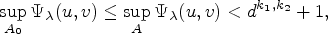
we can choose

ρ > 0

small enough such that

M_{2 ρ} \subset Ω

. Since

M

is finite, then by Lemma 2.8, there is

ε_{0} \in (0, 1)

such that for any

(u, v) \in A_{λ} ∖ (P_{δ} \cup M_{ρ})

| Ψ_{λ} (u, v) - d | \leq 2 ε_{0}

, we have

‖ V (u, v) ‖_{H_{r}}^{2} \geq ε_{0} .

(2.30)

Moreover, there is

T_{0} > 0

such that for any

(u, v) \in {\bar{M}}_{2 ρ}

‖ V (u, v) ‖_{H_{r}} \leq T_{0} .

(2.31)

Let

T := \frac{1}{2} min {1, \frac{ρ T_{2}^{2}}{4 T_{0}}} .

(2.32)

By (2.19), for the

ε_{0} > 0

, there exists

A \in {\tilde{Γ}}_{λ}^{(k_{1}, k_{2} + 1)}

such that

sup_{A ∖ P_{δ}} Ψ_{λ} (u, v) < {\tilde{d}}_{λ, δ}^{k_{1}, k_{2} + 1} + \frac{T ε_{0}}{2} = d + \frac{T ε_{0}}{2} .

(2.33)

Let

B := A ∖ M_{2 ρ}

, then

B \subset F

We claim that $γ (B) \geq (k_{1}, k_{2})$ . In view of a contradiction, suppose that $γ (B) < (k_{1}, k_{2})$ . From Definition 2.1, we know that there exists $f \in F_{(k_{1}, k_{2})} (B)$ such that $f (u, v) = (f_{1} (u, v), f_{2} (u, v)) \neq (0, 0)$ for any $(u, v) \in B$ . Take $\tilde{f} = ({\tilde{f}}_{1}, {\tilde{f}}_{2}) \in C (H, R^{k_{1} - 1} \times R^{k_{2} - 1})$ such that $\tilde{f} |_{B} = f$ by Tietze’s extension theorem. Define

\begin{aligned} F_{1} (u, v) := {\tilde{f}}_{1} (u, v) + {\tilde{f}}_{1} (σ_{2} (u, v)) - {\tilde{f}}_{1} (σ_{1} (u, v)) - {\tilde{f}}_{1} (- u, - v), \\ F_{2} (u, v) := {\tilde{f}}_{2} (u, v) + {\tilde{f}}_{2} (σ_{1} (u, v)) - {\tilde{f}}_{2} (σ_{2} (u, v)) - {\tilde{f}}_{2} (- u, - v), \end{aligned}

then

F := (F_{1}, F_{2}) \in C (H_{r}, R^{k_{1} - 1} \times R^{k_{2} - 1})

F |_{B} = 4 \tilde{f}

F_{i} (σ_{i} (u, v)) = - 4 {\tilde{f}}_{i} (u, v) = - F_{i} (u, v)

and

F_{i} (σ_{j} (u, v)) = 4 {\tilde{f}}_{i} (u, v) = F_{i} (u, v)

i \neq j

i, j = 1, 2

Define the continuous function,

g (u, v) := {\begin{cases} 1, & (u, v) \in ⋃_{n = 1}^{N} ({\bar{Ω}}_{n}^{1} \cup {\bar{Ω}}_{n}^{2}), \\ - 1, & (u, v) \in ⋃_{n = 1}^{N} ({\bar{Ω}}_{n}^{3} \cup {\bar{Ω}}_{n}^{4}), \end{cases}

and

g (σ_{1} (u, v)) = g (u, v)

g (σ_{2} (u, v)) = - g (u, v)

. Take

\tilde{g} \in C (H_{r}, R)

such that

\tilde{g} |_{Ω} = g

by Tietze’s extension theorem. Define

G (u, v) := \tilde{g} (u, v) + \tilde{g} (σ_{1} (u, v)) - \tilde{g} (σ_{2} (u, v)) - \tilde{g} (- u, - v),

then

G \in C (H_{r}, R)

G |_{Ω} = 4 \tilde{g}

G (σ_{1} (u, v)) = G (u, v)

, and

G (σ_{2} (u, v)) = - G (u, v)

. Therefore, we can define

\begin{aligned} H_{1} (u, v) := F_{1} (u, v) \in R^{k_{1} - 1}, \\ H_{2} (u, v) := (F_{2} (u, v), G (u, v)) \in R^{k_{2}}, \end{aligned}

then

H := (H_{1}, H_{2}) \in C (A, R^{k_{1} - 1} \times R^{k_{2}})

and

H \in F_{(k_{1}, k_{2} + 1)} (A)

. Since

A \in Γ_{λ}^{(k_{1}, k_{2} + 1)}

γ (A) \geq (k_{1}, k_{2} + 1)

, so there exists

(u, v) \in A

such that

H (u, v) = (0, 0)

. If

(u, v) \in B = A ∖ M_{2 ρ}

, then

F (u, v) = 4 \tilde{f} (u, v) = 4 f (u, v) \neq (0, 0),

a contradiction. Thus

(u, v) \in M_{2 ρ}

, then

G (u, v) = 4 \tilde{g} (u, v) = 4 g (u, v) \neq (0, 0),

a contradiction. Therefore,

γ (B) \geq (k_{1}, k_{2})

Since $B \subset A \subset A$ , $sup_{B} Ψ_{λ} (u, v) \leq sup_{A} Ψ_{λ} (u, v) < d^{k}$ , then we have $B \subset A_{λ}$ and $B \in {\tilde{Γ}}_{λ}^{(k_{1}, k_{2})}$ . Define $B_{0} := η (\frac{ρ}{2 T_{0}}, B)$ , then $B_{0} \subset A_{λ}$ , $B_{0} \in Γ^{(k_{1}, k_{2})}$ , $B_{0} ∖ P_{δ} \neq \emptyset$ , and $sup_{B_{0}} Ψ_{λ} (u, v) \leq sup_{B} Ψ_{λ} (u, v) < d^{k}$ by Lemmas 2.2- $(2)$ and 2.3, so $B_{0} \in {\tilde{Γ}}_{λ}^{(k_{1}, k_{2})}$ . Thus $sup_{B_{0} ∖ P_{δ}} Ψ_{λ} (u, v) \geq {\tilde{d}}_{λ, δ}^{k_{1}, k_{2}}$ by (2.19).

We claim that $η (t, (u, v)) \notin M_{ρ}$ for any $t \in (0, \frac{ρ}{2 T_{0}})$ , $(u, v) \in B$ . In view of a contradiction, if there exists $t_{0} \in (0, \frac{ρ}{2 T_{0}})$ such that $η (t_{0}, (u, v)) \in M_{ρ}$ . For $(u, v) \in B = A ∖ M_{2 ρ}$ , by the continuity of $η$ , there exists $0 \leq t_{1} < t_{2} \leq t_{0}$ satisfying $η (t_{1}, (u, v)) \in \partial M_{2 ρ}$ , $η (t_{2}, (u, v)) \in \partial M_{ρ}$ , and $η (t, (u, v)) \in M_{2 ρ} ∖ M_{ρ}$ for any $t \in (t_{1}, t_{2})$ . Then by (2.31), we have

\begin{aligned} ρ & \leq ‖ η (t_{1}, (u, v)) - η (t_{2}, (u, v)) ‖_{H_{r}} \\ = ‖ \int_{t_{1}}^{t_{2}} V (η (t, (u, v))) ‖_{H_{r}} \leq 2 T_{0} (t_{2} - t_{1}), \end{aligned}

ρ / 2 T_{0} \leq t_{2} - t_{1} \leq t_{0} - 0 < ρ / 2 T_{0}

, this yields a contradiction.

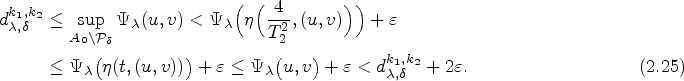
For $ε_{0} > 0$ , there exists $(u, v) \in B$ such that $η (ρ / 2 T_{0}, (u, v)) \in B_{0} ∖ P_{δ}$ satisfies

{\tilde{d}}_{λ, δ}^{k_{1}, k_{2}} \leq sup_{B_{0} ∖ P_{δ}} Ψ_{λ} (u, v) < Ψ_{λ} (η (\frac{ρ}{2 T_{0}}, (u, v))) + \frac{T ε_{0}}{2} .

Moreover,

η (t, (u, v)) \in A_{λ}

for any

t \geq 0

, then by Lemma 2.9-(4),

η (t, (u, v)) \notin P_{δ}

for any

t \in [0, \frac{ρ}{2 T_{0}}]

. Therefore,

η (t, (u, v)) \in A_{λ} ∖ (P_{δ} \cup M_{ρ}) .

(2.34)

In particular,

(u, v) \notin P_{δ}

. Moreover, by (2.33) and Lemma 2.9-

(3)

, we get

\begin{aligned} {\tilde{d}}_{λ, δ}^{k_{1}, k_{2}} & \leq sup_{B_{0} ∖ P_{δ}} Ψ_{λ} (u, v) < Ψ_{λ} (η (\frac{ρ}{2 T_{0}}, (u, v))) + \frac{T ε_{0}}{2} \\ \leq Ψ_{λ} (η (t, (u, v))) + \frac{T ε_{0}}{2} \\ \leq Ψ_{λ} (u, v) + \frac{T ε_{0}}{2} \\ < {\tilde{d}}_{λ, δ}^{k_{1}, k_{2}} + \frac{T ε_{0}}{2} + \frac{T ε_{0}}{2}, \end{aligned}

(2.35)

that is,

| Ψ_{λ} (u, v) - {\tilde{d}}_{λ, δ}^{k_{1}, k_{2}} | \leq \frac{T ε_{0}}{2} < 2 ε_{0} .

So we see from (2.30) and Lemma

2.8

that

\begin{aligned} \frac{d}{d t} Ψ_{λ} (η (t, (u, v))) & = - ⟨ \nabla Ψ_{λ} (η (t, (u, v))), V (η (t, (u, v))) ⟩_{H} \\ \leq - \frac{T_{2}^{2}}{2} ‖ V (η (t, (u, v))) ‖_{H_{r}}^{2} \leq - \frac{T_{2}^{2}}{2} ε_{0} . \end{aligned}

(2.36)

Finally, we deduce from (2.32), (2.35), and (2.36) that

\begin{aligned} {\tilde{d}}_{λ, δ}^{k_{1}, k_{2}} & < Ψ_{λ} (η (\frac{ρ}{2 T_{0}}, (u, v))) + \frac{T ε_{0}}{2} \\ \leq Ψ_{λ} (u, v) + \frac{T ε_{0}}{2} - \int_{0}^{\frac{ρ}{2 T_{0}}} \frac{T_{2}^{2}}{2} ε_{0} d t \\ < {\tilde{d}}_{λ, δ}^{k_{1}, k_{2}} + \frac{T ε_{0}}{2} + \frac{T ε_{0}}{2} - \frac{T_{2}^{2}}{2} ε_{0} \frac{ρ}{2 T_{0}} \\ = {\tilde{d}}_{λ, δ}^{k_{1}, k_{2}} + \frac{ε_{0}}{2} (2 T - \frac{T_{2}^{2} ρ}{2 T_{0}}) \leq {\tilde{d}}_{λ, δ}^{k_{1}, k_{2}}, \end{aligned}

this yields a contradiction. This completes the proof.

3. Proof of Theorem 1.2

Firstly, we give a classical result by Miranda.

Lemma 3.1
see Miranda, 1940Consider a rectangle $R = Π_{i = 1}^{s} [a_{i}, b_{i}] \subset R^{s}$ and a continuous function $I : R \to R^{s}$ , $I = (I_{1}, \dots, I_{s})$ . If $I_{i} |_{x_{i} = a_{i}} > 0 > I_{i} |_{x_{i} = b_{i}}$ holds for any $i = 1, \dots, s$ , then $I$ has a zero inside $R$ .

Using Theorem 1.1, system (2.1) has a sign-changing solution $(u_{2}, v_{2})$ for $k_{1} = k_{2} = 2$ and $δ > 0$ small enough,
$Φ_{λ} (u_{2}, v_{2}) = d_{λ, δ}^{2, 2} < d^{2, 2} + 1.$
Let
$U_{λ} := {(u, v) \in H_{r} : u, v sign-changing, Φ_{λ}^{'} (u, v) (u^{\pm}, 0) = Φ_{λ}^{'} (u, v) (0, v^{\pm}) = 0},$
then $(u_{2}, v_{2}) \in U_{λ}$ , $U_{λ} \neq \emptyset$ by Theorem 1.1, we can define
$d_{λ} := inf_{(u, v) \in U_{λ}} Φ_{λ} (u, v),$
and $d_{λ} \leq d_{λ, δ}^{2, 2} < d^{2, 2} + 1$ . $S t e p 1 :$ We claim that for any $(u, v) \in U_{λ}$ , we get
$Φ_{λ} (u, v) = sup_{t, s \in R} Φ_{λ} (t^{+} u^{+} - t^{-} u^{-}, s^{+} v^{+} - s^{-} v^{-}) .$
(3.1)
In fact, for $(u, v) \in U_{λ}$ , we have
$\begin{aligned} ‖ u^{\pm} ‖_{α}^{2} = μ | u^{\pm} |_{p + 1}^{p + 1} - | λ | \int_{R^{N}} | u^{\pm} |^{\frac{p + 1}{2}} | v |^{\frac{p + 1}{2}} d x, \\ ‖ v^{\pm} ‖_{β}^{2} = ν | v^{\pm} |_{p + 1}^{p + 1} - | λ | \int_{R^{N}} | u |^{\frac{p + 1}{2}} | v^{\pm} |^{\frac{p + 1}{2}} d x . \end{aligned}$
Then
$\begin{aligned} \int_{R^{N}} | t^{+} u^{+} - t^{-} u^{-} |^{\frac{p + 1}{2}} | s^{+} v^{+} - s^{-} v^{-} |^{\frac{p + 1}{2}} \\ = (t^{+})^{\frac{p + 1}{2}} (s^{+})^{\frac{p + 1}{2}} \int_{R^{N}} (u^{+})^{\frac{p + 1}{2}} (v^{+})^{\frac{p + 1}{2}} + (t^{+})^{\frac{p + 1}{2}} (s^{-})^{\frac{p + 1}{2}} \int_{R^{N}} (u^{+})^{\frac{p + 1}{2}} (v^{-})^{\frac{p + 1}{2}} \\ + (t^{-})^{\frac{p + 1}{2}} (s^{+})^{\frac{p + 1}{2}} \int_{R^{N}} (u^{-})^{\frac{p + 1}{2}} (v^{+})^{\frac{p + 1}{2}} + (t^{-})^{\frac{p + 1}{2}} (s^{-})^{\frac{p + 1}{2}} \int_{R^{N}} (u^{-})^{\frac{p + 1}{2}} (v^{-})^{\frac{p + 1}{2}} \\ \leq \frac{1}{2} [(t^{+})^{p + 1} \int_{R^{N}} (u^{+})^{\frac{p + 1}{2}} | v |^{\frac{p + 1}{2}} + (t^{-})^{p + 1} \int_{R^{N}} (u^{-})^{\frac{p + 1}{2}} | v |^{\frac{p + 1}{2}} \\ + (s^{+})^{p + 1} \int_{R^{N}} | u |^{\frac{p + 1}{2}} (v^{+})^{\frac{p + 1}{2}} + (s^{-})^{p + 1} \int_{R^{N}} | u |^{\frac{p + 1}{2}} (v^{-})^{\frac{p + 1}{2}}] \\ = \frac{1}{2 | λ |} [μ (t^{+})^{p + 1} | u^{+} |_{p + 1}^{p + 1} + μ (t^{-})^{p + 1} | u^{-} |_{p + 1}^{p + 1} + ν (s^{+})^{p + 1} | v^{+} |_{p + 1}^{p + 1} \\ + ν (s^{-})^{p + 1} | v^{-} |_{p + 1}^{p + 1}] \\ - \frac{1}{2 | λ |} [(t^{+})^{p + 1} ‖ u^{+} ‖_{α}^{2} + (t^{-})^{p + 1} ‖ u^{-} ‖_{α}^{2} + (s^{+})^{p + 1} ‖ v^{+} ‖_{β}^{2} + (s^{-})^{p + 1} ‖ v^{-} ‖_{β}^{2}], \end{aligned}$
so, we have
$\begin{aligned} Φ_{λ} (t^{+} u^{+} - t^{-} u^{-}, s^{+} v^{+} - s^{-} v^{-}) \\ = \frac{1}{2} [(t^{+})^{2} ‖ u^{+} ‖_{α}^{2} + (t^{-})^{2} ‖ u^{-} ‖_{α}^{2} + (s^{+})^{2} ‖ v^{+} ‖_{β}^{2} + (s^{-})^{2} ‖ v^{-} ‖_{β}^{2}] \\ - \frac{1}{p + 1} [μ (t^{+})^{p + 1} | u^{+} |_{p + 1}^{p + 1} + μ (t^{-})^{p + 1} | u^{-} |_{p + 1}^{p + 1} \\ + ν (s^{+})^{p + 1} | v^{+} |_{p + 1}^{p + 1} + ν (s^{-})^{p + 1} | v^{-} |_{p + 1}^{p + 1}] \\ + \frac{2 | λ |}{p + 1} \int_{R^{N}} | t^{+} u^{+} - t^{-} u^{-} |^{\frac{p + 1}{2}} | s^{+} v^{+} - s^{-} v^{-} |^{\frac{p + 1}{2}} \\ \leq [\frac{1}{2} (t^{+})^{2} - \frac{1}{p + 1} (t^{+})^{p + 1}] ‖ u^{+} ‖_{α}^{2} + [\frac{1}{2} (t^{-})^{2} - \frac{1}{p + 1} (t^{-})^{p + 1}] ‖ u^{-} ‖_{α}^{2} \\ + [\frac{1}{2} (s^{+})^{2} - \frac{1}{p + 1} (s^{+})^{p + 1}] ‖ v^{+} ‖_{β}^{2} + [\frac{1}{2} (s^{-})^{2} - \frac{1}{p + 1} (s^{-})^{p + 1}] ‖ v^{-} ‖_{β}^{2} \\ \leq (\frac{1}{2} - \frac{1}{p + 1}) (‖ u ‖_{α}^{2} + ‖ v ‖_{β}^{2}) = Φ_{λ} (u, v) . \end{aligned}$
Choose $(t^{+}, t^{-}, s^{+}, s^{-}) = (1, 1, 1, 1)$ , then (3.1) holds. $S t e p 2 :$ We claim that $(u_{2}, v_{2})$ is a least energy sign-changing solution of (2.1).

Choose any $(u_{0}, v_{0}) \in U_{λ}$ with $Φ_{λ} (u_{0}, v_{0}) < d^{2, 2} + 1$ , define
$\begin{aligned} A_{1} := {u \in span {u_{0}^{+}, u_{0}^{-}} : | u |_{p + 1} = 1}, \\ A_{2} := {v \in span {v_{0}^{+}, v_{0}^{-}} : | v |_{p + 1} = 1}, \end{aligned}$
then $A := A_{1} \times A_{2} \in Γ^{(2, 2)}$ . For any $(u, v) \in A$ , there exists $l_{i} \in R, i = 1, 2, 3, 4$ , such that
$u = l_{1} u_{0}^{+} + l_{2} u_{0}^{-}, v = l_{3} v_{0}^{+} + l_{4} v_{0}^{-} .$
This together with (3.1) yields
$\begin{aligned} sup_{t, s \geq 0} Φ_{λ} (t u, s v) & = sup_{t, s \geq 0} Φ_{λ} (t (l_{1} u_{0}^{+} + l_{2} u_{0}^{-}), s (l_{3} v_{0}^{+} + l_{4} v_{0}^{-})) \\ = sup_{t, s \geq 0} Φ_{λ} (t | l_{1} | u_{0}^{+} - t | l_{2} | u_{0}^{-}), s | l_{3} | v_{0}^{+} - s | l_{4} | v_{0}^{-})) \\ \leq Φ_{λ} (u_{0}, v_{0}), \end{aligned}$
that is,
$sup_{(u_{1}, u_{2}) \in A} sup_{t, s \geq 0} Φ_{λ} (t u, s v) \leq Φ_{λ} (u_{0}, v_{0}) < d^{2, 2} + 1$
then $A \in Γ_{λ}^{(2, 2)}$ and
$d_{λ, δ}^{2, 2} \leq sup_{A ∖ P_{δ}} sup_{t, s \geq 0} Φ_{λ} (t u, s v) \leq Φ_{λ} (u_{0}, v_{0}),$
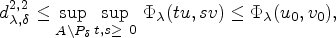
hence $d_{λ, δ}^{2, 2} \leq d_{λ}$ , so we have $d_{λ} = d_{λ, δ}^{2, 2} = Φ_{λ} (u_{2}, v_{2})$ and $(u_{2}, v_{2})$ is a least energy sign-changing solution of (2.1). $S t e p 3 :$ Since $u_{2}$ and $v_{2}$ change sign, $u_{2}$ and $v_{2}$ have at least two nodal domains. We claim that both $u_{2}$ and $v_{2}$ have exactly two nodal domains.

Suppose, in view of a contradiction, that $u_{2}$ has at least three nodal domains $O_{1}$ , $O_{2}$ , $O_{3}$ , and $u_{2} > 0$ on $O_{1} \cup O_{2}$ . Define
$f^{+} := u_{2} χ_{O_{1}}, f^{-} := u_{2} χ_{O_{2}}, g := u_{2} χ_{O_{3}},$
then $f^{\pm}, g \in H_{r}^{1} (R^{N}) ∖ {0}$ and $Φ_{λ}^{'} (u_{2}, v_{2}) (f^{\pm}, 0) = Φ_{λ}^{'} (u_{2}, v_{2}) (0, v_{2}^{\pm}) = 0$ , so
$\begin{aligned} ‖ f^{\pm} ‖_{α}^{2} = μ | f^{\pm} |_{p + 1}^{p + 1} - | λ | \int_{R^{N}} | f^{\pm} |^{\frac{p + 1}{2}} | v_{2} |^{\frac{p + 1}{2}} d x, \end{aligned}$
(3.2)

$\begin{aligned} ‖ v_{2}^{\pm} ‖_{β}^{2} = ν | v_{2}^{\pm} |_{p + 1}^{p + 1} - | λ | \int_{R^{N}} | u_{2} |^{\frac{p + 1}{2}} | v_{2}^{\pm} |^{\frac{p + 1}{2}} d x . \end{aligned}$
(3.3)
Let
$a_{1}^{p - 1} := \frac{1}{2} min {\frac{‖ f^{\pm} ‖_{α}^{2}}{μ | f^{\pm} |_{p + 1}^{p + 1}}, \frac{‖ v_{2}^{\pm} ‖_{β}^{2}}{ν | v_{2}^{\pm} |_{p + 1}^{p + 1}}},$
then $0 < a_{1} < \frac{1}{2}$ . For any $a_{2} > 1$ , we define
$\begin{aligned} I_{1}^{\pm} (t^{+}, t^{-}, s^{+}, s^{-}) & = (t^{\pm})^{2} ‖ f^{\pm} ‖_{α}^{2} - μ (t^{\pm})^{p + 1} | f^{\pm} |_{p + 1}^{p + 1} \\ + | λ | (t^{\pm})^{\frac{p + 1}{2}} \int_{R^{N}} | f^{\pm} |^{\frac{p + 1}{2}} | s^{+} v_{2}^{+} - s^{-} v_{2}^{-} |^{\frac{p + 1}{2}} d x, \\ I_{2}^{\pm} (t^{+}, t^{-}, s^{+}, s^{-}) & = (s^{\pm})^{2} ‖ v_{2}^{\pm} ‖_{β}^{2} - ν (s^{\pm})^{p + 1} | v_{2}^{\pm} |_{p + 1}^{p + 1} \\ + | λ | (s^{\pm})^{\frac{p + 1}{2}} \int_{R^{N}} | t^{+} f^{+} - t^{-} f^{-} |^{\frac{p + 1}{2}} | v_{2}^{\pm} |^{\frac{p + 1}{2}} d x . \end{aligned}$
Then for any $(t^{+}, t^{-}, s^{+}, s^{-}) \in [a_{1}, a_{2}]^{4}$ , by (3.2) and (3.3), we get
$\begin{aligned} I_{1}^{\pm} |_{t^{\pm} = a_{1}} & \geq a_{1}^{2} ‖ f^{\pm} ‖_{α}^{2} - μ a_{1}^{p + 1} | f^{\pm} |_{p + 1}^{p + 1} \geq \frac{1}{2} a_{1}^{2} ‖ f^{\pm} ‖_{α}^{2} > 0, \end{aligned}$
(3.4)

$\begin{aligned} I_{2}^{\pm} |_{s^{\pm} = a_{1}} & \geq a_{1}^{2} ‖ v_{2}^{\pm} ‖_{β}^{2} - ν a_{1}^{p + 1} | v_{2}^{\pm} |_{p + 1}^{p + 1} \geq \frac{1}{2} a_{1}^{2} ‖ v_{2}^{\pm} ‖_{β}^{2} > 0, \end{aligned}$
(3.5)

$\begin{aligned} I_{1}^{\pm} |_{t^{\pm} = a_{2}} & = a_{2}^{2} ‖ f^{\pm} ‖_{α}^{2} - μ a_{2}^{p + 1} | f^{\pm} |_{p + 1}^{p + 1} \\ + | λ | a_{2}^{\frac{p + 1}{2}} \int_{R^{N}} | f^{\pm} |^{\frac{p + 1}{2}} ((s^{+})^{\frac{p + 1}{2}} (v_{2}^{+})^{\frac{p + 1}{2}} + (s^{-})^{\frac{p + 1}{2}} (v_{2}^{-})^{\frac{p + 1}{2}}) d x \\ \leq a_{2}^{2} ‖ f^{\pm} ‖_{α}^{2} - μ a_{2}^{p + 1} | f^{\pm} |_{p + 1}^{p + 1} + | λ | a_{2}^{p + 1} \int_{R^{N}} | f^{\pm} |^{\frac{p + 1}{2}} | v_{2} |^{\frac{p + 1}{2}} \\ = (a_{2}^{2} - a_{2}^{p + 1}) ‖ f^{\pm} ‖_{α}^{2} < 0, \end{aligned}$
(3.6)

$\begin{aligned} I_{2}^{\pm} |_{s^{\pm} = a_{2}} & \leq (a_{2}^{2} - a_{2}^{p + 1}) ‖ v_{2}^{\pm} ‖_{β}^{2} < 0. \end{aligned}$
(3.7)
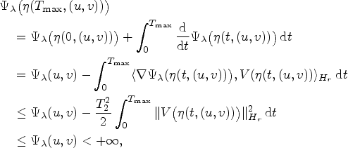
Moreover, from (3.4) to (3.7) and Lemma 3.1, we see that there exists $(t_{0}^{+}, t_{0}^{-}, s_{0}^{+}, s_{0}^{-}) \in [a_{1}, a_{2}]^{4}$ satisfying $0 < t_{0}^{\pm}, s_{0}^{\pm} \leq 1$ and $I_{1}^{\pm} (t_{0}^{+}, t_{0}^{-}, s_{0}^{+}, s_{0}^{-}) = I_{2}^{\pm} (t_{0}^{+}, t_{0}^{-}, s_{0}^{+}, s_{0}^{-}) = 0$ . Therefore, $(t_{0}^{+} f^{+} - t_{0}^{-} f^{-}, s_{0}^{+} v_{2}^{+} - s_{0}^{-} v_{2}^{-}) \in U_{λ}$ and
$\begin{aligned} d_{λ, δ}^{2, 2} & \leq Φ_{λ} (t_{0}^{+} f^{+} - t_{0}^{-} f^{-}, s_{0}^{+} v_{2}^{+} - s_{0}^{-} v_{2}^{-}) \\ = (\frac{1}{2} - \frac{1}{p + 1}) ((t_{0}^{+})^{2} ‖ f^{+} ‖_{α}^{2} + (t_{0}^{-})^{2} ‖ f^{-} ‖_{α}^{2} + (s_{0}^{+})^{2} ‖ v_{2}^{+} ‖_{β}^{2} + (s_{0}^{-})^{2} ‖ v_{2}^{-} ‖_{β}^{2}) \\ \leq (\frac{1}{2} - \frac{1}{p + 1}) (‖ f^{+} ‖_{α}^{2} + ‖ f^{-} ‖_{α}^{2} + ‖ v_{2}^{+} ‖_{β}^{2} + ‖ v_{2}^{-} ‖_{β}^{2}) \\ < (\frac{1}{2} - \frac{1}{p + 1}) (‖ u_{2} ‖_{α}^{2} + ‖ v_{2} ‖_{β}^{2}) = Φ_{λ} (u_{2}, v_{2}) = d_{λ, δ}^{2, 2}, \end{aligned}$
this yields a contradiction. Hence, $u_{2}$ has exactly two nodal domains. Similarly, $v_{2}$ has exactly two nodal domains. This completes the proof.
4. The Proof of Theorem 1.3

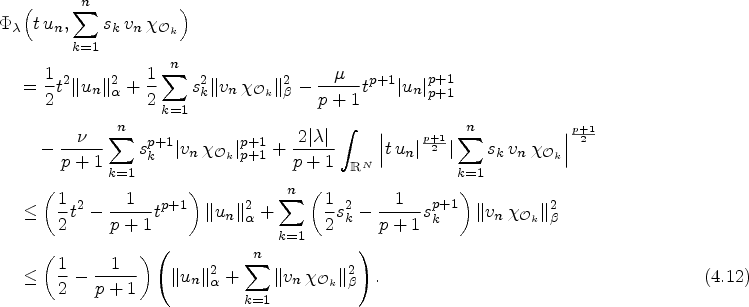
In this section, we obtain infinitely many radially symmetric semi-nodal solutions $(u, v)$ such that $u$ is positive, $v$ is sign-changing. We use the same notations as in Section 2 for convenience. Define the $C^{1}$ functional

\begin{aligned} Φ_{λ} (u, v) & := \frac{1}{2} (‖ u ‖_{α}^{2} + ‖ v ‖_{β}^{2}) - \frac{1}{p + 1} (μ | u^{+} |_{p + 1}^{p + 1} + ν | v |_{q + 1}^{q + 1}) \\ + \frac{2 | λ |}{p + 1} \int_{R^{N}} | u |^{\frac{p + 1}{2}} | v |^{\frac{p + 1}{2}} d x, \end{aligned}

where

(u, v) \in \tilde{H} := {(u, v) \in H_{r} : u^{+} \neq 0, v \neq 0}

\begin{aligned} A & := {(u, v) \in H_{r} : | u^{+} |_{p + 1} = 1, | v |_{p + 1} = 1}, \\ A^{*} & := {(u, v) \in H_{r} : | u^{+} |_{p + 1} > \frac{1}{2}, | v |_{p + 1} > \frac{1}{2}}, \\ A_{λ}^{*} & := {(u, v) \in A^{*} : \frac{4 | λ |}{(p + 1)^{2}} (\int_{R^{N}} | u |^{\frac{p + 1}{2}} | v |^{\frac{p + 1}{2}} d x)^{2} < μ ν | u^{+} |_{p + 1}^{p + 1} | v |_{p + 1}^{p + 1}}, \\ A_{λ}^{* *} & := {(u, v) \in A^{*} : \frac{4 | λ |}{(p + 1)^{2}} (\int_{R^{N}} | u |^{\frac{p + 1}{2}} | v |^{\frac{p + 1}{2}} d x)^{2} < μ ν}, \\ A_{λ} & := A \cap A_{λ}^{*} = A \cap A_{λ}^{* *} . \end{aligned}

Lemma 4.1
If for any $u, v \in H_{r}^{1} (R^{N}), u \neq 0, v \neq 0$ , such that
$\frac{4 | λ |^{2}}{(p + 1)^{2}} (\int_{R^{N}} | u |^{\frac{p + 1}{2}} | v |^{\frac{p + 1}{2}} d x)^{2} \geq μ ν | u^{+} |_{p + 1}^{p + 1} | v |_{p + 1}^{p + 1},$
then
$sup_{t, s \geq 0} Φ_{λ} (t u, s v) = + \infty .$

Proof.
It is easy to prove that Lemma 4.1 by trivial modifications.

As in Section 2, for any $(u, v) \in A$ , we define
$sup_{t, s \geq 0} Φ_{λ} (t u, s v) = Φ_{λ} (t_{u, v, λ} u, s_{u, v, λ} v) =: Ψ_{λ} (u, v) .$
(4.1)
For any $(u, v) \in A_{λ}^{}$ , we consider the following linear problem:
${\begin{cases} - Δ φ + α φ + t_{u, v, λ}^{\frac{p - 3}{2}} s_{u, v, λ}^{\frac{p + 1}{2}} | λ | | u |^{\frac{p - 3}{2}} φ | v |^{\frac{p + 1}{2}} = μ t_{u, v, λ}^{p - 1} (u^{+})^{p}, \\ - Δ ψ + β ψ + t_{u, v, λ}^{\frac{p + 1}{2}} s_{u, v, λ}^{\frac{p - 3}{2}} | λ | | u |^{\frac{p + 1}{2}} | v |^{\frac{p - 3}{2}} ψ = ν s_{u, v, λ}^{p - 1} | v |^{p - 1} v, \\ φ (x) \to 0, ψ (x) \to 0, as | x | \to \infty, \end{cases}$
(4.2)
then (4.2) has unique solution $(φ, ψ)$ . Define
$a := \frac{1}{\int_{R^{N}} (u^{+})^{p} φ d x} > 0, b := \frac{1}{\int_{R^{N}} | v |^{p - 1} v ψ d x} > 0.$
Then $(\tilde{φ}, \tilde{ψ}) := (a φ, b ψ)$ is the unique solution of the following problem:
${\begin{cases} - Δ \tilde{φ} + α \tilde{φ} + t_{u, v, λ}^{\frac{p - 3}{2}} s_{u, v, λ}^{\frac{p + 1}{2}} | λ | | u |^{\frac{p - 3}{2}} \tilde{φ} | v |^{\frac{p + 1}{2}} = a μ t_{u, v, λ}^{p - 1} (u^{+})^{p}, \\ - Δ \tilde{ψ} + β \tilde{ψ} + t_{u, v, λ}^{\frac{p + 1}{2}} s_{u, v, λ}^{\frac{p - 3}{2}} | λ | | u |^{\frac{p + 1}{2}} | v |^{\frac{p - 3}{2}} \tilde{ψ} = b ν s_{u, v, λ}^{p - 1} | v |^{p - 1} v, \\ \int_{R^{N}} (u^{+})^{p} \tilde{φ} d x = \int_{R^{N}} | v |^{p - 1} v \tilde{ψ} d x = 1, \\ \tilde{φ} (x) \to 0, \tilde{ψ} (x) \to 0, as\, | x | \to \infty . \end{cases}$
(4.3)
We can now also define the operator
$\begin{aligned} K : A_{λ}^{} \to H_{r}; (u, v) \mapsto (\tilde{φ}, \tilde{ψ}), \\ K (σ_{2} (u, v)) = σ_{2} (K (u, v)) . \end{aligned}$
(4.4)
Then by similar proofs as in Lemmas 2.5 and 2.6, we have that $K \in C^{1} (A_{λ}^{}, H_{r})$ and $K$ satisfies Palais-Smale type condition. Define the map
$V : A_{λ}^{} \to H_{r}; (u, v) \mapsto (u, v) - K (u, v) .$
Consider the class of sets
$F = {A \in A : A \,is a closed set and σ_{2} (u, v) \in A, \forall (u, v) \in A},$
(4.5)
for each $A \in F$ and $k_{2} \geq 2$ , the class of functions
$F_{(1, k_{2})} (A) = {f : A \to R^{k_{2} - 1} : f continuous, f (σ_{2} (u, v)) = - f (u, v)} .$
(4.6)
To obtain semi-nodal solutions, we should also define cones of positive functions, that is,
$\begin{aligned} P_{2} := {(u, v) \in H : v \geq 0}, P = P_{2} \cup - P_{2}, \\ {dist}_{p + 1} ((u, v), P) := min {{dist}_{p + 1} (v, P_{2}), {dist}_{p + 1} (v, - P_{2})}, \end{aligned}$
(4.7)
thus, $v$ is sign-changing if ${dist}_{p + 1} ((u, v), P) > 0$ .

Under the new definitions (4.4)–(4.6), we define vector genus, slightly different from Definition 2.1.
Definition 4.1
Let $A \in F$ and take any $k_{2} \in N$ with $k_{2} \geq 2$ . We say that $γ (A) \geq (1, k_{2})$ if for every $f \in F_{(1, k_{2})} (A)$ there exists $(u, v) \in A$ such that $f (u, v) = 0$ . We denote
$Γ^{(1, k_{2})} := {A \in F : γ (A) \geq (1, k_{2})} .$

Lemma 4.2
(1)
Take $A := A_{1} \times A_{2} \subset A$ and let $η : S^{k_{2} - 1} \to A_{2}$ be a homeomorphism such that $η (- x) = - η (x)$ for every $x \in S^{k_{2} - 1}$ . Then $A \in Γ^{(1, k_{2})}$ .
(2)
We have $\bar{η (A)} \in Γ^{(1, k_{2})}$ whenever $A \in Γ^{(1, k_{2})}$ and a continuous map $η : A \to A$ such that $η \circ σ_{2} = σ_{2} \circ η .$

Proof.
(1)
For every $f \in F_{(1, k_{2})} (A)$ and $u \in A_{1}$ , we define a map
$h : S^{k_{2} - 1} \to R^{k_{2} - 1}; h (x) := f (u, η (x)),$
then by (4.6), it is easy to see that $h$ is continuous and
$h (- x) = f (u, η (- x)) = f (u, - η (x)) = - f (u, η (x)) = - h (x) .$
Then Borsuk-Ulam theorem yields $x_{0} \in S^{k_{2} - 1}$ such that $h (x_{0}) = f (u, η (x_{0})) = 0$ . By Definition $4.1$ , we have $A \in Γ^{(1, k_{2})}$ .
(2)
Fix any $f \in F_{(1, k_{2})} (\bar{η (A)})$ , then by (4.6), we have $f \circ η \in F_{(1, k_{2})} (A)$ . Since $A \in Γ^{(1, k_{2})}$ , there exists $(u_{0}, v_{0}) \in A$ such that $f \circ η (u_{0}, v_{0}) = 0$ . Then by $η (u_{0}, v_{0}) \in \bar{η (A)}$ , we have $γ (\bar{η (A)}) \geq (1, k_{2})$ , that is, $\bar{η (A)} \in Γ^{(1, k_{2})}$ . This completes the proof.

Lemma 4.3
Assume $k_{2} \geq 2$ . Then for any $0 < δ < 2^{- \frac{1}{p + 1}}$ and $A \in Γ^{(1, k_{2})}$ , we have $A ∖ P_{δ} \neq \emptyset$ .
Proof.
For any $A \in Γ^{(1, k_{2})}$ , define $f$ by
$f (u, v) = (\int_{R^{N}} | v |^{p} v d x, 0, \dots, 0),$
then $f \in F_{(1, k_{2})} (A)$ , so by Definition $4.1$ , there exists $(u_{0}, v_{0}) \in A$ such that $f (u_{0}, v_{0}) = 0.$ We deduce from $A \in A$ that $\int_{R^{N}} (v_{0}^{+})^{p + 1} d x = \int_{R^{N}} (v_{0}^{-})^{p + 1} d x = \frac{1}{2}$ . Therefore, ${dist}_{p + 1} ((u_{0}, v_{0}), P) = 2^{- \frac{1}{p + 1}}$ and so $(u_{0}, v_{0}) \in A ∖ P_{δ}$ for any $δ < 2^{- \frac{1}{p + 1}}$ .This completes the proof.

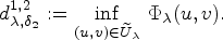
Fixed any $k_{1}, k_{2} \geq 2$ , similarly as in Section 2, take nonempty open subsets $Ω_{1}, Ω_{2} \subset R^{N}$ with $Ω_{1} \cap Ω_{2} = \emptyset$ , ${U_{i} : 1 \leq i \leq k_{1}}$ and ${V_{i} : 1 \leq i \leq k_{2}}$ as in (2.17) and (2.18). We define
$A_{1} := {\frac{U_{1}}{| U_{1} |_{p + 1}}}, A_{2} := {v \in span {V_{1}, \dots, V_{k_{2}}} : | v |_{p + 1} = 1} .$
By Lemma 4.2- $(1)$ , $A := A_{1} \times A_{2} \in Γ^{(1, k)}$ . Similarly, for any $λ < 0$ ,
$sup_{A} sup_{t, s \geq 0} Φ_{λ} (t u, s v) \leq d^{1, k_{2}} .$
Then we can define
$Γ_{λ}^{(1, k_{2})} := {A \in Γ^{(1, k_{2})} : sup_{A} sup_{t, s \geq 0} Φ_{λ} (t u, s v) < d^{1, k_{2}} + 1} .$
For any $k_{2} \geq 2$ and $0 < δ < 2^{- \frac{1}{p + 1}}$ , we define a sequence of minimax energy level,
$d_{λ, δ}^{1, k_{2}} := inf_{A \in Γ_{λ}^{(1, k_{2})}} sup_{A ∖ P_{δ}} sup_{t, s \geq 0} Φ_{λ} (t u, s v) .$
It is easy to see that
$d_{λ, δ}^{1, k_{2}} < d^{1, k_{2}}, for \,any 0 < δ < 2^{- \frac{1}{p + 1}} and k_{2} \geq 2.$
Lemmas 2.7 and 2.8 also hold in the case of the current Section 4.
Lemma 4.4
There exists a unique global solution $η : R^{+} \times A_{λ} \to H_{r}$ for the initial value problem
${\begin{cases} \frac{d}{d t} η (t, (u, v)) = - V (η (t, (u, v))), \\ η (0, (u, v)) = (u, v) \in A_{λ} . \end{cases}$
(4.8)
Moreover, $(1),(3),(4)$ of Lemma 2.9 hold and (1)
For any $t > 0$ , $(u, v) \in A_{λ}$ , $η (t, σ_{2} (u, v)) = σ_{2} (η (t, (u, v)))$ .

Proof.
From the above discussion, we see that $V \in C^{1} (A_{λ}^{}, H_{r})$ . As $A_{λ} \subset A_{λ}^{}$ , we get that $V \in C^{1} (A_{λ}, H_{r})$ , then there exists a solution $η : [0, T_{max}) \times A_{λ} \to H_{r}$ , where $T_{max}$ is the maximal time such that (4.8) has s solution $η \in A_{λ}^{*}$ .

For any $(u, v) \in A_{λ}$ and $t \in (0, T_{max})$ , there holds
$\begin{aligned} \frac{d}{d t} \int_{R^{N}} (η_{1}^{+} (t, (u, v)))^{p + 1} d x \\ = - (p + 1) \int_{R^{N}} (η_{1}^{+} (t, (u, v)))^{p} V (η_{1}^{+} (t, (u, v))) d x \\ = - (p + 1) \int_{R^{N}} (η_{1}^{+} (t, (u, v)))^{p} [η_{1}^{+} (t, (u, v)) - K_{1} (η^{+} (t, (u, v)))] d x \\ = (p + 1) - (p + 1) \int_{R^{N}} (η_{1}^{+} (t, (u, v)))^{p + 1} d x, \end{aligned}$
so we have
$\frac{d}{d t} [e^{(p + 1) t} (\int_{R^{N}} (η_{1}^{+} (t, (u, v)))^{p + 1} d x - 1)] = 0.$
Since $\int_{R^{N}} (η_{1}^{+} (0, (u, v)))^{p + 1} d x = \int_{R^{N}} (u^{+})^{p + 1} d x = 1$ , then for any $t \in [0, T_{max})$ ,
$\int_{R^{N}} (η_{1}^{+} (t, (u, v)))^{p + 1} d x \equiv 1.$
The rest of the proof is the same as Lemma 2.9. This completes the proof.
Proof The proof of Theorem 1.3.

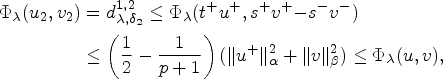
$S t e p 1 :$ Observe that from Lemma 2.10, for any $k_{2} \geq 2$ , $0 < δ < δ_{0}$ small, there exists $(u_{0}, v_{0}) \in A_{λ}$ such that

Ψ_{λ} (u_{0}, v_{0}) = d_{λ, δ}^{1, k_{2}}, V (u_{0}, v_{0}) = 0 and {dist}_{p + 1} ((u_{0}, v_{0}), P) \geq δ .

We conclude that

v_{0}

is sign-changing and

(u_{0}, v_{0}) = K (u_{0}, v_{0}) = ({\tilde{φ}}_{0}, {\tilde{ψ}}_{0})

. It follows from (4.3) that

(u_{0}, v_{0})

satisfies:

{\begin{cases} - Δ u_{0} + α u_{0} = a μ t_{u, v, λ}^{p - 1} (u_{0}^{+})^{p} + t_{u_{0}, v_{0}, λ}^{\frac{p - 3}{2}} s_{u_{0}, v_{0}, λ}^{\frac{p + 1}{2}} λ | u_{0} |^{\frac{p - 3}{2}} u_{0} | v_{0} |^{\frac{p + 1}{2}}, \\ - Δ v_{0} + β v_{0} = b ν s_{u_{0}, v_{0}, λ}^{p - 1} | v_{0} |^{p - 1} v_{0} + t_{u_{0}, v_{0}, λ}^{\frac{p + 1}{2}} s_{u_{0}, v_{0}, λ}^{\frac{p - 3}{2}} λ | u_{0} |^{\frac{p + 1}{2}} | v_{0} |^{\frac{p - 3}{2}} v_{0}, \\ u_{0} (x) \to 0, v_{0} (x) \to 0, as\, | x | \to \infty . \end{cases}

(4.9)

On the other hand,

| u_{0}^{+} |_{p + 1} = | v_{0} |_{p + 1} = 1

, we have

a = b = 1

. Moreover, (4.9) yields

‖ u_{0}^{-} ‖_{α}^{2} = t_{u_{0}, v_{0}, λ}^{\frac{p - 3}{2}} s_{u_{0}, v_{0}, λ}^{\frac{p + 1}{2}} λ \int_{R^{N}} | u_{0} |^{\frac{p - 3}{2}} (u_{0}^{-})^{2} | v_{0} |^{\frac{p + 1}{2}},

then

‖ u_{0}^{-} ‖_{α}^{2} = 0

, so

u_{0} \geq 0

. By the strong maximum principle,

u_{0} > 0

. Hence we have that

(t_{u_{0}, v_{0}, λ} u_{0}, s_{u_{0}, v_{0}, λ} v_{0})

is a semi-nodal solution of

(1.1)

with

t_{u_{0}, v_{0}, λ} u_{0}

positive,

s_{u_{0}, v_{0}, λ} v_{0}

sign-changing and

Φ_{λ} (t_{u_{0}, v_{0}, λ} u_{0}, s_{u_{0}, v_{0}, λ} v_{0}) = Ψ_{λ} (u_{0}, v_{0}) = d_{λ, δ}^{1, k_{2}} \leq d^{1, k_{2}} .

S t e p 2 :

We claim that (2.1) has infinitely many radially symmetric semi-nodal solutions. Suppose, in view of a contradiction, that there exists

k_{n} \to \infty

δ_{n} \in (0, 2^{- \frac{1}{p + 1}}]

and

M > 0

such that

d_{λ, δ}^{1, k_{n}} \leq M, \forall n \in N .

By similar arguments as in the proof of Theorem

1.4

, we get a contradiction. Thus, (2.1) has infinitely many radially symmetric semi-nodal solutions

{(u_{n}, v_{n})}_{n \geq 2}

with

u_{n}

positive and

v_{n}

sign-changing.

S t e p 3 :

We claim that

v_{n}

has at most

n

nodal domains. Suppose, in view of a contradiction, that

v_{n}

has at least

n + 1

nodal domains

O_{k}

1 \leq k \leq n + 1

, then

v_{n} χ_{O_{k}} \in H_{r}^{1} (R^{N})

and

Φ_{λ}^{'} (u_{n}, v_{n}) (u_{n}, 0) = Φ_{λ}^{'} (u_{n}, v_{n}) (0, v_{n} χ_{O_{k}}) = 0,

and so

\begin{aligned} ‖ u_{n} ‖_{α}^{2} = μ | u_{n} |_{p + 1}^{p + 1} - | λ | \int_{R^{N}} | u_{n} |^{\frac{p + 1}{2}} | v_{n} |^{\frac{p + 1}{2}} d x, \end{aligned}

(4.10)

\begin{aligned} ‖ v_{n} χ_{O_{k}} ‖_{β}^{2} = ν | v_{n} χ_{O_{k}} |_{p + 1}^{p + 1} - | λ | \int_{R^{N}} | u_{n} |^{\frac{p + 1}{2}} | v_{n} χ_{O_{k}} |^{\frac{p + 1}{2}} d x . \end{aligned}

(4.11)

Then by (4.10) and (4.11), for

t, s_{1}, \dots, s_{n} \geq 0

u_{n} \geq 0

, we have

\begin{aligned} d \int_{R^{N}} | t u_{n} |^{\frac{p + 1}{2}} | \sum_{k = 1}^{n} s_{k} v_{n} χ_{O_{k}} |^{\frac{p + 1}{2}} \\ \leq \frac{t^{p + 1}}{2} \int_{R^{N}} | u_{n} |^{\frac{p + 1}{2}} | v_{n} |^{\frac{p + 1}{2}} d x + \frac{1}{2} \sum_{k = 1}^{n} s_{k}^{p + 1} \int_{R^{N}} | u_{n} |^{\frac{p + 1}{2}} | v_{n} χ_{O_{k}} |^{\frac{p + 1}{2}} d x \\ = \frac{1}{2 | λ |} (μ t^{p + 1} | u_{n} |_{p + 1}^{p + 1} + ν \sum_{k = 1}^{n} s_{k}^{p + 1} | v_{n} χ_{O_{k}} |_{p + 1}^{p + 1}) \\ - \frac{1}{2 | λ |} (t^{p + 1} ‖ u_{n} ‖_{α}^{2} + \sum_{k = 1}^{n} s_{k}^{p + 1} ‖ v_{n} χ_{O_{k}} ‖_{β}^{2}), \end{aligned}

so, we have

\begin{aligned} Φ_{λ} (t u_{n}, \sum_{k = 1}^{n} s_{k} v_{n} χ_{O_{k}}) \\ = \frac{1}{2} t^{2} ‖ u_{n} ‖_{α}^{2} + \frac{1}{2} \sum_{k = 1}^{n} s_{k}^{2} ‖ v_{n} χ_{O_{k}} ‖_{β}^{2} - \frac{μ}{p + 1} t^{p + 1} | u_{n} |_{p + 1}^{p + 1} \\ - \frac{ν}{p + 1} \sum_{k = 1}^{n} s_{k}^{p + 1} | v_{n} χ_{O_{k}} |_{p + 1}^{p + 1} + \frac{2 | λ |}{p + 1} \int_{R^{N}} | t u_{n} |^{\frac{p + 1}{2}} | \sum_{k = 1}^{n} s_{k} v_{n} χ_{O_{k}} |^{\frac{p + 1}{2}} \\ \leq (\frac{1}{2} t^{2} - \frac{1}{p + 1} t^{p + 1}) ‖ u_{n} ‖_{α}^{2} + \sum_{k = 1}^{n} (\frac{1}{2} s_{k}^{2} - \frac{1}{p + 1} s_{k}^{p + 1}) ‖ v_{n} χ_{O_{k}} ‖_{β}^{2} \\ \leq (\frac{1}{2} - \frac{1}{p + 1}) (‖ u_{n} ‖_{α}^{2} + \sum_{k = 1}^{n} ‖ v_{n} χ_{O_{k}} ‖_{β}^{2}) . \end{aligned}

(4.12)

We define

A_{1} := {\frac{u_{n}}{| u_{n} |_{p + 1}}}, A_{2} := {v \in span {v_{n} χ_{O_{1}}, \dots, v_{n} χ_{O_{n}}} : | v |_{p + 1} = 1} .

By Lemma 4.2-

(1)

A := A_{1} \times A_{2} \in Γ^{(1, n)}

. Again by using (4.1) we obtain

\begin{aligned} sup_{A} sup_{t, s \geq 0} Φ_{λ} (t u, s v) & \leq (\frac{1}{2} - \frac{1}{p + 1}) (‖ u_{n} ‖_{α}^{2} + \sum_{k = 1}^{n} ‖ v_{n} χ_{O_{k}} ‖_{β}^{2}) \\ < (\frac{1}{2} - \frac{1}{p + 1}) (‖ u_{n} ‖_{α}^{2} + ‖ v_{n} ‖_{β}^{2}) \\ = Φ_{λ} (u_{n}, v_{n}) = d_{λ, δ_{n}}^{1, n} \leq d^{1, n}, \end{aligned}

thus

A \in Γ_{λ}^{(1, n)}

, then

\begin{aligned} d_{λ, δ_{n}}^{1, n} & \leq sup_{A ∖ P_{δ}} sup_{t, s \geq 0} Φ_{λ} (t u, s v) \\ \leq (\frac{1}{2} - \frac{1}{p + 1}) (‖ u_{n} ‖_{α}^{2} + \sum_{k = 1}^{n} ‖ v_{n} χ_{O_{k}} ‖_{β}^{2}) < Φ_{λ} (u_{n}, v_{n}) . \end{aligned}

Thus it implies a contradiction and, therefore,

v_{n}

has at most

n

nodal domains.

S t e p 4 :

We claim that

(u_{2}, v_{2})

is a least energy sign-changing solution of (2.1) with

u_{2}

positive and

v_{2}

sign-changing.

Define

{\tilde{U}}_{λ} := {(u, v) \in H_{r} : u \geq 0, v sign-changing, Φ_{λ}^{'} (u, v) (u, 0) = Φ_{λ}^{'} (u, v) (0, v^{\pm}) = 0} .

Similarly as Step

2

in Theorem

1.2

, we have

d_{λ, δ_{2}}^{1, 2} := inf_{(u, v) \in {\tilde{U}}_{λ}} Φ_{λ} (u, v) .

For any semi-nodal solution

(u, v)

of (2.1) with

v

sign-changing, by similar arguments as in Theorem

1.2

, there exist

t^{\pm}, s^{\pm} \in (0, 1]

satisfying

(t^{+} u^{+}, s^{+} v^{+} - s^{-} v^{-}) \in {\tilde{U}}_{λ},

and so

\begin{aligned} Φ_{λ} (u_{2}, v_{2}) & = d_{λ, δ_{2}}^{1, 2} \leq Φ_{λ} (t^{+} u^{+}, s^{+} v^{+} - s^{-} v^{-}) \\ \leq (\frac{1}{2} - \frac{1}{p + 1}) (‖ u^{+} ‖_{α}^{2} + ‖ v ‖_{β}^{2}) \leq Φ_{λ} (u, v), \end{aligned}

then

(u_{2}, v_{2})

is a least energy sign-changing solution. We complete the proof.

5. Proof of Theorems 1.4 and 1.5

We consider the case when $Ω \subset R^{N}$ is a smooth bounded domain,

{\begin{cases} - Δ u + α u = μ | u |^{p - 1} u + λ | u |^{\frac{p - 3}{2}} u | v |^{\frac{p + 1}{2}}, x \in Ω, \\ - Δ v + β v = ν | v |^{p - 1} v + λ | u |^{\frac{p + 1}{2}} | v |^{\frac{p - 3}{2}} v, x \in Ω, \\ u = v = 0 x \in \partial Ω . \end{cases}

(5.1)

Since the embedding

H_{0}^{1} (Ω) ↪ L^{p + 1} (Ω)

is compact, it is easy to see that after trivial modifications, all arguments in Sections 2–4 hold for system (5.1) by replacing

H_{r}^{1} (R^{N}), H_{r}

with

H_{0}^{1} (Ω), H

, respectively. Here we give a quiet different proof from those in Theorems

1.1

1.2

, and

1.3

, but cannot be used in

R^{N}

Proof The proof of Theorem 1.4.

It is enough to check that

lim_{k_{1} \to \infty} inf_{δ \in (0, 2^{- \frac{1}{p + 1}})} d_{λ, δ}^{k_{1}, k_{2}} = + \infty .

(5.2)

In fact, if (5.2) holds and so (5.1) has infinitely many sign-changing solutions

(u_{n}, v_{n})

satisfying

Φ_{λ} (u_{n}, v_{n}) \to + \infty

n \to \infty

and

u_{n}, v_{n} \in L^{\infty} (R^{N})

by standard elliptic regularity theory. Observe that

\begin{aligned} Φ_{λ} (u_{n}, v_{n}) & = (\frac{1}{2} - \frac{1}{p + 1}) (μ | u_{n} |_{p + 1}^{p + 1} + ν | v_{n} |_{p + 1}^{p + 1}) \\ - \frac{p - 1}{p + 1} | λ | \int_{Ω} | u_{n} |^{\frac{p + 1}{2}} | v_{n} |^{\frac{p + 1}{2}} d x \\ \leq (\frac{1}{2} - \frac{1}{p + 1}) (μ | Ω | | u_{n} |_{L^{\infty}}^{p + 1} + ν | Ω | | v_{n} |_{L^{\infty}}^{p + 1}), \end{aligned}

then we have

‖ u_{n} ‖_{L^{\infty} (Ω)} + ‖ v_{n} ‖_{L^{\infty} (Ω)} \to + \infty, as n \to \infty .

Now, we prove that (5.2). Suppose, in view of a contradiction, that there exists

k_{1, n} \to \infty

δ_{n} \in (0, 2^{- \frac{1}{p + 1}}]

and

M > 0

such that

d_{λ, δ}^{k_{1, n}, k_{2}} \leq M, for any n \in N .

By (2.19), there exists

A_{n} \in Γ_{λ}^{(k_{1, n}, k_{2})}

such that

sup_{A_{n} ∖ P_{δ_{n}}} sup_{t, s \geq 0} Φ_{λ} (t u, s v) \leq M + 1, for any n \in N .

Let

{e_{k}}_{k} \subset H_{0}^{1} (Ω)

be the eigenfunctions of

(- Δ, H_{0}^{1} (Ω))

and

{ξ_{k}}_{k}

be the corresponding eigenvalues with

ξ_{k} \to + \infty

k \to + \infty

. Define

h_{n} = (h_{1, n}, h_{2, n}) : A_{n} \to R^{k_{1, n} - 1} \times R^{k_{2} - 1},

\begin{aligned} h_{1, n} : A_{n} \to R^{k_{1, n} - 1}; (u, v) \mapsto (\int_{Ω} e_{1} u d x, \dots, \int_{Ω} e_{k_{1, n} - 2} u d x, \int_{Ω} | u |^{p} u d x), \\ h_{2, n} : A_{n} \to R^{k_{2} - 1}; (u, v) \mapsto (\int_{Ω} e_{1} v d x, \dots, \int_{Ω} e_{k_{2} - 2} v d x, \int_{Ω} | v |^{p} v d x), \end{aligned}

we have

h_{n} \in F_{(k_{1, n}, k_{2})} (A_{n})

, then by Definition

2.1

, there exists

(u_{n}, v_{n}) \in A_{n}

such that

h_{n} (u_{n}, v_{n}) = 0

. By Lemma 2.3,

(u_{n}, v_{n}) \in A_{n} ∖ P_{δ_{n}}

, so

sup_{t, s \geq 0} Φ_{λ} (t u_{n}, s v_{n}) \leq M + 1, for any n \in N .

Observe that from

h_{n} (u_{n}, v_{n}) = 0

, we deduce that

u_{n} \in span {e_{1}, \dots, e_{k_{1, n} - 2}}^{⊥}

and so

\frac{\int_{Ω} | \nabla u_{n} |^{2} d x}{\int_{Ω} | u_{n} |^{2} d x} \geq ξ_{k_{1, n} - 1} .

(5.3)

Moreover,

(\frac{1}{2} - \frac{1}{p + 1}) t_{u, v, λ}^{2} ‖ u_{n} ‖_{α}^{2} \leq sup_{t, s \geq 0} Φ_{λ} (t u_{n}, s v_{n}) \leq M + 1,

we have that

{u_{n}}_{n \geq 1}

are uniformly bounded in

H_{0}^{1} (Ω)

. Then, up to a subsequence, we get

\begin{aligned} u_{n} ⇀ u_{0} weakly in H_{0}^{1} (Ω), \\ u_{n} \to u_{0}, strongly in L^{p + 1} (Ω) \cap L^{2} (Ω) . \end{aligned}

u_{n} \in A_{n} ∖ P_{δ} \subset A

| u_{n} |_{p + 1} = 1

, there holds

| u_{0} |_{p + 1} = 1

. But from (5.3), we get

\int_{Ω} | u_{n} |^{2} d x \to 0

, then

u_{0} = 0

, a contradiction. Therefore, (5.2) holds. This completes the proof.

Proof The proof of Theorem 1.5.

It suffices to prove that (5.1) has infinitely many semi-nodal solutions. This arguments is similar as above, we omit the details.

Footnotes

Acknowledgments

The article is supported by the National Science Foundation of China (11326098) and Training Plan for Young Innovative Talents of Heilongjiang Province [UNPYSCT-2018177].

Authors Contributions

This article is the result of the author who contributed equally to the final version of this article. The author read and approved the final article.

Funding

The author(s) disclosed receipt of the following financial support for the research, authorship, and/or publication of this article: Supported by NSFC12101162.

Declaration of Conflicting Interests

The author(s) declared no potential conflicts of interest with respect to the research, authorship, and/or publication of this article.

Availability of Data and Materials

Not applicable.

References

Ambrosetti

Colorado

(2007). Standing waves of some coupled nonlinear Schrödinger equations. Journal of the London Mathematical Society, 75, 67–82.

Bartsch

Dancer

Wang

Z.-Q.

(2010). A Liouville theorem, a priori bounds, and bifurcating branches of positive solutions for a nonlinear elliptic system. Calculus of Variations and Partial Differential Equations, 37, 345–361.

Bartsch

Liu

Weth

(2004). Sign changing solutions of superlinear Schrödinger equations. Communications in Partial Differential Equations, 29, 25–42.

Bartsch

Wang

Z.-Q.

(2006). Note on ground states of nonlinear Schrödinger systems. Journal of Partial Differential Equations, 19, 200–207.

Bartsch

Wang

Z.-Q.

Wei

(2007). Bound states for a coupled Schrödinger system. Journal of Fixed Point Theory and Applications, 2, 353–367.

Chang

K. C.

Wang

Z. Q.

Zhang

(2010). On a new index theory and non semi-trivial solutions for elliptic systems. Discrete and Continuous Dynamical Systems, 28, 809–826.

Chen

Lin

C. S.

Zou

(2016). Infinitely many sign-changing and seminodal solutions for a nonlinear Schrödinger system. Annali della Scuola Normale Superiore di Pisa, Classe di Scienze, 15, 859–897.

Chen

Zou

(2012). An optimal constant for the existence of least energy solutions of a coupled Schrödinger system. Calculus of Variations and Partial Differential Equations, 48, 695–711.

Conti

Merizzi

Terracini

(1999). Remarks on variational methods and lower-upper solutions. Nonlinear Differential Equations and Applications, 6, 371–393.

10.

Dancer

Wei

Weth

(2010a). A priori bounds versus multiple existence of positive solutions for a nonlinear Schrödinger systems. Annales de l’Institut Henri Poincaré, 27, 953–969.

11.

Dancer

Wei

Weth

(2010b). A priori bounds versus multiple existence of positive solutions for a nonlinear Schrödinger systems. Annales de l’Institut Henri Poincaré, 27, 953–969.

12.

Frantzeskakis

D. J.

(2010). Dark solitons in atomic Bose-Einstein condesates: From theory to experiments. Journal of Physics A, 43, 213001.

13.

Kivshar

Y. S.

Luther-Davies

(1998). Dark optical solitons: Physics and applications. Physics Reports, 298, 81–197.

14.

Lin

Wei

(2005a). Ground state of

N

coupled nonlinear Schrödinger equations in

R^{n}

n \leq 3

. Communications in Mathematical Physics, 255, 629–653.

15.

Lin

Wei

(2005b). Spikes in two coupled nonlinear Schrödinger equations. Annales de l’Institut Henri Poincaré, 22, 403–439.

16.

Liu

Wang

Z. Q.

(2015). Multiple mixed states of nodal solutions for nonlinear Schrödinger systems. Calculus of Variations and Partial Differential Equations, 52, 565–586.

17.

Liu

Wang

Z.-Q.

(2008). Multiple bound states of nonlinear Schrödinger systems. Communications in Mathematical Physics, 282, 721–731.

18.

Liu

Wang

Z.-Q.

(2010). Ground states and bound states of a nonlinear Schrödinger system. Advanced Nonlinear Studies, 10, 175–193.

19.

Maia

Montefusco

Pellacci

(2006). Positive solutions for a weakly coupled nonlinear Schrödinger system. Journal of Differential Equations, 229, 743–767.

20.

Maia

Montefusco

Pellacci

(2008). Infinitely many nodal solutions for a weakly coupled nonlinear Schrödinger system. Communications in Contemporary Mathematics, 10, 651–669.

21.

Miranda

(1940). Un’osservazione su un teorema id Brouwer. Bollettino dell’Unione Matematica Italiana, 3, 5–7.

22.

Noris

Ramos

(2010). Existence and bounds of positive solutions for a nonlinear Schrödinger system. Proceedings of the American Mathematical Society, 138, 1681–1692.

23.

Sato

Wang

(2004). On the multiple existence of semi-positive solutions for a nonlinear Schrödinger system. Annales de l’Institut Henri Poincaré, 1–15.

24.

Sirakov

(2007). Least energy solitary waves for a system of nonlinear Schrödinger equations in

R^{n}

. Communications in Mathematical Physics, 271, 199–221.

25.

Tavares

Terracini

(2012). Sign-changing solutions of competition diffusion elliptic systems and optimal partition problems. Annales de l’Institut Henri Poincaré, 29, 279–300.

26.

Terracini

Verzini

(2002). Solutions of prescribed number of zeroes to a class of superlinear ODEs systems. Nonlinear Differential Equations and Applications, 231–256.

27.

Terracini

Verzini

(2009). Multipulse phases in

k

-mixtures of Bose-Einstein condensates. Archive for Rational Mechanics and Analysis, 194, 717–741.

28.

Wei

Weth

(2008a). Radial solutions and phase separation in a system of two coupled Schrdinger equations. Archive for Rational Mechanics and Analysis, 190, 83–106.

29.

Wei

Weth

(2008b). Radial solutions and phase separation in a system of two coupled Schrödinger equations. Archive for Rational Mechanics and Analysis, 190, 83–106.

30.

Zou

(2008). Sign-changing critical points theory. Springer.