Derivation of the Nonlinear Shallow Water Equations Over Unsaturated Porous Media: A Discontinuous Galerkin Method for Coarse-Grained Beaches

Abstract

This work examines the physics of free-surface flow and groundwater flow within a coupled model. Coupled models for such phenomena are not clearly justified, and there is a lack of precision in the derivation of such models. The primary objective of this work is to derive a coupled model of the shallow water equations (SWE) and Richards’ equation (RE) using asymptotic considerations. The numerical coupling approach chosen for the unified model will be described as a parallel coupling. Additionally, numerical considerations regarding how to solve this model using the discontinuous Galerkin (DG) methods will be provided. Furthermore, the exchange of information between the two models, which are time-synchronized, will be explained. The solution of RE coupled with SWE, following the described procedure and implemented using the DG formulation, is integrated into RIVAGE (an in-house numerical code based on the DG method). This implementation is then tested on a numerical problem and validated against an experimental benchmark.

Keywords

asymptotic analysis shallow water equations Richards equation unsaturated porous media discontinuous Galerkin two-way coupling

The present work focuses on developing a coupled model that integrates free-surface and porous media flow models. Various methods for coupling groundwater and surface water flows have been extensively documented in the literature. The mathematical analysis of coupling non-hydrostatic (Stokes) and single-phase Darcy flow domains is presented in several papers, including (Layton et al., 2002; Rivière & Yotov, 2005), where the coupling is achieved through the Beavers–Joseph–Saffman interface condition (Beavers & Joseph, 1967; Mikelic & Jäger, 2000; Saffman, 1971). A detailed discussion of the application of these conditions to a coupled Navier–Stokes and groundwater flow model is provided in Discacciati et al. (2002), where a three-dimensional non-hydrostatic model is linked with Darcy flow. The authors establish the well-posedness of the model in the case of linear Stokes flow and propose an iterative method for solving the coupled system.

The field of engineering has extensively investigated various approaches to integrating depth-averaged shallow water flow equations with both single- and multi-phase groundwater flow equations. These models establish the connection between surface water and groundwater through various methods. One approach involves approximating surface water flow using a diffusive wave approximation or Manning’s equation, in conjunction with Richards’ equation (RE) for flow through the vadose zone, as outlined in Yeh et al. (1998). RE was initially formulated by Richardson (1922) and later independently published by Richards (1931). It is derived through averaging processes. This model is well-suited for scenarios where flow is primarily governed by gravity and friction, while inertial effects in the momentum equation are negligible. It is commonly used to simulate flow in channels and wetlands. Both Manning’s equation and RE are nonlinear parabolic equations in terms of the hydraulic head (the water height above a reference point), resulting in the overall model being a single nonlinear system that must be solved for the water height.

An alternative approach that has been proposed involves the calculation of an “exchange flux.” This method assumes the existence of an interfacial domain that connects the surface and subsurface flow domains, commonly referred to as the conductance concept (Anderson et al., 2015; VanderKwaak & Loague, 2001). The interfacial domain is characterized by a thickness parameter, which is used to calculate the flux. The exchange flux is then incorporated into the groundwater and surface water flow equations as source terms. One significant challenge of this method is the requirement for observable interfacial domains in the field (Cardenas & Zlotnik, 2003), which complicates the determination of the thickness parameter. The use of the conductance concept in numerical modeling of groundwater/surface water interactions dates back to 1969 (Freeze & Harlan, 1969).

The flow model considered in this study is based on the depth-averaged SWE, coupled with RE in the groundwater domain. SWE are commonly used for shallow surface water flow and thin layers of water. This model accounts for inertial effects, as well as wetting and drying processes. When coupling these two models, a common approach is found in the following literature: Dawson (2008), Dong et al. (2013), Delpierre et al. (2023), Furman (2008), and Caviedes-Voullième et al. (2012). In the SWE model, the groundwater velocity at the groundwater/surface water interface acts as a source term in the continuity equation. Pressure continuity is enforced at the interface between groundwater flow and free-surface flow. Thus, the groundwater flow equations have a time-dependent Dirichlet boundary condition at the surface water interface.

The article is organized as follows: in Section 1, we derive a coupled model of SWE and RE using asymptotic considerations. The numerical coupling chosen for the unified model is explained as a parallel coupling in Section 2. The solution of RE coupled with SWE, using the described procedure with the discontinuous Galerkin (DG) formulation, is implemented in RIVAGE (an in-house numerical code based on the DG method) and tested on a numerical problem, then validated against experimental benchmarks in Section 3.

1. Derivation of the Coupled Model

The derivation of the coupled model of RE and SWE begins by considering the Navier–Stokes equations and RE on the same global domain. The reduction of the Navier–Stokes equations to SWE is carried out following the derivation of SWE with varying bathymetry by Marche (2007). Additionally, ideas for handling the infiltration and recharge terms from Ersoy et al. (2021) are incorporated into the derivation.

Start by considering the incompressible Navier–Stokes system in three dimensions is given by the following system of equations:

\begin{aligned} {\begin{aligned} div (ρ_{0} u_{f}) = 0 \\ \partial_{t} (ρ_{0} u_{f}) + div (ρ_{0} u_{f} \otimes u_{f}) - div (σ (u_{f})) - ρ_{0} F = 0 \end{aligned} in Ω_{f} \end{aligned}

with

u_{f} = (u_{f}, v_{f}, w_{f})^{T}

the velocity field (

[L \cdot T^{- 1}]

ρ_{0}

the fluid density (

[M \cdot L^{- 3}]

) (taken to be constant since the fluid is incompressible),

F = (0, 0, - g)^{T}

the gravity acceleration (

[L \cdot T^{- 2}]

) with

g

constant and

σ (u_{f})

the total stress tensor (

[M \cdot L^{- 1} \cdot T^{- 2}]

) defined by:

\begin{aligned} σ (u_{f}) = - p_{f} I + 2 μ D (u_{f}) with D (u) = \frac{1}{2} (\nabla u_{f} + (\nabla u_{f})^{T}) \end{aligned}

where

p_{f}

is the pressure of fluid in the fluid domain and

μ > 0

the dynamic viscosity. The tensor product of two vectors

a \otimes b

is defined as

a b^{T}

, and the divergence of a matrix is taken as the row-wise divergence of the matrix; in coordinates, it means:

(div (A))_{i} = \sum_{j = 1}^{3} \partial_{j} A_{i j} for i = 1, 2, 3.

The RE in three dimensions is given by:

\begin{aligned} {\begin{aligned} u_{g} = - K (ψ_{g}) \nabla h_{g} \\ \partial_{t} θ (ψ_{g}) + div (u_{g}) = 0 \end{aligned} in Ω_{g} \end{aligned}

(1)

with

u_{g} = (u_{g}, v_{g}, w_{g})^{T}

the Darcy velocity field (

[L \cdot T^{- 1}]

θ

the water content (

[-]

h_{g}

the hydraulic head (

[L]

K

the hydraulic conductivity (

[L \cdot T^{- 1}]

) and

ψ_{g}

the pressure head (

[L \cdot T^{- 1}]

). In addition, the pressure head is named after its definition closely linked to

p_{g}

the pressure of fluid in the ground (

[M \cdot L^{- 1} \cdot T^{- 2}]

ψ_{g} := h_{g} - z = \frac{p_{g}}{ρ_{0} g} .

RE is governed by

θ

and

K

which are two constitutive laws (interested readers can found more details in Clément et al. (2021), Clément (2021), and Poussel et al. (2024).

With numerical and practical applications in mind, an arbitrary final time $T > 0$ is considered. The absolute height of the surface of the water course and the topography of the channel bed is modeled, respectively, by the functions

\begin{aligned} ζ : [0, T] \times R^{2} \to R z_{b} : R^{2} \to R \\ (t, x, y) \mapsto ζ (t, x, y)' (x, y) \mapsto ζ (x, y) \end{aligned}

whose values are measured with respect to a reference horizontal height of

0

. The water height is defined by

h (t, x, y) := ζ (t, x, y) - z_{b} (x, y) .

The fluid region is defined as the area in which the fluid resides at each time $t \in [0, T]$ :

Ω_{f} (t) := {(x, y, z) \in R^{3} | z_{b} (x, y) < z < ζ (t, x, y)},

with the global fluid region

Ω_{f} := ⋃_{t \in [0, T]} Ω_{f} (t) .

To work with the fluid region, its indicator functions is introduced:

Φ (t, x, y, z) := 1_{Ω_{f} (t)} (x, y, z) = 1_{z_{b} (x, y) < z < ζ (t, x, y)}, for all (t, x, y, z) \in R^{4}

The function

Φ

is advected by the flow so its material derivative, with respect to the flow

u_{f}

, must be zero. Moreover, thanks to the incompressibility condition,

Φ

satisfies the following indicator transport equation:

\partial_{t} Φ + \partial_{x} (Φ u_{f}) + \partial_{y} (Φ v_{f}) + \partial_{z} (Φ w_{f}) = 0 on Ω_{f} .

(2)

The ground region is defined as the area below the topography and is fixed in time:

Ω_{g} := {(x, y, z) \in R^{3} | z < z_{b} (x, y)} .

1.1. Bottom Boundary Condition

For the boundary between the fluid and the ground domains, multiple approaches can be considered. The first approach consists of considering an interfacial domain that connects the two main domains (Anderson et al., 2015; VanderKwaak & Loague, 2001). Another approach consists of considering a clear boundary between the two domains (Discacciati & Quarteroni, 2009). In this work, the second approach is adopted.

It allows to define boundary conditions on the bottom boundary. It is where interactions between the surface and the ground flow occur. Firstly, the bottom boundary domain is defined as follows:

B := {(x, y, z_{b}) | (x, y) \in R^{2}}

On this boundary, the surface

B

, one can define the normal vector

n_{b}

and two tangential vectors

τ_{b_{1}}

and

τ_{b_{2}}

, constituting a basis. The upward normal of

B

is defined with:

n_{b} = \frac{1}{\sqrt{1 + | \nabla z_{b} |^{2}}} (\begin{matrix} - \partial_{x} z_{b} \\ - \partial_{y} z_{b} \\ 1 \end{matrix})

and

(τ_{b_{i}})_{i = 1, 2}

is a basis of the tangential surface:

τ_{b_{1}} = \frac{1}{| \nabla z_{b} |} (\begin{matrix} - \partial_{y} z_{b} \\ \partial_{x} z_{b} \\ 0 \end{matrix}) and τ_{b_{2}} = \frac{1}{\sqrt{| \nabla z_{b} |^{2} + | \nabla z_{b} |^{4}}} (\begin{matrix} - \partial_{x} z_{b} \\ - \partial_{y} z_{b} \\ - | \nabla z_{b} |^{2} \end{matrix})

On the bottom boundary, two phenomena are taken into account. The first is friction induced by the roughness of the topography. The second phenomenon is friction induced by the difference between the tangential fluid velocity in the fluid domain and the Darcy velocity in the ground domain. The first phenomenon is accounted for through a kinematic friction law, given by the following general form:

k (ξ) := (C_{lam} + C_{tur} | ξ |), \forall ξ \in R^{3}

with the non-negative friction coefficients

C_{lam}

and

C_{tur}

, representing the laminar and turbulent friction coefficients, respectively. The second phenomenon was greatly inspired by the work of Discacciati and Quarteroni (2009), where a coupling between the incompressible Navier–Stokes equations and Darcy’s law is established. Moreover, this type of boundary condition originates from the work of Beavers and Joseph (1967). It results in the following Navier boundary condition:

(σ (u_{f}) n_{b}) \cdot τ_{b_{i}} = (- ρ_{0} k (u_{f}) u_{f} + \frac{μ α_{BJ}}{\sqrt{k (ψ_{g})}} (u_{f} - u_{g})) \cdot τ_{b_{i}} on B

(3)

where

k (u_{f})

models a general kinematic friction law on the channel bed,

k (ψ_{g}) := trace (k (ψ_{g}))

, and

α_{BJ}

is a dimensionless constant that depends on the structure of the porous medium.

Due to porosity, the ground may absorb water by infiltration or inject water through recharge. This mechanism is modeled with the following permeable boundary condition:

u_{f} (t, x, y, z) \cdot n_{b} = u_{g} (t, x, y, z) \cdot n_{b} on B

(4)

where

u_{g}

is the Darcy velocity field defined in System 1. It represents the influence of the ground flow on the surface flow. If

u_{g} (t, x, y, z) \cdot n_{b} > 0

, water enters the fluid domain, and if

u_{g} (t, x, y, z) \cdot n_{b} < 0

, water leaves the fluid domain.

Lastly, a suitable condition relating the pressure of the two fluids across $B$ is needed. The balance of pressure across the interface is chosen according to the work of Discacciati and Quarteroni (2009), Girault and Rivière (2009) and Layton et al. (2002):

- (σ (u_{f}) n_{b}) \cdot n_{b} = ρ_{0} g ψ_{g} on B .

(5)

It thus follows that equation (3) on $B$ can be rewritten as:

\begin{aligned} μ \partial_{x} z_{b} \partial_{z} v_{f} - μ \partial_{y} z_{b} \partial_{z} u_{f} \\ = [- ρ_{0} k (u_{f}) (- u_{f} \partial_{y} z_{b} + v_{f} \partial_{x} z_{b}) + \frac{μ α_{BJ}}{\sqrt{k (ψ_{g})}} (- (u_{f} - u_{g}) \partial_{y} z_{b} + (v_{f} - v_{g}) \partial_{x} z_{b})] \sqrt{1 + | \nabla z_{b} |^{2}} \\ - 2 μ \partial_{x} z_{b} \partial_{y} z_{b} (\partial_{x} u_{f} - \partial_{y} v_{f}) - μ (\partial_{y} z_{b}^{2} - \partial_{x} z_{b}^{2}) (\partial_{x} v_{f} + \partial_{y} u_{f}) + μ \partial_{y} z_{b} \partial_{x} w_{f} - μ \partial_{x} z_{b} \partial_{y} w_{f} \end{aligned}

(6)

and

\begin{aligned} μ \partial_{x} z_{b} \partial_{z} u_{f} + μ \partial_{y} z_{b} \partial_{z} v_{f} \\ = [ρ_{0} k (u_{f}) (- u_{f} \partial_{x} z_{b} - v_{f} \partial_{y} z_{b} - w_{f} | \nabla z_{b} |^{2}) \\ - \frac{μ α_{BJ}}{\sqrt{k (ψ_{g})}} (- (u_{f} - u_{g}) \partial_{x} z_{b} - (v_{f} - v_{g}) \partial_{y} z_{b} - (w_{f} - w_{g}) | \nabla z_{b} |^{2})] \sqrt{1 + | \nabla z_{b} |^{2}} \\ + 2 μ \partial_{x} z_{b}^{2} (\partial_{x} u_{f} - \partial_{z} w_{f}) + 2 μ \partial_{y} z_{b}^{2} (\partial_{y} v_{f} - \partial_{z} w_{f}) + 2 μ \partial_{x} z_{b} \partial_{y} z_{b} (\partial_{x} v_{f} + \partial_{y} u_{f}) \\ + | \nabla z_{b} |^{2} μ (\partial_{x} z_{b} (\partial_{x} w_{f} + \partial_{z} u_{f}) - \partial_{y} z_{b} (\partial_{y} w_{f} + \partial_{z} v_{f})) + μ \partial_{x} z_{b} \partial_{x} w_{f} + μ \partial_{y} z_{b} \partial_{y} w_{f} \end{aligned}

(7)

Now combining the two previous conditions:

$\partial_{x} z_{b}$ (7)- $\partial_{y} z_{b}$ (6) gives an expression for $μ | \nabla z_{b} |^{2} \partial_{z} u_{f}$ :

\begin{aligned} μ | \nabla z_{b} |^{2} \partial_{z} u_{f} \\ = \partial_{y} z_{b} ([ρ_{0} k (u_{f}) (- u_{f} \partial_{y} z_{b} + v_{f} \partial_{x} z_{b}) - \frac{μ α_{BJ}}{\sqrt{k (ψ_{g})}} (- (u_{f} - u_{g}) \partial_{y} z_{b} + (v_{f} - v_{g}) \partial_{x} z_{b})] \sqrt{1 + | \nabla z_{b} |^{2}} \\ + 2 μ \partial_{x} z_{b} \partial_{y} z_{b} (\partial_{x} u_{f} - \partial_{y} v_{f}) + μ (\partial_{y} z_{b}^{2} - \partial_{x} z_{b}^{2}) (\partial_{x} v_{f} + \partial_{y} u_{f}) - μ \partial_{y} z_{b} \partial_{x} w_{f} + μ \partial_{x} z_{b} \partial_{y} w_{f}) \\ + \partial_{x} z_{b} ([ρ_{0} k (u_{f}) (- u_{f} \partial_{x} z_{b} - v_{f} \partial_{y} z_{b} - w_{f} | \nabla z_{b} |^{2}) \\ - \frac{μ α_{BJ}}{\sqrt{k (ψ_{g})}} (- (u_{f} - u_{g}) \partial_{x} z_{b} - (v_{f} - v_{g}) \partial_{y} z_{b} - (w_{f} - w_{g}) | \nabla z_{b} |^{2})] \sqrt{1 + | \nabla z_{b} |^{2}} \\ + 2 μ \partial_{x} z_{b}^{2} (\partial_{x} u_{f} - \partial_{z} w_{f}) + 2 μ \partial_{y} z_{b}^{2} (\partial_{y} v_{f} - \partial_{z} w_{f}) + 2 μ \partial_{x} z_{b} \partial_{y} z_{b} (\partial_{x} v_{f} + \partial_{y} u_{f}) \\ + | \nabla z_{b} |^{2} μ (\partial_{x} z_{b} (\partial_{x} w_{f} + \partial_{z} u_{f}) - \partial_{y} z_{b} (\partial_{y} w_{f} + \partial_{z} v_{f})) + μ \partial_{x} z_{b} \partial_{x} w_{f} + μ \partial_{y} z_{b} \partial_{y} w_{f}); \end{aligned}

$\partial_{x} z_{b}$ (6)+ $\partial_{y} z_{b}$ (7) gives an expression for $μ | \nabla z_{b} |^{2} \partial_{z} v_{f}$ :

\begin{aligned} μ | \nabla z_{b} |^{2} \partial_{z} v_{f} \\ = - \partial_{x} z_{b} ([ρ_{0} k (u_{f}) (- u_{f} \partial_{y} z_{b} + v_{f} \partial_{x} z_{b}) - \frac{μ α_{BJ}}{\sqrt{k (ψ_{g})}} (- (u_{f} - u_{g}) \partial_{y} z_{b} + (v_{f} - v_{g}) \partial_{x} z_{b})] \sqrt{1 + | \nabla z_{b} |^{2}} \\ + 2 μ \partial_{x} z_{b} \partial_{y} z_{b} (\partial_{x} u_{f} - \partial_{y} v_{f}) + μ (\partial_{y} z_{b}^{2} - \partial_{x} z_{b}^{2}) (\partial_{x} v_{f} + \partial_{y} u_{f}) - μ \partial_{y} z_{b} \partial_{x} w_{f} + μ \partial_{x} z_{b} \partial_{y} w_{f}) \\ + \partial_{y} z_{b} ([ρ_{0} k (u_{f}) (- u_{f} \partial_{x} z_{b} - v_{f} \partial_{y} z_{b} - w_{f} | \nabla z_{b} |^{2}) \\ - \frac{μ α_{BJ}}{\sqrt{k (ψ_{g})}} (- (u_{f} - u_{g}) \partial_{x} z_{b} - (v_{f} - v_{g}) \partial_{y} z_{b} - (w_{f} - w_{g}) | \nabla z_{b} |^{2})] \sqrt{1 + | \nabla z_{b} |^{2}} \\ + 2 μ \partial_{x} z_{b}^{2} (\partial_{x} u_{f} - \partial_{z} w_{f}) + 2 μ \partial_{y} z_{b}^{2} (\partial_{y} v_{f} - \partial_{z} w_{f}) + 2 μ \partial_{x} z_{b} \partial_{y} z_{b} (\partial_{x} v_{f} + \partial_{y} u_{f}) \\ + | \nabla z_{b} |^{2} μ (\partial_{x} z_{b} (\partial_{x} w_{f} + \partial_{z} u_{f}) - \partial_{y} z_{b} (\partial_{y} w_{f} + \partial_{z} v_{f})) + μ \partial_{x} z_{b} \partial_{x} w_{f} + μ \partial_{y} z_{b} \partial_{y} w_{f}) . \end{aligned}

In addition, equation (4) on

B

can be rewritten as:

\begin{aligned} - u_{f} \partial_{x} z_{b} - v_{f} \partial_{y} z_{b} + w_{f} = - u_{g} \partial_{x} z_{b} - v_{g} \partial_{y} z_{b} + w_{g} \end{aligned}

Lastly, equation (5) on

B

can be rewritten as:

\begin{aligned} \partial_{x} z_{b}^{2} 2 μ \partial_{x} u_{f} + \partial_{y} z_{b}^{2} 2 μ \partial_{y} v_{f} + 2 μ \partial_{z} w_{f} + 2 \partial_{x} z_{b} \partial_{y} z_{b} μ (\partial_{x} v_{f} + \partial_{y} u_{f}) \\ - 2 \partial_{x} z_{b} μ (\partial_{x} w_{f} + \partial_{z} u_{f}) - 2 \partial_{y} z_{b} μ (\partial_{y} w_{f} + \partial_{z} v_{f}) = (p_{f} - ρ_{0} g ψ_{g}) (1 + | \nabla z_{b} |^{2}) . \end{aligned}

1.2. Free-Surface Boundary Condition

On the free-surface, any meteorological phenomena (such as evaporation, rainfall, wind, etc.) can be considered. Firstly, the free-surface boundary domain is defined as follows:

F := {(t, x, y, ζ) | t > 0, (x, y) \in R^{2}}

On this boundary, the surface

F

one can define the normal vector

n_{f}

and two tangential vectors

τ_{f_{1}}

and

τ_{f_{2}}

, constituting a basis. The upward normal of

F

is defined with:

n_{f} = \frac{1}{\sqrt{1 + | \nabla ζ |^{2}}} (\begin{matrix} - \partial_{x} ζ \\ - \partial_{y} ζ \\ 1 \end{matrix})

and

(τ_{f_{i}})_{i = 1, 2}

is a basis of the tangential surface:

τ_{f_{1}} = \frac{1}{| \nabla ζ |} (\begin{matrix} - \partial_{y} ζ \\ \partial_{x} ζ \\ 0 \end{matrix}) and τ_{f_{2}} = \frac{1}{\sqrt{| \nabla ζ |^{2} + | \nabla ζ |^{4}}} (\begin{matrix} - \partial_{x} ζ \\ - \partial_{y} ζ \\ - | \nabla ζ |^{2} \end{matrix})

On the free-surface, it is only considered that displacements of the free-surface advect water in the fluid domain. It gives the kinematic boundary condition:

\begin{aligned} u_{f} \cdot n_{f} = \frac{\partial_{t} ζ}{\sqrt{1 + | \nabla ζ |^{2}}} on F . \end{aligned}

(8)

Then, because no meteorological effects are considered, the stress condition of the free-surface is given by:

(σ (u_{f}) n_{f}) \cdot τ_{f_{i}} = 0 on F .

(9)

One can refer to Ersoy et al. (2021) for information about taking into account rainfall, and for wind stress, one can read (Marche, 2007).

Using definition of $n_{f}$ and $τ_{f_{i}}$ equation (8) can be rewritten as:

\partial_{t} ζ + u \partial_{x} ζ + v \partial_{y} ζ - w = 0.

In addition, equation (9) can be rewritten as:

\begin{aligned} μ \partial_{x} ζ \partial_{z} v_{f} - μ \partial_{y} ζ \partial_{z} u_{f} = & - 2 μ \partial_{x} ζ \partial_{y} ζ (\partial_{x} u_{f} - \partial_{y} v_{f}) \\ - μ (\partial_{y} ζ^{2} - \partial_{x} ζ^{2}) (\partial_{x} v_{f} + \partial_{y} u_{f}) - μ \partial_{x} ζ \partial_{y} w_{f} + μ \partial_{y} ζ \partial_{x} w_{f} \end{aligned}

(10)

and

\begin{aligned} μ \partial_{x} ζ \partial_{z} u_{f} + μ \partial_{y} ζ \partial_{z} v_{f} & = 2 μ \partial_{x} ζ^{2} (\partial_{x} u_{f} - \partial_{z} w_{f}) + 2 μ \partial_{y} ζ^{2} (\partial_{y} v_{f} - \partial_{z} w_{f}) \\ + 2 μ \partial_{x} ζ \partial_{y} ζ (\partial_{x} v_{f} + \partial_{y} u_{f}) + | \nabla ζ |^{2} μ (\partial_{x} ζ (\partial_{x} w_{f} + \partial_{z} u_{f}) \\ - \partial_{y} ζ (\partial_{y} w_{f} + \partial_{z} v_{f})) + μ \partial_{x} ζ \partial_{x} w_{f} + μ \partial_{y} ζ \partial_{y} w_{f} \end{aligned}

(11)

Now combining the two previous condition :

$\partial_{x} ζ$ (11)- $\partial_{y} ζ$ (10) gives an expression for $μ | \nabla ζ |^{2} \partial_{z} u_{f}$ :

\begin{aligned} μ | \nabla ζ |^{2} \partial_{z} u_{f} \\ = \partial_{y} ζ (2 μ \partial_{x} ζ \partial_{y} ζ (\partial_{x} u_{f} - \partial_{y} v_{f}) + μ (\partial_{y} ζ^{2} - \partial_{x} ζ^{2}) (\partial_{x} v_{f} + \partial_{y} u_{f}) + μ \partial_{x} ζ \partial_{y} w_{f} - μ \partial_{y} ζ \partial_{x} w_{f}) \\ + \partial_{x} ζ (2 μ \partial_{x} ζ^{2} (\partial_{x} u_{f} - \partial_{z} w_{f}) + 2 μ \partial_{y} ζ^{2} (\partial_{y} v_{f} - \partial_{z} w_{f}) + 2 μ \partial_{x} ζ \partial_{y} ζ (\partial_{x} v_{f} + \partial_{y} u_{f}) \\ + | \nabla ζ |^{2} μ (\partial_{x} ζ (\partial_{x} w_{f} + \partial_{z} u_{f}) - \partial_{y} ζ (\partial_{y} w_{f} + \partial_{z} v_{f})) + μ \partial_{x} ζ \partial_{x} w_{f} + μ \partial_{y} ζ \partial_{y} w_{f}); \end{aligned}

$\partial_{x} ζ$ (10)+ $\partial_{y} ζ$ (11) gives an expression for $μ | \nabla ζ |^{2} \partial_{z} v_{f}$ :

\begin{aligned} μ | \nabla ζ |^{2} \partial_{z} v_{f} \\ = - \partial_{x} ζ (2 μ \partial_{x} ζ \partial_{y} ζ (\partial_{x} u_{f} - \partial_{y} v_{f}) + μ (\partial_{y} ζ^{2} - \partial_{x} ζ^{2}) (\partial_{x} v_{f} + \partial_{y} u_{f}) + μ \partial_{x} ζ \partial_{y} w_{f} - μ \partial_{y} ζ \partial_{x} w_{f}) \\ + \partial_{y} ζ (2 μ \partial_{x} ζ^{2} (\partial_{x} u_{f} - \partial_{z} w_{f}) + 2 μ \partial_{y} ζ^{2} (\partial_{y} v_{f} - \partial_{z} w_{f}) + 2 μ \partial_{x} ζ \partial_{y} ζ (\partial_{x} v_{f} + \partial_{y} u_{f}) \\ + | \nabla ζ |^{2} μ (\partial_{x} ζ (\partial_{x} w_{f} + \partial_{z} u_{f}) - \partial_{y} ζ (\partial_{y} w_{f} + \partial_{z} v_{f})) + μ \partial_{x} ζ \partial_{x} w_{f} + μ \partial_{y} ζ \partial_{y} w_{f}) . \end{aligned}

1.3. Dimensionless Navier–Stokes Equations

To derive the Saint-Venant model, the water height is assumed small with respect to the horizontal length of the domain and that vertical variations in velocity are small compared to the horizontal variations. This is achieved by postulating a small parameter ratio:

ε := \frac{H}{L} = \frac{W_{f}}{U_{f}} ≪ 1,

where

H

L

V_{f}

and

U_{f}

are, respectively, the scales of water height, domain length, vertical fluid velocity and horizontal fluid velocity. As a consequence the time scale

T_{f}

is such that:

T_{f} = \frac{L}{U_{f}} = \frac{H}{W_{f}} .

Moreover, for the ground domain,

L

D

W_{g}

, and

U_{g}

are the scales of, respectively, ground domain length, ground domain height, vertical ground velocity and horizontal ground velocity. As a consequence the time scale

T_{g}

is such that:

T_{g} = \frac{L}{U_{g}} = \frac{H}{W_{g}} .

A relation between the two time scales is needed to link the two models in the two different domains. The following relation is chosen:

T_{f} = ε^{δ} T_{g},

with

δ \in R_{+}^{*}

, a parameter that allows us to control the difference between speeds in the fluid and ground domains. It implies a set of relations between the scales of the two models:

U_{g} = ε^{δ} U_{f} and W_{g} = ε ε^{δ} U_{f} .

The pressure scale is defined as:

P_{f} := ρ_{0} U_{f}^{2} .

It is convenient to define the spatial characteristic length, $L$ , and horizontal velocity, $U_{f}$ (and, by definition, $T_{f}$ ), as finite constants with respect to $ε \to 0$ , while the water height and vertical velocity are defined as $H = ε L$ and $V_{f} = ε U_{f}$ , respectively. This allows us to introduce the dimensionless quantities of time ${\tilde{t}}_{f}$ , space $(\tilde{x}, \tilde{y}, \tilde{z})$ , pressure ${\tilde{p}}_{f}$ , and velocity field $({\tilde{u}}_{f}, {\tilde{v}}_{f}, {\tilde{w}}_{f})$ via the following scaling relations:

{\begin{aligned} {\tilde{t}}_{f} & := \frac{t}{T_{f}}, & {\tilde{p}}_{f} & := \frac{p_{f}}{P_{f}} & \tilde{K} & := K^{- 1} K & {\tilde{u}}_{g} & := \frac{u_{g}}{U_{g}} \\ \tilde{x} & := \frac{x}{L}, \tilde{y} := \frac{y}{L}, & {\tilde{u}}_{f} & := \frac{u_{f}}{U_{f}}, {\tilde{v}}_{f} := \frac{v_{f}}{U_{f}} & {\tilde{h}}_{g} & := \frac{h_{g}}{H} & {\tilde{v}}_{g} & := \frac{v_{g}}{V_{g}} \\ \tilde{z} & := \frac{z}{H} = \frac{z}{ε L}, & {\tilde{w}}_{f} & := \frac{w_{f}}{V_{f}} = \frac{w_{f}}{ε U_{f}} & {\tilde{ψ}}_{g} & := \frac{ψ_{g}}{H} & {\tilde{w}}_{g} & := \frac{w_{g}}{W_{g}} \end{aligned}}

with

\begin{aligned} K = ε^{δ} U_{f} (\begin{matrix} \frac{1}{ε} & 0 & 0 \\ 0 & \frac{1}{ε} & 0 \\ 0 & 0 & ε \end{matrix}) . \end{aligned}

(12)

The laminar and turbulent friction factors are scaled, respectively,

C_{lam, 0} := \frac{C_{lam}}{V_{f}} = \frac{C_{lam}}{ε U_{f}}, C_{tur, 0} := \frac{C_{tur}}{ε} .

The dimensionless number

α_{BJ}

is rescaled as:

α_{BJ, 0} := \frac{α_{BJ}}{γ} with γ = ε^{\frac{δ + 1}{2}} .

Finally, the following non-dimensional numbers are defined as:

\begin{aligned} Froude's number, & Fr & := U_{f} / \sqrt{g H}, \\ Reynolds number with respect to μ, & Re & := ρ_{0} U_{f} L / μ . \end{aligned}

Using these dimensionless variables in the Navier–Stokes equations and reordering the term with respect to power of $ε$ , the dimensionless incompressible Navier–Stokes equations reads as follows:

\begin{aligned} {\begin{aligned} {div}_{\tilde{x} \tilde{y}} ({\tilde{u}}_{f}) + \partial_{\tilde{z}} {\tilde{w}}_{f} = 0 \\ \partial_{\tilde{t}} {\tilde{u}}_{f} + & {div}_{\tilde{x} \tilde{y}} ({\tilde{u}}_{f} \otimes {\tilde{u}}_{f}) + \partial_{\tilde{z}} ({\tilde{w}}_{f} {\tilde{u}}_{f}) + \nabla_{\tilde{x} \tilde{y}} {\tilde{p}}_{f} = \\ {Re}^{- 1} (2 {div}_{\tilde{x} \tilde{y}} (D_{\tilde{x} \tilde{y}} ({\tilde{u}}_{f})) + \nabla_{\tilde{x} \tilde{y}} (\partial_{\tilde{z}} {\tilde{w}}_{f}) + \frac{1}{ε} \partial_{\tilde{z} \tilde{z}} {\tilde{u}}_{f}) \\ \partial_{\tilde{z}} {\tilde{p}}_{f} = & {Re}^{- 1} (ε^{2} Δ_{\tilde{x} \tilde{y}} {\tilde{w}}_{f} + {div}_{\tilde{x} \tilde{y}} (\partial_{\tilde{z}} {\tilde{u}}_{f}) + 2 \partial_{\tilde{z} \tilde{z}} {\tilde{w}}_{f}) \\ - & ε^{2} (\partial_{\tilde{t}} {\tilde{w}}_{f} + {div}_{\tilde{x} \tilde{y}} ({\tilde{w}}_{f} {\tilde{u}}_{f}) + \partial_{\tilde{z}} ({\tilde{w}}_{f}^{2})) - {Fr}^{- 2} \end{aligned} \end{aligned}

(13)

with

{\tilde{u}}_{f} = ({\tilde{u}}_{f}, {\tilde{v}}_{f})^{T}

\nabla_{\tilde{x} \tilde{y}} = (\partial_{\tilde{x}}, \partial_{\tilde{y}})^{T}

D_{\tilde{x} \tilde{y}} (a) = ((\nabla_{\tilde{x} \tilde{y}} a) + (\nabla_{\tilde{x} \tilde{y}} a)^{T}) / 2, \forall a \in R^{2}

and

Δ_{\tilde{x} \tilde{y}} a = \partial_{\tilde{x} \tilde{x}} a + \partial_{\tilde{y} \tilde{y}} a, \forall a \in R

. Then, using the same dimensionless relations, RE reads as follows:

\partial_{\tilde{t}} θ (H {\tilde{ψ}}_{g}) + \partial_{\tilde{x}} {\tilde{u}}_{g} + \partial_{\tilde{y}} {\tilde{v}}_{g} + \partial_{\tilde{z}} {\tilde{w}}_{g} = 0

(14)

On the fluid boundary

B

, the dimensionless Navier boundary condition (3) and with the expression of

μ | \nabla z_{b} |^{2} \partial_{z} u_{f}

, implies that

\begin{aligned} \frac{\partial_{\tilde{z}} {\tilde{u}}_{f}}{ε^{2} Re} = & - (C_{lam, 0} + C_{tur, 0} \sqrt{{\tilde{u}}_{f}^{2} + {\tilde{v}}_{f}^{2}}) {\tilde{u}}_{f} \\ + \frac{1}{\sqrt{ε} \sqrt{Re} Fr} \frac{α_{BJ, 0}}{\sqrt{{\tilde{K}}_{x} + {\tilde{K}}_{y}}} ({\tilde{u}}_{f} - ε^{δ} {\tilde{u}}_{g}) + O ({Re}^{- 1}) + O (ε^{2}) . \end{aligned}

Similarly the dimensionless Navier boundary condition (3) with the expression of

μ | \nabla z_{b} |^{2} \partial_{z} v_{f}

\begin{aligned} \frac{\partial_{\tilde{z}} {\tilde{v}}_{f}}{ε^{2} Re} = & - (C_{lam, 0} + C_{tur, 0} \sqrt{{\tilde{u}}_{f}^{2} + {\tilde{v}}_{f}^{2}}) {\tilde{v}}_{f} \\ + \frac{1}{\sqrt{ε} \sqrt{Re} Fr} \frac{α_{BJ, 0}}{\sqrt{{\tilde{K}}_{x} + {\tilde{K}}_{y}}} ({\tilde{v}}_{f} - ε^{δ} {\tilde{v}}_{g}) + O ({Re}^{- 1}) + O (ε^{2}) . \end{aligned}

The dimensionless permeable boundary condition (4) implies that on

B

- {\tilde{u}}_{f} \partial_{\tilde{x}} {\tilde{z}}_{b} - {\tilde{v}}_{f} \partial_{\tilde{y}} {\tilde{z}}_{b} + {\tilde{w}}_{f} = - ε^{δ} {\tilde{u}}_{g} \partial_{\tilde{x}} {\tilde{z}}_{b} - ε^{δ} {\tilde{v}}_{g} \partial_{\tilde{y}} {\tilde{z}}_{b} + ε^{δ} {\tilde{w}}_{g}

(15)

The dimensionless balance of pressure (5) implies that on

B

{\tilde{p}}_{f} = \frac{1}{{Fr}^{2}} {\tilde{ψ}}_{g} - {Re}^{- 1} (2 \partial_{\tilde{x}} {\tilde{z}}_{b} \partial_{\tilde{z}} {\tilde{u}}_{f} + 2 \partial_{\tilde{y}} {\tilde{z}}_{b} \partial_{\tilde{z}} {\tilde{v}}_{f} - 2 \partial_{\tilde{z}} {\tilde{w}}_{f}) + O (ε^{2})

The dimensionless kinematic boundary condition (8) implies that on

F

\partial_{\tilde{t}} \tilde{ζ} + {\tilde{u}}_{f} \partial_{\tilde{x}} \tilde{ζ} + {\tilde{v}}_{f} \partial_{\tilde{y}} \tilde{ζ} - {\tilde{w}}_{f} = 0

(16)

The dimensionless stress boundary condition (9) implies that on

F

\frac{\partial_{\tilde{z}} {\tilde{u}}_{f}}{ε^{2} Re} = O ({Re}^{- 1}) and \frac{\partial_{\tilde{z}} {\tilde{v}}_{f}}{ε^{2} Re} = O ({Re}^{- 1}) .

1.4. First Order Approximation of the Dimensionless Navier–Stokes Equations

Dropping all the term of $O (ε)$ and above in equation (13), the hydrostatic approximation is deduced from the dimensionless Navier–Stokes system

\begin{aligned} {div}_{\tilde{x} \tilde{y}} ({\tilde{u}}_{f}) + \partial_{\tilde{z}} {\tilde{w}}_{f} & = 0 \\ \partial_{\tilde{t}} {\tilde{u}}_{f} + {div}_{\tilde{x} \tilde{y}} ({\tilde{u}}_{f} \otimes {\tilde{u}}_{f}) + \partial_{\tilde{z}} [{\tilde{w}}_{f} {\tilde{u}}_{f}] + \nabla_{\tilde{x} \tilde{y}} {\tilde{p}}_{f} & = {Re}^{- 1} (2 {div}_{\tilde{x} \tilde{y}} (D_{\tilde{x} \tilde{y}} ({\tilde{u}}_{f})) + \frac{1}{ε^{2}} \partial_{\tilde{z} \tilde{z}} {\tilde{u}}_{f} + \partial_{\tilde{z}} [\nabla_{\tilde{x} \tilde{y}} ({\tilde{w}}_{f})]) \\ \partial_{\tilde{z}} {\tilde{p}}_{f} & = {Re}^{- 1} (\partial_{\tilde{z}} [{div}_{\tilde{x} \tilde{y}} ({\tilde{u}}_{f})] + 2 \partial_{\tilde{z} \tilde{z}} {\tilde{w}}_{f}) - {Fr}^{- 2} \end{aligned}

Then the vertical averaging is considered valid in a turbulent regime the following asymptotic setting is considered

{Re}^{- 1} = ε .

(17)

By using this new assumption, and dropping all the term of

O (ε)

it gives:

\begin{aligned} {div}_{\tilde{x} \tilde{y}} ({\tilde{u}}_{f}) + \partial_{\tilde{z}} {\tilde{w}}_{f} & = 0 \\ \partial_{\tilde{t}} {\tilde{u}}_{f} + {div}_{\tilde{x} \tilde{y}} ({\tilde{u}}_{f} \otimes {\tilde{u}}_{f}) + \partial_{\tilde{z}} [{\tilde{w}}_{f} {\tilde{u}}_{f}] + \nabla_{\tilde{x} \tilde{y}} {\tilde{p}}_{f} & = \partial_{\tilde{z}} [\frac{1}{ε} \partial_{\tilde{z}} {\tilde{u}}_{f}] \\ \partial_{\tilde{z}} {\tilde{p}}_{f} & = - {Fr}^{- 2} \end{aligned}

Then by dropping

\tilde{◻}

the previous system becomes

\begin{matrix} \partial_{x} u_{f, ε} + \partial_{y} u_{f, ε} + \partial_{z} w_{f, ε} = 0, \end{matrix}

(18)

\begin{matrix} \partial_{t} u_{f, ε} + \partial_{x} [u_{f, ε}^{2}] + \partial_{y} [u_{f, ε} v_{f, ε}] + \partial_{z} [u_{f, ε} w_{f, ε}] + \partial_{x} p_{f, ε} = \partial_{z} [\frac{1}{ε} \partial_{z} u_{f, ε}], \end{matrix}

(19)

\begin{matrix} \partial_{t} v_{f, ε} + \partial_{x} [u_{f, ε} v_{f, ε}] + \partial_{y} [v_{f, ε}^{2}] + \partial_{z} [v_{f, ε} w_{f, ε}] + \partial_{y} p_{f, ε} = \partial_{z} [\frac{1}{ε} \partial_{z} v_{f, ε}], \end{matrix}

(20)

\begin{matrix} \partial_{z} p_{f, ε} = - {Fr}^{- 2} \end{matrix}

(21)

with

(u_{f, ε}, v_{f, ε}, w_{f, ε}, p_{f, ε})

the solution of the first-order dimensionless Navier–Stokes system.

Similarly for (14) it gives:

\partial_{t} θ (H ψ_{g}) + \partial_{\tilde{x}} u_{g} + \partial_{y} v_{g} + \partial_{z} w_{g} = 0

with

(u_{g, ε}, v_{g, ε}, w_{g, ε}, ψ_{g, ε}, h_{g, ε})

the solution of the first-order dimensionless Richards’ equation. Boundary conditions on

B

under the first-order approximation and (17) are

\begin{aligned} \begin{aligned} \frac{1}{ε} \partial_{z} u_{f, ε} & = - k_{0} (u_{f, ε}) u_{f, ε} + \frac{{Fr}^{- 1} α_{BJ, 0}}{\sqrt{K_{x} + K_{y}}} (u_{f, ε} - ε^{δ} u_{g, ε}) & on B, \\ u_{f, ε} \partial_{x} z_{b} v_{f, ε} \partial_{y} z_{b} - w_{f, ε} & = ε^{δ} u_{g, ε} \partial_{x} z_{b} + ε^{δ} v_{g, ε} \partial_{y} z_{b} - ε^{δ} w_{g, ε} & on B, \\ p_{f, ε} & = \frac{1}{{Fr}^{2}} ψ_{g, ε} & on B \end{aligned} \end{aligned}

(22)

with

u_{f, ε} = (u_{f, ε}, v_{f, ε})^{T}

u_{g, ε} = (u_{g, ε}, v_{g, ε})^{T}

and

k_{0} (u_{f, ε}) := C_{lam, 0} + C_{tur, 0} | u_{f, ε} |

. Boundary conditions on

F

under the first-order approximation and (17) are

\begin{matrix} \frac{1}{ε} \partial_{z} u_{f, ε} = 0 on F, \end{matrix}

(23)

\begin{matrix} \partial_{t} ζ + u_{f, ε} \partial_{x} ζ + v_{f, ε} \partial_{y} ζ - w_{f, ε} = 0 on F . \end{matrix}

(24)

Vertically integrating both members of (21) between $z$ and $ζ (t, x, y)$ , the hydrostatic pressure is obtained

\begin{aligned} \int_{z}^{ζ} \partial_{z} p_{f, ε} d z & = - \int_{z}^{ζ} {Fr}^{- 2} d z \\ p_{f, ε} (t, x, y, ζ) - p_{f, ε} (t, x, y, z) & = - {Fr}^{- 2} (ζ (t, x, y) - z) \end{aligned}

Assuming that the pressure exerted on the free-surface

p_{f, ε} (t, x, y, ζ) = p_{atm}

for some constant

p_{atm} \in R

(all other meteorological phenomena are neglected), this becomes

p_{f, ε} (t, x, y, z) = {Fr}^{- 2} (ζ (t, x, y) - z) + p_{atm}

(25)

Equation (2) is integrated between $z = z_{b} (x, y)$ and $z = ζ (t, x, y)$ , it is detailed in appendix.

Finally by dropping the average $\bar{◻}$ notation and considering the mass balance equation (33) and momentum equations (34) and (35) the dimensionless Saint-Venant system with recharge is obtained:

\begin{aligned} {\begin{aligned} \partial_{t} [h] & + \partial_{x} [h u_{f}] + \partial_{y} [h v_{f}] \\ = ε^{δ} (- u_{g} \partial_{x} z_{b} - v_{g} \partial_{y} z_{b} + w_{g}) \\ \partial_{t} [h u_{f}] & + \partial_{x} [h u_{f}^{2} + \frac{h^{2}}{2 {Fr}^{2}}] + \partial_{y} [h u_{f} v_{f}] = - \frac{1}{{Fr}^{2}} h \partial_{x} [z_{b}] \\ - k_{0} (u_{f}, v_{f}) u_{f} + \frac{{Fr}^{- 1} α_{BJ, 0}}{\sqrt{K_{x} + K_{y}}} (u_{f} - ε^{δ} u_{g}) + ε^{δ} (- u_{g} \partial_{x} z_{b} - v_{g} \partial_{y} z_{b} + w_{g}) u_{f} \\ \partial_{t} [h v_{f}] & + \partial_{x} [h u_{f} v_{f}] + \partial_{y} [h v_{f}^{2} + \frac{h^{2}}{2 {Fr}^{2}}] = - \frac{1}{{Fr}^{2}} h \partial_{y} [z_{b}] \\ - k_{0} (u_{f}, v_{f}) v_{f} + \frac{{Fr}^{- 1} α_{BJ, 0}}{\sqrt{K_{x} + K_{y}}} (v_{f} - ε^{δ} v_{g}) + ε^{δ} (- u_{g} \partial_{x} z_{b} - v_{g} \partial_{y} z_{b} + w_{g}) v_{f} \end{aligned} \end{aligned}

(26)

For now,

ε^{δ}

is kept on purpose in the Shallow-Water system of equations.

ε^{δ}

are used to show that the influence of ground flow on free-surface flow is valid with the first order of approximation only for specific values of

δ

. Since for establishing the classic shallow-water system, terms of order greater than

ε

are dropped, terms of order

ε^{δ}

are considered for

0 ⩽ δ < 1

If $δ$ is chosen in this range, the two-way coupling is valid if ground fluid speeds are not too small compared to free-surface fluid speeds. In other words, if the time scale for the two models is similar. Moreover, one can see that the rescaling of the hydraulic conductivity tensor is expressed with $U_{f}$ and $ε δ$ . Since hydraulic conductivity is fixed for a given problem, the two-way coupling is valid for a specific range of fluid speeds. As depicted in Clément et al. (2021) for instance, hydraulic conductivity is relatively minor for most materials. The two-way coupling is valid for a whole range of permeability, as long as the characteristic time of the problem is adequate. For instance, for almost impervious materials, slow-evolving problems such as tides, water recharge, rain, or snow melting must be considered. In addition, for more permeable materials, fast-evolving problems such as waves swashing on a sand beach, overland flow, and flooding can be considered. Moreover, equation (12) shows an anisotropy in the hydraulic conductivity tensor. It indicates that hydraulic conductivity in horizontal directions is greater than in vertical directions. This characteristic is observed and documented in the literature (Todd, 1980, pp. 100-103). He states that $K_{x} / K_{z}$ , with $K_{x}$ and $K_{z}$ representing horizontal and vertical hydraulic conductivity, usually falls in the range $2$ to $10$ for alluvium, but values up to $100$ or more occur where clay layers are present.

Consider that $0 ⩽ δ < 1$ and multiply (26) by $D U^{2} / L$ gives the Saint-Venant system with ground influence in its dimensional form:

\begin{aligned} {\begin{aligned} \partial_{t} [h] & + \partial_{x} [h u_{f}] + \partial_{y} [h v_{f}] = I \\ \partial_{t} [h u_{f}] & + \partial_{x} [h u_{f}^{2} + g \frac{h^{2}}{2}] + \partial_{y} [h u_{f} v_{f}] \\ = - k (u_{f}, v_{f}) u_{f} + \frac{α_{BJ}}{\sqrt{k_{x} + k_{y}}} (u_{f} - u_{g}) + I u_{f} - g h \partial_{x} [z_{b}] \\ \partial_{t} [h v_{f}] & + \partial_{x} [h u_{f} v_{f}] + \partial_{y} [h v_{f}^{2} + g \frac{h^{2}}{2}] \\ = - k (u_{f}, v_{f}) v_{f} + \frac{α_{BJ}}{\sqrt{k_{x} + k_{y}}} (v_{f} - v_{g}) + I v_{f} - g h \partial_{y} [z_{b}] \end{aligned} \end{aligned}

(27)

with

I = - u_{g} \partial_{x} z_{b} - v_{g} \partial_{y} z_{b} + w_{g}

the quantity of water that enters (I

> 0

) or leaves (I

< 0

) the fluid domain.

Finally the two-way coupled model of SWE and RE is given with the following system of equations :

\begin{aligned} {\begin{aligned} \partial_{t} h + div (q) & = I, & in Ω_{swe}, \\ \partial_{t} q + div (\frac{q \otimes q}{h} + g \frac{h^{2}}{2} I) & = - k (u_{f}) u_{f} + \frac{α_{BJ}}{\sqrt{k_{x} + k_{y}}} (u_{f} - u_{g}) + I u_{f} - g h \nabla z_{b}, & in Ω_{swe}, \\ I & = u_{g} \cdot (- \partial_{x} z_{b}, - \partial_{y} z_{b}, 1)^{T}, & in Ω_{swe}, \\ u_{g} & = - K (ψ_{g}) \nabla h_{g}, & in Ω_{g}, \\ \partial_{t} θ (ψ_{g}) + div (u_{g}) & = 0, & in Ω_{g}, \\ h_{g} & = h + z_{b}, & on Γ_{C}, \\ h_{g} & = h_{D}, & on Γ_{D}, \\ - u_{g} \cdot n & = q_{N}, & on Γ_{N} . \end{aligned} \end{aligned}

(28)

The unknowns of the problem are

(h, q, h_{g})

, which represent the water height, the horizontal discharge, and the hydraulic head, respectively. The horizontal discharge is defined as

q = (q_{x}, q_{y})^{T} = u_{f} h

, with

u_{f} = (u_{f}, v_{f})^{T}

being the horizontal velocity of the free-surface fluid. Moreover,

z_{b}

is the bottom topography,

K

is the hydraulic conductivity tensor,

ψ_{g}

is the hydraulic head, and

θ

is the water content. Constitutive laws for the ground domain are provided in Clément et al. (2021). Several domains appear in System 28. It is important to note that since SWE is obtained by vertically averaging the Navier–Stokes equations, its definition domain is one dimension smaller than that of RE. For instance, if

Ω_{g} \subset R^{d}

, then

Ω_{swe} \subset R^{d - 1}

with

d = 2, 3

First, the interface between the fluid and ground domains must be defined in order to characterize them properly. This interface is denoted as $Γ_{C}$ , which is the graph of the topography. The domain $Ω_{swe}$ is the SWE domain, which is the orthonormal projection of $Γ_{C}$ onto the $O x y$ -plane. The domain $Ω_{g}$ is the ground domain beneath the topography, such that $Γ_{C} \subset \partial Ω_{g}$ . The remaining part of $\partial Ω_{g}$ is split into two parts: $Γ_{D}$ and $Γ_{N}$ , corresponding to the Dirichlet and Neumann boundary conditions, respectively. It is important to note that $Ω_{swe}$ is the reference plane that fixes the origin for both SWE and RE.

Figure 1 shows the two domains $Ω_{swe}$ and $Ω_{g}$ with the interface $Γ_{C}$ for the two-way coupled model in the two-dimensional case. $Γ_{C}$ is depicted in dark sand color, $Ω_{g}$ is the volume in light sand color and $Ω_{swe}$ is the $O x y$ -plane in light blue. For the one-dimensional case, one may consider a vertical cross-section on Figure 1.

Figure 1.

Representation of the two domain $Ω_{swe}$ and $Ω_{g}$ with the interface $Γ_{C}$ for the two-way coupled model.

2. Numerical Considerations of Coupling RE and SWE

The preceding section derived a coupled model of RE and SWE equations. This model represents a two-way coupling of two models that encompass different physical processes. The (formal) justification of this coupled model has been established, although it has limitations in its range of validity, whereas the one-way coupling is always valid. In the upcoming sections, we will consider the two-way coupling even when the problem is outside of its scope. This is justifiable, as outside its scope, the interaction of the ground flow is often negligible compared to the surface flow. Before delving into how the coupled model is solved, an overview of different coupling methods is provided. For a comprehensive review of modeling coupled surface–subsurface flow processes, readers can refer to Furman (2008), which presents coupling methods, coupled models with references, and the names of commercial software that solve such coupled problems.

2.1. Coupling Methods

In the context of coupling surface and subsurface models, it is crucial to properly define the coupling problem. Let’s consider a global problem solved on a domain $Ω$ , which can be divided into two subdomains, $Ω_{1}$ and $Ω_{2}$ , each with distinct physics. Also, let $L_{1} (u_{1}) = f_{1}$ and $L_{2} (u_{2}) = f_{2}$ denote the respective problems on $Ω_{1}$ and $Ω_{2}$ , where $u_{i}$ is the solution to problem $i$ . It’s important to note that the model on $Ω_{1}$ may not be valid on $Ω_{2}$ and vice versa. As a result, the two domains should not overlap but should share a common interface denoted by $Γ_{C}$ . The coupling constraint comes into play at this common boundary, such as $u_{1} = u_{2}$ . If their respective solutions are incompatible, an operator $A_{1, 2}$ is introduced, where $u_{1} = A_{1, 2} u_{2}$ and vice versa. This occurs when the two models do not have the same unknowns or the same space dimensions.

Three different levels of coupling between surface and subsurface processes can be distinguished. Figure 2 depicts a diagram of these three methods. They include the one-way coupling (I, Ia), the two-way (iterative) coupling (II), and the full coupling. All three components are described below. In theory, the higher the level of coupling, the greater the accuracy.

Figure 2.

Different levels of coupling between surface and subsurface processes.

The first level of numerical coupling is known as one-way coupling. In this approach, each system is independently solved at every time step, with the surface water component typically being solved first due to its faster dynamics. After obtaining the solution, an internal boundary condition value is specified, and the other system is then solved. There is no feedback loop used to correct the first system. An approximation is required because the boundary condition at the interface between the systems generally applies to both systems. It is convenient to use conditions from the previous time step to estimate the boundary conditions for the system that is solved first. This level of coupling is studied by Morita and Yen (2000). Clément (2021) employ this coupling level in the context of coupling RE and SWE.

The first level of coupling can be divided into two subcategories, the first of which has been explained previously. The second category involves representing one of the interacting systems (either surface or subsurface) through an algebraic formulation (generally a specific solution for one of the systems). This approach is widely used by surface irrigation modelers and is referred to as degenerated uncoupled. Delestre adopts this level of coupling (Delestre, 2010) with the Green and Ampt model for subsurface flow.

The second level of coupling, iterative coupling, involves a feedback loop between the two systems. The initial steps are similar to those at the uncoupled level: the first system is solved, interfacial boundary conditions are defined, and the second system is solved using these boundary conditions. The difference lies in using the solution of the second system to update the internal boundary condition within the same time step. The first system is then solved again using this updated boundary condition, and this process is repeated until convergence criteria are met (typically when there is no significant change in one of the solved components). Morita and Yen (2000) referred to this coupling level as alternating iterative. When there is only one iteration without seeking convergence, this coupling level is known as parallel coupling. In this approach, the two models are solved separately with their respective time steps, while the interface conditions (source terms) evolve according to the updated results. This type of coupling involves feedback but is always shifted in a kind of interlacing.

The third coupling level, which is the most complete, involves solving the two systems and the internal boundary conditions together. That is, the two PDEs and the interface equation (which may be an ordinary differential equation) are solved simultaneously. This coupling level is referred to here as fully coupled.

In this work, and the case of coupling RE and SWE the parallel coupling is chosen for its simplicity of implementation and its efficiency. Moreover, since the time steps for the surface flows are considerably smaller than the ground ones, the shifting between the two models is small.

2.2. Space Synchronization

Because the SWE are obtained by averaging the Navier–Stokes equations along the vertical axis, there is a difference of one dimension between RE and SWE. It is common in the field of computational fluid dynamics to couple models with different dimensional domains. For example, the Euler bi-fluid equations are coupled with SWE (or Serre–Green–Naghdi equations) (Pons, 2018), and the Navier–Stokes Equations are coupled with SWE (Pringle et al., 2016). In these cases, the averaging direction occurs along the interface between the two models. As a result, the coupling is achieved in both models using a boundary condition. However, in the case of RE and SWE, the averaging direction is perpendicular to the interface between the two models, leading to the coupling being achieved through a source term in SWE and a boundary condition in RE, with both equations being solved on separate domains.

First, let’s define $Ω_{re} \subset R^{d}$ as the domain for the RE model, where $d = 2$ or $3$ represents the spatial dimension. Then, let’s define $Ω_{swe} \subset R^{d - 1}$ as the domain for the SWE model. The boundaries of $Ω_{re}$ are divided into three subdomains: $Γ_{D}$ , $Γ_{N}$ , and $Γ_{C}$ , corresponding to Dirichlet, Neumann, and Coupling boundary conditions, respectively. The coupling boundary $Γ_{C}$ facilitates the exchange of information between the two models. In the case of the SWE model, information is obtained from the RE model through source terms, while for the RE model, information is received from the SWE model through boundary conditions on the coupling edge of the domain. Consequently, this information needs to be computed based on the approximations of the solutions of the two models. This is because the shared edge aligns with the averaging direction of the SWE model. In our specific case, the common edge shared by the initial models is perpendicular to the averaging direction of the SWE model. This implies that the exchange of information occurs across the entire domain $Ω_{swe}$ and the entire edge $Γ_{C}$ .

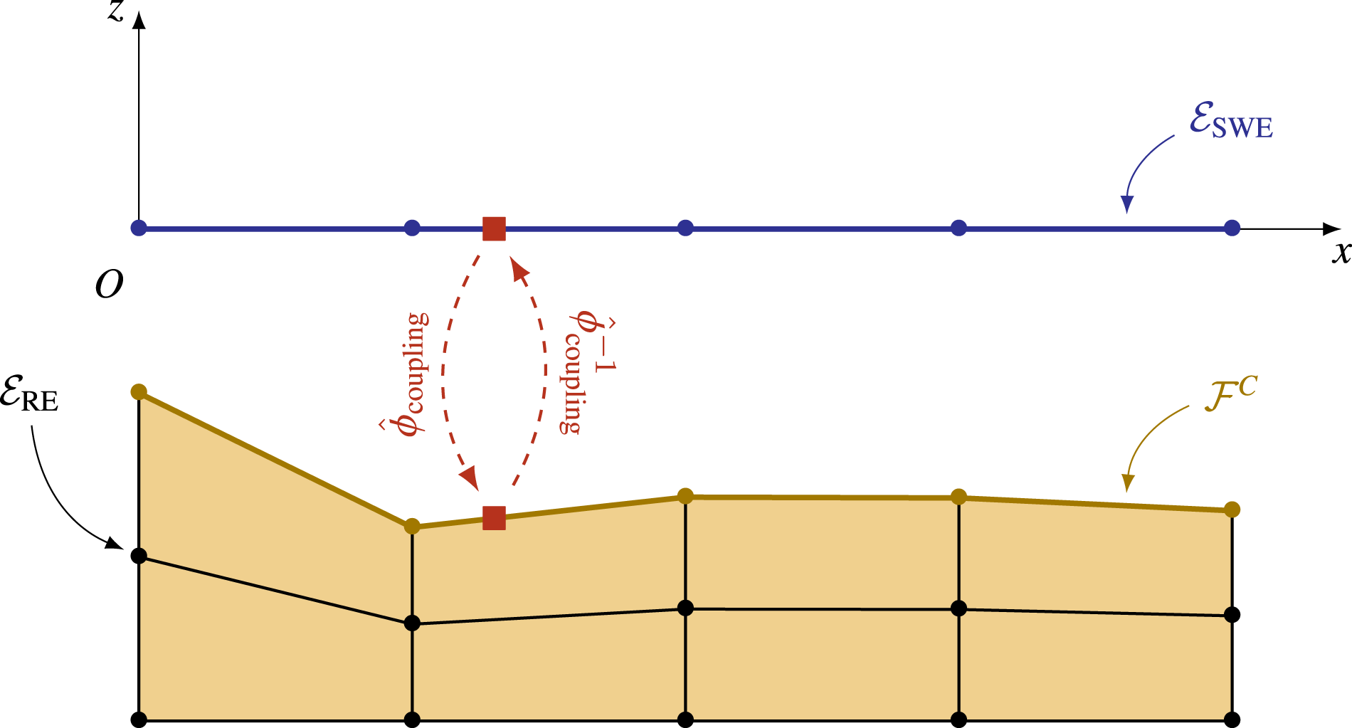
Both $Ω_{re}$ and $Ω_{swe}$ are discretized with meshes denoted as $E_{re}^{n}$ and $E_{swe}^{n}$ , where $n \in N$ indicates the time sub-interval $T^{n}$ . For $E_{re}^{n}$ , the set of boundary faces is represented as $F_{part} = F^{D} \cup F^{C} \cup F^{N}$ , where $F^{D} = F_{part} \cap Γ_{D}$ , $F^{N} = F_{part} \cap Γ_{N}$ , and $F^{C} = F_{part} \cap Γ_{C}$ . The mesh and domain representation for the coupling of SWE and RE with $d = 2$ can be seen in Figure 3. Furthermore, the two meshes are designed such that the number of blocks in $E_{swe}^{n}$ corresponds to the number of blocks composing the coupling boundary of $E_{re}^{n}$ . This design is not mandatory, but it helps the exchange of information between the two models and defines a coupling map function.

Figure 3.

Mesh and domain representation for the coupling of SWE and RE.

The resolution of SWE and RE with DG methods has been developed within the framework of adaptive mesh refinement (Poussel et al., 2024). Both models are solved on their respective meshes, which are composed of blocks that are refined at different levels. To facilitate the exchange of information, the aim is to have a conformal coupling interface. This means that each element $E$ of $E_{swe}$ should correspond to a face of $F^{C}$ . Therefore, the refinement levels of the elements of $E_{swe}$ and the elements sharing a face with $F^{C}$ need to be consistent.

Since the two meshes are distinct, to exchange information and compute the solution of RE in SWE and vice versa, a mapping function ${\hat{ϕ}}_{coupling} : Ω_{SWE} \to Γ_{C}$ is needed. This mapping function allows to evaluate the solution of RE on $Ω_{SWE}$ , and its inverse allows to evaluate the solution of SWE on $Γ_{C}$ . Recalling

V^{p} (E) := {v \in L^{2} (Ω) | v |_{E} \in P^{p} (E), \forall E \in E}

where

P^{p} (E)

stands for the set of polynomial functions of degree less than or equal to

p \in N

E

(see Pietro & Ern, 2012; Poussel et al., 2024 for further details) and using this mapping function and using DG space discretization weak formulations of System 28 is (see Poussel et al., 2024 for further details):

\begin{aligned} Find U := (h, q)^{T} \in [V^{p} (E_{SWE}^{n})]^{3} such that \forall t \in T^{n}, \forall E \in E_{SWE}^{n} and \forall φ \in [V^{p} (E_{SWE}^{n})]^{3}, \\ {\begin{aligned} \sum_{E \in E_{SWE}^{n}} \int_{E} φ (x) \partial_{t} U (x, t) d E - \sum_{E \in E_{SWE}^{n}} \int_{E} \partial_{x_{i}} φ (x) G_{i} (U (x, t)) d E \\ + \sum_{E \in E_{SWE}^{n}} \sum_{F \in F^{E}} \int_{F} φ (x) G_{F}^{*} (U (x, t)) d F = \sum_{E \in E_{SWE}^{n}} \int_{E} φ (x) S_{b} (U (x, t), {\tilde{z}}_{b} (x)) d E \\ + \sum_{E \in E_{SWE}^{n}} \int_{E} φ (x) S_{f} (U (x, t)) d E + \sum_{E \in E_{SWE}^{n}} \int_{E} φ (x) S_{RE} (U (x, t), {\tilde{z}}_{b} (x), u_{g} ({\hat{ϕ}}_{coupling} (x))) d E \end{aligned} \end{aligned}

(29)

where

{\tilde{z}}_{b}

is the projection of the bathymetry onto

V^{p}

and

G_{F}^{*}

is the numerical flux (based on the Rusanov flux) across any face

F

. In addition,

S_{b}

S_{f}

and

S_{RE}

are respectively the source terms due to bathymetry, friction and RE. The source term due to RE is computed using the map function (

{\hat{ϕ}}_{coupling}

) between

Ω_{swe}

and

Γ_{C}

. And, for RE the weak formulation is (see Poussel et al., 2024 for further details):

\begin{aligned} Find h \in V^{p} (E_{RE}^{n}) such that \forall t \in T^{n}, \forall E \in E_{RE}^{n} and \forall φ \in V^{p} (E_{RE}^{n}), \\ {\begin{aligned} \sum_{E \in E_{RE}^{n}} \int_{E} \partial_{t} θ (h - z) φ d E + \sum_{E \in E_{RE}^{n}} \int_{E} (K (h - z) \nabla h) \cdot \nabla φ d E \\ - \sum_{F \in F_{RE}^{in}} \int_{F} {[(K (h - z) \nabla h) \cdot n_{F}]} ⟦ φ ⟧ d F - \sum_{F \in F_{RE}^{D}} \int_{F} (K (h - z) \nabla h) \cdot n_{F} φ d F \\ + \sum_{F \in F_{RE}^{in}} \frac{1}{2} (\frac{σ_{E}^{i n}}{d_{E}} + \frac{σ_{E_{r}}^{i n}}{d_{E_{r}}}) \int_{F} ⟦ h ⟧ ⟦ φ ⟧ d F + \sum_{F \in F_{RE}^{C}} \frac{σ_{E}^{\partial}}{d_{E}} \int_{F} h φ d F + \sum_{F \in F_{RE}^{D}} \frac{σ_{E}^{\partial}}{d_{E}} \int_{F} h φ d F \\ = \sum_{F \in F_{RE}^{C}} \frac{σ_{E}^{\partial}}{d_{E}} \int_{F} (h + z_{b}) ({\hat{ϕ}}_{coupling}^{- 1} (x)) φ d F + \sum_{F \in F_{RE}^{D}} \frac{σ_{E}^{\partial}}{d_{E}} \int_{F} h_{D} φ d F - \sum_{F \in F_{RE}^{N}} \int_{F} q_{N} φ d F \end{aligned} \end{aligned}

(30)

where

n_{F}

E_{r}

σ_{E}^{\partial}

σ_{E}^{i n}

d_{E}

⟦ v ⟧

and

{[v]}

are respectively, a normal pointing from

E

E_{r}

, a neighboring element

E_{r}

such that

E \cap E_{r} = F

, a boundary penalty parameter, an interior penalty parameter, the diameter of an element

E

defined as the ratio between its surface and its perimeter, the jump and the average of a function

v

on a face

F \in F

\forall x \in F, ⟦ v ⟧ (x) := v_{r} (x) - v_{l} (x) and {[v]} (x) := \frac{1}{2} (v_{r} (x) + v_{l} (x))

where

v_{l} (x) := lim_{ε \to 0^{-}} v (x + ε n_{F}) and v_{r} (x) := lim_{ε \to 0^{+}} v (x + ε n_{F}), \forall x \in F .

On any boundary faces

F \in F^{\partial}

the trace of

v

is only defined on the left side of the face:

v_{l} (x) := lim_{ε \to 0^{-}} v (x + ε n_{F}), \forall x \in F

and these quantities are defined by

\forall x \in F, ⟦ v ⟧ (x) := v_{l} (x) and {[v]} (x) := v_{l} (x) .

In Problem (30),

X_{D}

and

X_{N}

stands for the Dirichlet and Neumann boundary condition on the generic variable

X

A variation exists on the boundary condition for the coupling term for RE. For now, the coupling is done using a Dirichlet boundary condition. It is well suited for problems that do not involve dry areas. In other words, problems where the porous medium is always covered by water. In the case of dry areas, a part of the porous medium is exposed to the atmosphere and imposing a Dirichlet boundary condition is not suitable. As mentioned in Clément et al. (2020) and Clément (2021), the seepage boundary condition models the interaction between the porous medium and the atmosphere. As a recall, the seepage boundary condition states that at the face exposed to the atmosphere, if an outflow occurs, then water pours out at atmospheric pressure, and otherwise, the porous medium acts as an impervious boundary; there is no flux. To implement this boundary condition, the coupling term in Problem (30) is modified as follows:

\begin{aligned} Find h \in V^{p} (E_{RE}^{n}) such that \forall t \in T^{n}, \forall E \in E_{RE}^{n} and \forall φ \in V^{p} (E_{RE}^{n}), \\ {\begin{aligned} \sum_{E \in E_{RE}^{n}} \int_{E} \partial_{t} θ (h - z) φ dE + \sum_{E \in E_{RE}^{n}} \int_{E} (K (h - z) \nabla h) \cdot \nabla φ dE \\ - \sum_{F \in F_{RE}^{in}} \int_{F} {[(K (h - z) \nabla h) \cdot n_{F}]} ⟦ φ ⟧ dF - \sum_{F \in F_{RE}^{D}} \int_{F} (K (h - z) \nabla h) \cdot n_{F} φ dF \\ + \sum_{F \in F_{RE}^{in}} \frac{1}{2} (\frac{σ_{E}^{i n}}{d_{E}} + \frac{σ_{E_{r}}^{i n}}{d_{E_{r}}}) \int_{F} ⟦ h ⟧ ⟦ φ ⟧ dF + \sum_{F \in F_{RE}^{C}} \frac{σ_{E}^{\partial}}{d_{E}} \int_{F} 1_{S C} (x) h φ dF + \sum_{F \in F_{RE}^{D}} \frac{σ_{E}^{\partial}}{d_{E}} \int_{F} h φ dF \\ = \sum_{F \in F_{RE}^{C}} \frac{σ_{E}^{\partial}}{d_{E}} \int_{F} 1_{S C} (x) (h + z_{b}) ({\hat{ϕ}}_{coupling}^{- 1} (x)) φ dF + \sum_{F \in F_{RE}^{D}} \frac{σ_{E}^{\partial}}{d_{E}} \int_{F} h_{D} φ dF - \sum_{F \in F_{RE}^{N}} \int_{F} q_{N} φ dF \end{aligned} \end{aligned}

(31)

with

1_{S C}

the indicator function of the coupling seepage boundary condition. This function is defined as follows:

1_{S C} (x) = {\begin{aligned} 1 if h ({\hat{ϕ}}_{coupling}^{- 1} (x)) > 0 or h_{g} (x) ⩾ z \\ 0 otherwise \end{aligned}

(32)

One can see that in the case of a fully wet problem Problem (31) and Problem (30) are equivalent, but in the case of dry areas the coupling seepage boundary condition becomes a classical seepage boundary condition.

Weak formulation of Problem (29) and Problem (31) are used to compute an approximated solution of the two-way coupling problem. Nevertheless, these weak formulations are still semi-discrete. Time integration needs to be performed to have fully discretized problems.

2.3. Time Synchronization

Typically, surface and groundwater flows have different time scales. In particular, for most surface water flows, the time steps needed for stability and accuracy of numerical methods are on the order of seconds to minutes. For groundwater flow, time steps are generally on the order of minutes to days. Consider that for the groundwater flow problem, its computational time is discretized with sub-intervals $T^{n} := [t^{n}, t^{n + 1}]$ with $Δ t_{RE}^{n} := t^{n + 1} - t^{n}$ . Now, each sub-interval $T^{n}$ is split into $K$ sub-intervals, with $T^{n, k} := [t^{n, k}, t^{n, k + 1}]$ for all $k = 1, \dots, K$ , where $Δ t_{SWE}^{n, k} := t^{n, k + 1} - t^{n, k}$ , and by definition $t^{n, 1} := t^{n}$ and $t^{n, K + 1} := t^{n + 1}$ . As seen in Poussel et al. (2024), the semi-discrete weak formulation of RE is time-integrated using an implicit method on $T^{n}$ , whereas the semi-discrete weak formulation of SWE is time-integrated using an explicit method on each $T^{n, k}$ . The time synchronization procedure is depicted in Figure 4, with Roman numerals enumerating the different stages. It is composed of four main steps:

Figure 4.

Scheme of time synchronization between RE and SWE for $T^{n}$ with $K = 5$ .

Figure 5.

Coupling toy problem’s configuration.

Figure 6.

Coupling toy problem’s initial mesh.

(I)

This is the first exchange of information between the two models. They exchange their respective solutions at the time $t^{n}$ . The solution is exchanged in its algebraic representation, and degrees of freedom are exchanged for memory consumption and efficiency. Since the solutions exchanged live in their respective solution spaces, the mapping function is useful for evaluating the solution of RE on $Ω_{swe}$ , and its inverse allows evaluating the solution of SWE on $Γ_{C}$ .

(II)

RE is solved on $T^{n}$ using the implicit Backward Differentiation Formula (BDF) method. The solution of SWE at $t^{n}$ is used in the boundary condition. The nonlinear iterative solver presented in Poussel et al. (2024), with adaptive time stepping, is used, and the next step of the time synchronization is performed only when the converged solution at $t^{n + 1}$ is obtained.

(III)

This is the second exchange of information between the two models. The solution of RE at $t^{n + 1}$ is exchanged to SWE following the same procedure as (I).

(IV)

SWE is solved on $T^{n, k}$ for all $k = 1, \dots, K$ using the explicit Runge–Kutta discontinuous Galerkin (RKDG) method. In the source terms of SWE, the solution of RE is linearly interpolated in time using the solution of RE at $t^{n}$ and $t^{n + 1}$ . The well-balanced property, the limiting procedure, and the flooding and drying treatment are performed as explained in Poussel et al. (2024). Time steps of SWE are computed through a Courant–Friedrichs–Lewy (CFL) condition. Thus, they are not constant and may vary from one time step to another.

One can observe that the groundwater flow is shifted backward in time since it uses the surface flow solution at $t^{n}$ to compute the solution at $t^{n + 1}$ . The benefit of this method is that the slowest problem pilots the global time stepping and consequently the amount of shift. There exists a variation in the time synchronization strategy. One can first solve SWE with the solution of RE at $t^{n}$ in source terms and then solve RE with the solution of SWE at $t^{n + 1}$ in the boundary condition. This way, the shift between the two models is displaced from RE to SWE but it is observed that the solution is not significantly impacted by this method.

Figure 7.

Coupling toy problem’s hydraulic head distribution (color grading), free surface elevation (black line), initial free surface elevation (red line) and mesh (white lines) at $t = 1 s$ .

Figure 8.

Coupling toy problem’s hydraulic head distribution (color grading), free surface elevation (black line), initial free surface elevation (red line) and mesh (white lines) at $t = 5 s$ .

Figure 9.

Coupling toy problem’s hydraulic head distribution (color grading), free surface elevation (black line), initial free surface elevation (red line) and mesh (white lines) at $t = 15 s$ .

Figure 10.

Steenhauer’s test case configuration.

3. Numerical Toy Problem End Experimental Benchmark for Validation

The coupling methodology described above and the DG methods introduced in Poussel et al. (2024) have been implemented in RIVAGE. This leads to an in-house code that solves problems involving the interactions between free-surface and groundwater flows. These newly implemented methods need to be validated. Since it is novel to couple these two models, there are few benchmarks available to validate RIVAGE. In this section, we first consider a toy problem to test whether the expected phenomena of a coupled problem are represented; this serves as a qualitative validation. Secondly, an experimental benchmark is considered to validate the code; this constitutes a quantitative validation.

Figure 11.

Steenhauer’s test case sediments (Steenhauer et al., 2011).

Table 1.

Steenhauer’s test case, physical parameters.

	$A$	$B$	$C$	$D$	$K_{s, x}$	$K_{s, z}$	$θ_{s}$	$θ_{r}$	$C_{lam}$	$C_{tur}$	$α_{BJ}$
unit	–	–	–	–	$m . s^{- 1}$	$m . s^{- 1}$	–	–	$m . s^{- 1}$	–	–
$d_{1.5}$	$5 10^{- 5}$	$2.5$	$5 10^{- 4}$	$2.5$	$1.27 10^{- 2}$	$2.54 10^{- 3}$	$0.3$	$0.0$	$0.0$	$0.01$	$0$
$d_{8.5}$	$5 10^{- 5}$	$2.0$	$5 10^{- 4}$	$2.0$	$2.45 10^{- 1}$	$4.90 10^{- 2}$	$0.3$	$0.0$	$0.0$	$0.02$	$0$

3.1. Coupled Groundwater and Free-Surface Flow: Toy Problem

The first test case is a toy problem designed to assess the coupling between groundwater and free-surface flows. The free-surface domain is one-dimensional with a flat bathymetry, while the groundwater domain is a two-dimensional rectangular domain. A traveling wave is considered over the ground domain, allowing water to flow through it. During this considered problem, several phenomena are expected to be observed:

The wave should travel freely over the ground domain;

Hydraulic head distribution should be modified by the traveling wave;

The global water level should decrease due to infiltration in the ground domain.

Figure 5 depicts the toy problem’s configuration. The ground domain (

Ω_{g}

) is a

20 \times 5 m

box with impervious sides (

q_{N} = 0 {m . s}^{- 1}

) and hydraulic head imposed on the bottom (

h_{D} = - 1 m

). The box is full of sand, saturated with water. Hydraulic properties use Vachaud’s relations in Clément (2021) with

A = 2.99 10^{6}, B = 5.0, C = 40, 000, D = 2.9, K s = 9.72 10^{- 2} {m . s}^{- 1}, θ_{s} = 0.3 and θ_{r} = 0.0

. The fluid domain (

Ω_{f}

) is a

20 m

long canal with flat bathymetry and solid walls at the ends. The two domains are linked through

Γ_{C}

. No friction is considered on the bottom of the fluid domain, hence

C_{tur} = C_{lam} = 0

and

α_{BJ} = 0

. Initial data are given by:

\forall x \in Ω_{g}, h_{g} (x, 0) = 0.4 y + 1 and \forall x \in Ω_{f}, ζ (x, 0) = 1 + 2 e^{- x^{2}} .

The problem is solved using DG methods, seeking solutions in $V^{1}$ with BDF and Runge Kutta (RK) integration methods of order 2. Block Based Adaptive Mesh Refinement (BB-AMR) techniques are applied to both SWE and RE. For the fluid domain, the adaptation criterion is based on the gradient of the water height with $β_{c} = β_{r} = 0.025$ (see Poussel et al., 2024, for instance). For the ground domain, the adaptation criterion is based on the gradient of the hydraulic head with $β_{c} = β_{r} = 0.2$ . The initial mesh is shown in Figure 6. The simulation is carried out until $T = 20 s$ . Auto-calibration of penalization parameters is employed, and moment limiters are set to the least diffusive for the SWE. The nonlinear solver’s stopping criteria are set to $ε_{1} = ε_{2} = 10^{- 6}$ .

Figures 7 to 9 display the solution of the toy problem at selected times. The hydraulic head distribution is shown in color grading, with the free surface elevation depicted in black, the initial free surface elevation in red, and the mesh in white. The figures demonstrate the expected phenomena of the toy problem: the wave travels freely over the ground domain, and its momentum is diminished due to friction from infiltration. The wave modifies the hydraulic head distribution, and the global water level decreases as a result of infiltration into the ground domain. The numerical results align with the expected phenomena. Furthermore, the Adaptive Mesh Refinement (AMR) technique tracks these phenomena effectively. The mesh is refined where the wave is located and where the hydraulic head distribution is modified, while it is coarsened where the gradient is low and where the wave has already passed.

Figure 12.

Steenhauer’s test case initial mesh.

Figure 13.

Steenhauer’s test case, hydraulic head distribution (color grading), free surface elevation (black line), water table (white line) and mesh at $t = 2.00 s$ for $d_{1.5}$ .

Figure 14.

Steenhauer’s test case, hydraulic head distribution (color grading), free surface elevation (black line), water table (white line) and mesh at $t = 3.00 s$ for $d_{1.5}$ .

Figure 15.

Steenhauer’s test case, hydraulic head distribution (color grading), free surface elevation (black line), water table (white line) and mesh at $t = 4.80 s$ for $d_{1.5}$ .

Figure 16.

Steenhauer’s test case, hydraulic head distribution (color grading), free surface elevation (black line), water table (white line) and mesh at $t = 7.00 s$ for $d_{1.5}$ .

Figure 17.

Steenhauer’s test case, comparison of numerical results $V^{1}$ (red line) with experimental results,(Steenhauer et al., 2011) (black cross) and numerical results, (Steenhauer et al., 2012) (blue triangle) for $d_{1.5}$ .

Figure 18.

Steenhauer’s test case, time series of the hydraulic head of numerical results $V^{1}$ (solid lines) and experimental results, (Steenhauer et al., 2011) (crosses) for gauges $P_{30}$ and $P_{31}$ .

Figure 19.

Steenhauer’s test case, evolution along time of time steps (left) and number of elements (right).

Figure 20.

Steenhauer’s test case, hydraulic head distribution (color grading), free surface elevation (black line), water table (white line) and mesh at $t = 2.00 s$ for $d_{8.5}$ .

Figure 21.

Steenhauer’s test case, hydraulic head distribution (color grading), free surface elevation (black line), water table (white line) and mesh at $t = 3.00 s$ for $d_{8.5}$ .

Figure 22.

Steenhauer’s test case, hydraulic head distribution (color grading), free surface elevation (black line), water table (white line) and mesh at $t = 4.20 s$ for $d_{8.5}$ .

Figure 23.

Steenhauer’s test case, hydraulic head distribution (color grading), free surface elevation (black line), water table (white line) and mesh at $t = 7.00 s$ for $d_{8.5}$ .

Figure 24.

Steenhauer’s test case, comparison of numerical results $V^{1}$ (red line) with experimental results, (Steenhauer et al., 2011) (black cross) and numerical results, (Steenhauer et al., 2012) (blue triangle) for $d_{8.5}$ .

Figure 25.

Steenhauer’s test case, time series of the hydraulic head of numerical results $V^{1}$ (solid lines) and experimental results, (Steenhauer et al., 2011) (crosses) for gauges $P_{30}$ and $P_{31}$ .

3.2. Coupled Groundwater and Free-Surface Flow: Steenhauer’s Test Case

Bore-driven swash on unsaturated coarse-grained beaches involves several interacting processes: surface flow over the beach face, infiltration into the unsaturated part of the beach, air entrapment below the wetting front, and groundwater flow. This phenomenon was observed during an experiment by Steenhauer et al. (2011). They used a $20 m$ long, $0.9 m$ high, and $0.45 m$ wide flume with a water reservoir at one end and a beach plane at the other. A bore was generated by quickly raising the gate of the reservoir. The bore propagated towards the beach, leading to a swash event typical of natural beaches. The beach had a $1 : 10$ slope and was located $4 m$ downstream of the reservoir. Figure 10 depicts a cross-section of the reservoir, illustrating the experiment’s configuration. The beach is made of sediment throughout its depth, with the top $30 mm$ bonded by a diluted water–cement–sediment mix, maintaining the permeability and roughness but preventing the sediment from moving. This experiment involves two different materials: one with a nominal diameter of $1.5 mm$ (denoted $d_{1.5}$ ) and another with $8.5 mm$ (denoted $d_{8.5}$ ). Samples of the two sediments are shown in Figure 11. The porous media is characterized by Clément (2021). Physical parameters can be found in Table 1. Shape parameters of Vachaud’s law are calibrated to have a classical shape of constitutive considering that the capillary fringe for $d_{8.5}$ is smaller than for $d_{1.5}$ . Hydraulic conductivity is extracted from the literature (Steenhauer et al., 2012) and anisotropy (with a ratio of $5$ ) is considered. Saturated and residual water content are extracted for the literature (Steenhauer et al., 2012). Friction coefficients are set empirically to match the experimental results. Lastly, $α_{BJ}$ is set to $0$ because the time scales of the problem are too different from each other.

Initial water height ( $h$ ) for the free-surface flow is given by:

\forall x \in Ω_{f}, h (x, 0) = {\begin{aligned} H_{0} m & , & if x < - 4.82 m \\ h_{0} m & , & if 4.82 m ⩽ x < - 0.62 m \\ - x / 10 m & , & if - 0.62 m ⩽ x < 0 m \\ 0.0 m & , & if x ⩾ 0 m \end{aligned}

with

H_{0} = 0.6 m

and

h_{0} = 0.062 m

. Initial hydraulic head (

h_{g}

) for the groundwater flow is given by:

\forall x \in Ω_{g}, h_{g} (x, 0) = 0.0 m .

Boundary conditions considered are for this test case are:

Solid wall at both en of $Ω_{f}$ ;

Impervious walls at left, right and bottom sides of $Ω_{g}$ ;

Coupling boundary condition on $Γ_{C}$ .

For both sediments, the problem is solved using DG methods, seeking solutions in $V^{1}$ with BDF and RK integration methods of order $2$ with $α_{CFL} = 0.9$ . The simulation is carried out until $T = 10 s$ . BB-AMR techniques are used for both SWE and RE. For the fluid domain, the adaptation criterion is based on the gradient of free surface elevation with $β_{c} = β_{r} = 0.01$ (see Poussel et al., 2024 for instance). In addition, if a block contains the shoreline, it is refined. For the ground domain, the adaptation criterion is based on the water content gradient with $β_{c} = β_{r} = 1.5$ . The initial mesh is given in Figure 12. Auto-calibration of penalization parameters and moment limiters, set to the least diffusive, are used for the SWE. For the wetting and drying treatment, slope modification is used with $h_{dry} = 10^{- 3}$ . The nonlinear solver’s stopping criteria are set to $ε_{1} = ε_{2} = 10^{- 3}$ . Time adaptation is used with $m_{i t} = 10$ , $M_{i t} = 20$ and $W_{i t} = 25$ (see Poussel et al., 2024).

Figure 26.

Steenhauer’s test case, evolution along time of time steps (left) and number of elements (right).

3.2.1. Results for

d_{1.5}

Figures 13 to 16 depicts the computed solution for $d_{1.5}$ at selected times. The water content ( $θ$ ) distribution is shown with color grading, the free surface elevation is black, the water table is white, the mesh is black and arrows shows Darcy velocity direction and magnitude. One can observe that $t = 2.00 s$ the bore reaches the beach with a height of $20 cm$ as expected and observed in the experiment (Steenhauer et al., 2011). At $t = 3.00 s$ , the bore propagates over the beach, the hydraulic head distribution is modified, and water infiltrates the porous medium. At $t = 4.80 s$ , the bore has reached its maximum covering of the beach and starts retreating, water is still infiltrating, and groundwater is moving through the sand. At $t = 7.00 s$ , the bore retreats, and the water table follows the bore. Nevertheless, water still moves vertically after the bore covers the beach. One can see that during the whole run-up of the bore, air is trapped between water infiltrating from the wave and the water table. This phenomenon is observed in the experiment.

Figure 17 compares results extracted from the work of Steenhauer et al. (2012) with numerical results computed with RIVAGE. One can observe that the free surface elevation is well recovered; however, at $t = 5.11 s$ , the maximum covering of the beach by the bore is underestimated. It may be caused by poor calibration of the friction coefficient. One can do several tests by trial and error to find the best value for the friction coefficient. One can see that the infiltration from the wave is well recovered in terms of the groundwater flow. However, in the literature, the connection between the initial water table and the infiltrating water table does not move, whereas, in our numerical results, it moves to the right.

During the experiments, gauges to record hydraulic head were placed at several locations. Figure 18 depicts time series of hydraulic head of numerical results $V^{1}$ and experimental results for gauges $P_{30}$ and $P_{31}$ placed at $x = 1180 mm$ and respectively $y = - 65.9 mm$ and $y = - 65.9 mm$ . One can see that the maximum hydraulic head value is well recovered. Nevertheless, the numerical results do not recover the overall shape of the time series. It may be due to the choice of constitutive law for the porous media and/or law parameters. There is a need to calibrate the constitutive law parameters to fit the experimental results better.

Figure 19 displays the evolution of time steps and the number of elements over time. The adaptation of time steps and the number of elements is evident. Time steps are maximum before the arrival of the bore to the beach ( $t = 2 s$ ). Then, during the whole run-up phase, time steps are reduced to catch strong non-linearities due to water infiltration from the free surface flow. Once the run-down phase begins, the time steps return to its maximum $Δ t_{amr}$ . The number of elements is evolving with time and the adaptation criteria. Evolution of the mesh can be observed in Figures 13 to 16.

3.2.2. Results for $d_{8.5}$

Figures 20 to 23 depicts the computed solution for $d_{1.5}$ at selected times. The water content ( $θ$ ) distribution is shown with color grading, the free surface elevation is black, the water table is white, the mesh is black and arrows shows Darcy velocity direction and magnitude. One can observe that $t = 2.00 s$ the bore reaches the beach with a height of $20 cm$ as expected and observed in the experiment (Steenhauer et al., 2011). At $t = 3.00 s$ , the bore propagates over the beach, the hydraulic head distribution is modified, and water infiltrates the porous medium. At $t = 4.20 s$ , the bore has reached its maximum covering of the beach and starts retreating, water is still infiltrating, and groundwater is moving through the sand. At $t = 7.00 s$ , the bore retreats, and the water table follows the bore. Nevertheless, water still moves vertically after the bore covers the beach. One can see that during the whole run-up of the bore, in this case no air is trapped between water infiltrating from the wave and the water table. This phenomenon is observed in the experiment.

Figure 24 compares results extracted from the work of Steenhauer et al. (2012) with numerical results computed with RIVAGE. One can observe that the free surface elevation is well recovered. However, the maximum covering of the beach by the bore is underestimated. It may be caused by poor calibration of the friction coefficient. One can see that the infiltration from the wave is well recovered in terms of the groundwater flow. However, in literature, the connection between the initial water table and the infiltrating water table moves slower to the right than numerical results.

During the experiments, gauges to record hydraulic head were placed at several locations. Figure 25 depicts time series of hydraulic head of numerical results $V^{1}$ and experimental results for gauges $P_{30}$ and $P_{40}$ placed respectively at $x = 1180 mm$ , $y = - 67.8 mm$ and $x = 1980 mm$ , $y = - 65.1 mm$ . One can see that the maximum hydraulic head value is well recovered. Nevertheless, the numerical results do not recover the overall shape of the time series. It may be due to the choice of constitutive law for the porous media and/or law parameters.

Figure 26 displays the evolution of time steps and the number of elements over time. The adaptation of time steps and the number of elements is evident. Time steps are maximum before the arrival of the bore to the beach ( $t = 2 s$ ). Then, during the whole run-up phase, time steps are reduced to catch strong non-linearities due to water infiltration from the free surface flow. Once the run-down phase begins, the time steps return to its maximum $Δ t_{amr}$ . The number of elements is evolving with time and the adaptation criteria. Evolution of the mesh can be observed in Figures 20 to 23.

Footnotes

ORCID iD

Camille Poussel

Funding

The authors disclosed receipt of the following financial support for the research, authorship, and/or publication of this article: The work received France 2030 funding under the reference “ANR-23-EXMA-0007.”

Declaration of Conflicting Interests

The authors declared no potential conflicts of interest with respect to the research, authorship, and/or publication of this article.

Appendix

References

Anderson

Woessner

Hunt

(2015). Applied ground water modeling: Simulation of flow and advective transport .

Beavers

G. S.

Joseph

D. D.

(1967). Boundary conditions at a naturally permeable wall. Journal of Fluid Mechanics, 30(1), 197–207. https://doi.org/10.1017/S0022112067001375

Cardenas

M. B.

Zlotnik

V. A.

(2003). Three-dimensional model of modern channel bend deposits. Water Resources Research, 39(6). https://doi.org/10.1029/2002WR001383

Caviedes-Voullième

Murillo

Garcia-Navarro

(2012). Numerical simulation of groundwater- surface interactions by external coupling of the 3D Richards equation and the full 2D shallow-water equations.

Clément

J.-B.

(2021). Numerical simulation of flows in unsaturated porous media by an adaptive discontinuous Galerkin method: Application to sandy beaches. PhD thesis, Université de Toulon.

Clément

J.-B.

Golay

Ersoy

Sous

(2020). Adaptive discontinuous Galerkin method for Richards equation. In Topical problems of fluid mechanics 2020, (pp. 27–34), Prague, Czech Republic. Institute of Thermomechanics, AS CR, v.v.i. https://hal.science/hal-02507326, DOI: https://doi.org/10.14311/TPFM.2020.004.

Clément

J.-B.

Golay

Ersoy

Sous

(2021). An adaptive strategy for discontinuous Galerkin simulations of Richards’ equation: Application to multi-materials dam wetting. Advances in Water Resources, 151, 103897. https://doi.org/10.1016/j.advwatres.2021.103897

Dawson

(2008). A continuous/discontinuous Galerkin framework for modeling coupled subsurface and surface water flow. Computational Geosciences, 12(4), 451–472. https://doi.org/10.1007/s10596-008-9085-y

Delestre

(2010). Simulation du ruissellement D’eau De pluie sur des surfaces agricoles. PhD thesis, Université d’Orléans.

10.

Delpierre

Rattez

Soares-Frazao

(2023). Finite-volume coupled surface-subsurface flow modelling in earth dikes. Journal of Hydraulic Research, 61(5), 754–763. https://doi.org/10.1080/00221686.2023.2246936

11.

Discacciati

Miglio

Quarteroni

(2002). Mathematical and numerical models for coupling surface and groundwater flows. Applied Numerical Mathematics, 43(1), 57–74. https://doi.org/10.1016/S0168-9274(02)00125-3

12.

Discacciati

Quarteroni

(2009). Navier–Stokes/Darcy coupling: Modeling, analysis, and numerical approximation. Revista Matemática Complutense, 22, 315–426. https://doi.org/10.5209/rev_REMA.2009.v22.n2.16263

13.

Dong

Zhang

Bai

(2013). A hybrid coupled model of surface and subsurface flow for surface irrigation. Journal of Hydrology, 500, 62–74. https://doi.org/10.1016/j.jhydrol.2013.07.018

14.

Ersoy

Lakkis

Townsend

(2021). A Saint–Venant model for overland flows with precipitation and recharge. Mathematical and Computational Applications, 26(1), 1. https://doi.org/10.3390/mca26010001

15.

Freeze

R. A.

Harlan

R. L.

(1969). Blueprint for a physically-based, digitally-simulated hydrologic response model. Journal of Hydrology, 9(3), 237–258. https://doi.org/10.1016/0022-1694(69)90020-1

16.

Furman

(2008). Modeling coupled surface–subsurface flow processes: A review. Vadose Zone Journal, 7(2), 741–756. https://doi.org/10.2136/vzj2007.0065

17.

Girault

Rivière

(2009). DG approximation of coupled Navier–Stokes and Darcy equations by Beaver–Joseph–Saffman interface condition. SIAM Journal on Numerical Analysis, 47(3), 2052–2089. https://doi.org/10.1137/070686081

18.

Layton

W. J.

Schieweck

Yotov

(2002). Coupling fluid flow with porous media flow. SIAM Journal on Numerical Analysis, 40(6), 2195–2218. https://doi.org/10.1137/S0036142901392766

19.

Marche

(2007). Derivation of a new two-dimensional viscous shallow water model with varying topography, bottom friction and capillary effects. European Journal of Mechanics - B. Fluids, 26(1), 49–63. https://doi.org/10.1016/j.euromechflu.2006.04.007

20.

Mikelic

Jäger

(2000). On the interface boundary condition of Beavers, Joseph, and Saffman. SIAM Journal on Applied Mathematics, 60(4), 1111–1127. https://doi.org/10.1137/S003613999833678X

21.

Morita

Yen

B. C.

(2000). Numerical methods for conjunctive two-dimensional surface and three-dimensional sub-surface flows. International Journal for Numerical Methods in Fluids, 32(8), 921–957. https://doi.org/10.1002/(SICI)1097-0363(20000430)32:8<921::AID-FLD993=3.0.CO;2-3

22.

Pietro

D. A. D.

Ern

(2012). Mathematical aspects of discontinuous galerkin methods.

23.

Pons

(2018). Modélisation des tsunamis: Propagation et impact PhD thesis, Université de Toulon. Springer.

24.

Poussel

Ersoy

Golay

(2024). Wetting and drying treatments with mesh adaptation for shallow water equations using a Runge–Kutta discontinuous Galerkin method. Working paper or preprint. https://hal.science/hal-04676186.

25.

Pringle

W. J.

Yoneyama

Mori

(2016). Two-way coupled long wave—RANS model: Solitary wave transformation and breaking on a plane beach. Coastal Engineering, 114, 99–118. https://doi.org/10.1016/j.coastaleng.2016.04.011

26.

Richards

L. A.

(1931). Capillary conduction of liquids through porous mediums. Physics, 1(5), 318–333. https://doi.org/10.1063/1.1745010

27.

Richardson

L. F.

(1922). Weather prediction by numerical process. Cambridge University Press.

28.

Rivière

Yotov

(2005). Locally conservative coupling of Stokes and Darcy flows. SIAM Journal on Numerical Analysis, 42(5), 1959–1977. https://doi.org/10.1137/S0036142903427640

29.

Saffman

P. G.

(1971). On the boundary condition at the surface of a porous medium. Studies in Applied Mathematics, 50(2), 93–101. https://doi.org/10.1002/sapm197150293

30.

Steenhauer

Pokrajac

O’Donoghue

(2012). Numerical model of swash motion and air entrapment within coarse-grained beaches. Coastal Engineering, 64, 113–126. https://doi.org/10.1016/j.coastaleng.2012.01.004

31.

Steenhauer

Pokrajac

O’Donoghue

Kikkert

G. A.

(2011). Subsurface processes generated by bore-driven swash on coarse-grained beaches. Journal of Geophysical Research: Oceans, 116(C4). https://doi.org/10.1029/2010JC006789

32.

Todd

D. K.

(1980). Groundwater hydrology. Geological Magazine, 118(4), 442. https://doi.org/10.1017/S0016756800032477

33.

VanderKwaak

J. E.

Loague

(2001). Hydrologic-response simulations for the R-5 catchment with a comprehensive physics-based model. Water Resources Research, 37(4), 999–1013. https://doi.org/10.1029/2000WR900272

34.

Yeh

G.-T.

Cheng

H.-P.

Cheng

Lin

Martin

(1998). A numerical model simulating water flow and contaminant and sediment transport in WAterSHed systems of 1-D stream-river network, 2-D overland regime, and 3-D Subsurface Media (WASH123D: Version 1.0).

Derivation of the Nonlinear Shallow Water Equations Over Unsaturated Porous Media: A Discontinuous Galerkin Method for Coarse-Grained Beaches

Abstract

Keywords

1. Derivation of the Coupled Model

2.1. Coupling Methods

3.2.2. Results for d 8.5

Footnotes

ORCID iD

Funding

Declaration of Conflicting Interests

Appendix

References

3.2.2. Results for $d_{8.5}$