Stability of Thermoelastic Plates With Voids and Micro-Temperatures

Abstract

We study the asymptotic behaviour of thermoelastic plates with voids where the thermal effects include micro-temperatures. Under suitable conditions on the constitutive constants, we prove well-posedness of the problem by means of semigroup theory. Also we prove that the solutions decay in an exponential way by means of Prüss characterisations of exponential stable semigroups. Later the regularity of the solutions is studied and we see that the semigroup is not differentiable. The case when certain coupling terms vanish is also considered and polynomial decay estimates are obtained.

Keywords

thermoelasticity asymptotic analysis stability micro-temperatures materials with voids

1. Introduction

It has been more than 50 years since the asymptotic behaviour of thermoelasticity problems began to be investigated (Dafermos, 1976). Usually a system of equations is considered in which conservative structures and dissipative structures are combined and the objective is to see how the latter drag the entire system to a situation of equilibrium. At the same time, knowledge of the regularity of the solutions is usually an objective associated with this type of studies.

A sub-class of these problems is determined by the study of plates. This goal has seen many contributions recently. We can assure that if the equation that determines the heat equation is parabolic, the solutions of the system decay exponentially and are analytical (Liu & Quintanilla, 2010; Liu & Renardy, 1995; Liu et al., 2022). However, if the heat equation is hyperbolic, the decay is slower (Quintanilla & Racke, 2011). We know an exception to this last statement that corresponds to the case that the heat equation is determined by the Green–Lindsay theory (Green & Lindsay, 1972), in which case we also have exponential decay since in that case the coupling is stronger (Quintanilla et al., 2023).

In recent years we have seen how the decay of solutions, in the case of plates, other mechanisms were incorporated such as porosity (Fernández Sare & Quintanilla, 2021). Our article aims to continue along this line. We know that even in the case that heat conduction is determined by Fourier’s law, if we include porosity, the decay of the solutions is not exponential. Therefore, it is natural to introduce another type of mechanism that allows for the conclusion of an exponential decay. This problem was considered for the usual thermoelasticity in the one-dimensional case and it was demonstrated (Casas & Quintanilla, 2005) that microtemperatures (Ieşan & Quintanilla, 2000) are a mechanism that allows this type of decay to be concluded. We can ask ourselves if a similar phenomenon occurs in the case of plates as well as have knowledge of the regularity of the solutions.

In this work we will demonstrate that (generally) the decay of thermoelastic plates with porosity and microtemperatures is exponential. However, the semigroup that generates the solutions to the problem is not differentiable. Finally, we will also obtain decay estimators (of polynomial type) in the case that some of the coupling mechanisms are not present.

The article is organised as follows. In Section 2 we propose the mathematical model that we study in this article, also we do some remarks about the constitutive energy of the system. In Section 3 we establish the well-posedness of the system introducing it in a semigroup context. In Section 4, assuming the presence of the high order coupling term $μ_{2} \neq 0$ , we prove exponential stability of solutions. Finally, in Section 5.2 we consider the cases of weak coupling terms, proving not exponential stability for the case $β = 0$ or $μ_{2} = 0$ . Also, in the presence of the high order coupling term $μ_{2}$ , we prove that the corresponding semigroup is not differentiable. The article ends by giving several polynomial estimates in the cases where $β = 0$ or $μ_{2} = 0$ .

2. Model

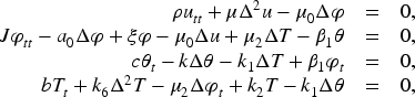
In this section we propose the initial boundary value problem which will be the target of study of our article. We consider a thermoelastic plate which also includes porosity effects (see Cowin, 1985; Cowin & Nunziato, 1983), and micro-temperatures (see Ieşan, 2007; Ieşan & Quintanilla, 2000). This is, the system of equations can be written as

\begin{array}{rcl} ρ u_{t t} + μ Δ^{2} u - μ_{0} Δ φ + β Δ θ & = & 0, \\ J φ_{t t} - a_{0} Δ φ + ξ φ - μ_{0} Δ u + μ_{2} Δ T - β_{1} θ & = & 0, \\ c θ_{t} - k Δ θ - k_{1} Δ T - β Δ u_{t} + β_{1} φ_{t} & = & 0, \\ b T_{t} + k_{6} Δ^{2} T - μ_{2} Δ φ_{t} + k_{2} T - k_{1} Δ θ & = & 0, \end{array}

(1)

with associated boundary conditions

\begin{array}{rcl} u (x, t) = Δ u (x, t) = φ (x, t) & = & 0 in \partial Ω \times R^{+} \\ θ (x, t) = T (x, t) = Δ T (x, t) & = & 0 in \partial Ω \times R^{+}, \end{array}

(2)

and initial conditions

\begin{array}{cl} u (\cdot, 0) = u_{0} (\cdot), u_{t} (\cdot, 0) = u_{1} (\cdot) & in Ω, \\ φ (\cdot, 0) = φ_{0} (\cdot), φ_{t} (\cdot, 0) = φ_{1} (\cdot) & in Ω, \\ θ (\cdot, 0) = θ_{0} (\cdot), T (\cdot, 0) = T_{0} (\cdot) & in Ω . \end{array}

(3)

In this system

u

models the displacement,

φ

the volume fraction,

θ

and

T

are the temperature and the micro-temperature, respectively. For the coefficients,

ρ

represents the mass density,

J

the product of the mass density by the equilibrated inertia,

c

is the heat capacity and

b

is a similar parameter corresponding to the micro-temperature;

μ

is the elasticity coefficient with

a_{0}

playing a similar role for the porosity;

k

is the thermal conductivity and

k_{6}

is the similar parameter for the micro-temperature;

ξ

is a parameter related to the porosity and

k_{2}

to the micro-temperature. The rest of the parameters represent different couplings between the variables.

Here, the hypotheses on the constitutive constants are given by

\begin{matrix} ρ, μ, J, a_{0}, ξ, c, b, k, k_{6} > 0, k_{1}, k_{2} \geq 0, μ_{0}, μ_{2}, β, β_{1} \in R, μ ξ > μ_{0}^{2}, \\ k > | k_{1} | and min {k_{2}, k_{6}} > \frac{| k_{1} |}{2} . \end{matrix}

(4)

The last two conditions in (4) are formulated to show that the dissipation of the system is positive. In fact, note that the energy of the system, using appropriate boundary conditions, is given by

E (t) = \frac{1}{2} \int_{Ω} [ρ | u_{t} |^{2} + μ | Δ u |^{2} + J | φ_{t} |^{2} + a_{0} | \nabla φ |^{2} + ξ | φ |^{2} - 2 μ_{0} (Δ u) φ + c | θ |^{2} + b | T |^{2}] d x,

(5)

which satisfies

\frac{d}{d t} E (t) = - k \int_{Ω} | \nabla θ |^{2} d x + 2 k_{1} \int_{Ω} \nabla T . \nabla θ d x - k_{6} \int_{Ω} | Δ T |^{2} d x - k_{2} \int_{Ω} | T |^{2} d x .

So, noting that

| 2 k_{1} \int_{Ω} \nabla T . \nabla θ d x | \leq | k_{1} | \int_{Ω} | \nabla θ |^{2} d x + | k_{1} | \int_{Ω} | \nabla T |^{2} d x,

with

| k_{1} | \int_{Ω} | \nabla T |^{2} d x = | - | k_{1} | \int_{Ω} Δ T T d x | \leq \frac{| k_{1} |}{2} \int_{Ω} | Δ T |^{2} d x + \frac{| k_{1} |}{2} \int_{Ω} | T |^{2} d x .

So, substituting into (5) we obtain

\frac{d}{d t} E (t) \leq - (k - | k_{1} |) \int_{Ω} | \nabla θ |^{2} d x - (k_{6} - \frac{| k_{1} |}{2}) \int_{Ω} | Δ T |^{2} d x - (k_{2} - \frac{| k_{1} |}{2}) \int_{Ω} | T |^{2} d x,

(6)

which defines the dissipative characteristic of the energy of the system.

Remark 2.1

In general, conditions on $k_{1}$ , $k_{2}$ and $k_{6}$ given into (4) can be generalised to other infinite situations. That is, we can consider for any fixed but arbitrary $ε_{1}, ε_{2} > 0$ , the conditions

k > | k_{1} | ε_{1}, k_{2} > \frac{| k_{1} |}{2 ε_{1} ε_{2}} and k_{6} > \frac{| k_{1} | ε_{2}}{2 ε_{1}} .

(7)

In this case, (6) is rewritten as

\frac{d}{d t} E (t) \leq - (k - | k_{1} | ε_{1}) \int_{Ω} | \nabla θ |^{2} d x - (k_{6} - \frac{| k_{1} | ε_{2}}{2 ε_{1}}) \int_{Ω} | Δ T |^{2} d x - (k_{2} - \frac{| k_{1} |}{2 ε_{1} ε_{2}}) \int_{Ω} | T |^{2} d x,

which keeps the dissipative characteristic of the energy. In this article, without loss of generality, we use condition (4) just to simplify the notation. Nevertheless, our results can be generalised to all situation given by (7).

3. Semigroup Context

Let use denote by $Ω$ a two-dimensional domain with boundary smooth enough to apply the divergence theorem and compactness embeddings. Now, let us embed the system in a semigroup context, necessary to use well-know characterisations of exponentially stable semigroups (see Prüss, 1984 for example). In fact, we formulate the system as an abstract Cauchy problem by using the notation $U := (u, v, φ, ψ, θ, T)^{'}$ , with $v = u_{t}$ and $ψ = φ_{t}$ . So, systems (1)–(3) is equivalent to

U_{t} = A U, U (0) = U_{0},

(8)

where

U_{0} = (u_{0}, u_{1}, φ_{0}, φ_{1}, θ_{0}, T_{0})^{'}

and

A

is the corresponding matrix operator

\begin{aligned} A (\begin{matrix} u \\ v \\ φ \\ ψ \\ θ \\ T \end{matrix}) = (\begin{matrix} v \\ - \frac{1}{ρ} [μ Δ^{2} u - μ_{0} Δ φ + m Δ θ] \\ ψ \\ - \frac{1}{J} [- a_{0} Δ φ + ξ φ - μ_{0} Δ u + μ_{2} Δ T - β_{1} θ] \\ - \frac{1}{c} [- k Δ θ - k_{1} Δ T - β Δ v + β_{1} ψ] \\ - \frac{1}{b} [k_{6} Δ^{2} T - μ_{2} Δ ψ + k_{2} T - k_{1} Δ θ] \end{matrix}) . \end{aligned}

We define the Hilbert space

H := [H^{2} (Ω) \cap H_{0}^{1} (Ω)] \times L^{2} (Ω) \times H_{0}^{1} (Ω) \times L^{2} (Ω) \times L^{2} (Ω) \times L^{2} (Ω),

with inner product, for

U_{i} = (u_{i}, v_{i}, φ_{i}, ψ_{i}, θ_{i}, T_{i})^{T}

i = 1, 2

, given by

\begin{aligned} (U_{1}, U_{2})_{H} = & ρ (v_{1}, v_{2})_{L^{2}} + μ (Δ u_{1}, Δ u_{2})_{L^{2}} + J (ψ_{1}, ψ_{2})_{L^{2}} + a_{0} (\nabla φ_{1}, \nabla φ_{2})_{L^{2}} + ξ (φ_{1}, φ_{2})_{L^{2}} \\ - μ_{0} (φ_{1}, Δ u_{1})_{L^{2}} - μ_{0} (Δ u_{2}, φ_{2})_{L^{2}} + c (θ_{1}, θ_{2})_{L^{2}} + b (T_{1}, T_{2})_{L^{2}} . \end{aligned}

Then, using condition (4),

H

is a Hilbert space with the norm, for

U = (u, v, φ, ψ, θ, T)^{T}

, given by

\begin{aligned} | | U | |_{H}^{2} = & ρ | | v | |_{L^{2}}^{2} + μ | | Δ u | |_{L^{2}}^{2} + J | | ψ | |_{L^{2}}^{2} + a_{0} | | \nabla φ | |_{L^{2}}^{2} + ξ | | φ | |_{L^{2}}^{2} \\ - 2 μ_{0} Re (Δ u, φ)_{L^{2}} + c | | θ | |_{L^{2}}^{2} + b | | T | |_{L^{2}}^{2} . \end{aligned}

Here, the domain of operator

A

is given by

\begin{aligned} D (A) = & {(u, v, φ, ψ, θ, T)^{T} \in [H^{4} (Ω) \cap H_{0}^{1} (Ω)] \times [H^{2} (Ω) \cap H_{0}^{1} (Ω)]^{4} \times [H^{4} (Ω) \cap H_{0}^{1} (Ω)] \\ such that Δ u = Δ T = 0 on \partial Ω} . \end{aligned}

First of all, using similar arguments used to obtain (6), that

\begin{aligned} Re (A U, U)_{H} = & - k | | \nabla θ | |_{L^{2}}^{2} - k_{6} | | Δ T | |_{L^{2}}^{2} - k_{2} | | T | |_{L^{2}}^{2} + 2 k_{1} Re (Δ T, θ)_{L^{2}} \\ \leq & - (k - | k_{1} |) | | \nabla θ | |_{L^{2}}^{2} - (k_{6} - \frac{| k_{1} |}{2}) | | Δ T | |_{L^{2}}^{2} - (k_{2} - \frac{| k_{1} |}{2}) | | T | |_{L^{2}}^{2}, \end{aligned}

for all

U \in D (A)

, which implies that

A

is a dissipative operator. Also, using Lax Milgram’s Theorem we conclude that

0 \in ϱ (A)

In this context, a direct consequence of Lumer–Phillips theorem (see Pazy, 1983), implies the following well-posedness result.

Theorem 3.1

The operator $A$ is the infinitesimal generator of a $C_{0}$ -semigroup of contractions. As consequence, the evolution problem (8) is well-posed, this is, for all initial data $U_{0} \in D (A)$ , there exists an unique strong solution $U$ of (8) satisfying the regularity

U \in C (R^{+}; D (A)) \cap C^{1} (R^{+}; H) .

4. Exponential Stability

In this section, assuming that $β \neq 0$ and $μ_{2} \neq 0$ , we will prove that systems (1)–(3) is exponentially stable. For this purpose, we use the following characterisation of exponentially stable semigroups:

Theorem 4.1
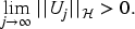
Let $T (t) = e^{A t}$ $(t \geq 0)$ , a semigroup of contractions on the Hilbert space $H$ with generator $A$ and associated norm $| | \cdot | |_{H}$ . Then ${T (t)}_{t \geq 0}$ is exponentially stable if and only if
$i R \subset ϱ (A)$
(9)
and
$\underset{| λ | \to \infty}{lim sup} | | (i λ I - A)^{- 1} | |_{L (H, H)} < \infty .$
(10)
Proof.
See Huang (1985), Liu and Zheng (1999) and Prüss (1984).

In fact, first we show (9) using contradiction arguments, this is, supposing that (9) is not true. Then (cp. Liu & Zheng, 1999, pg. 25) there exists $ω \in R$ , a sequence $(ω_{n})_{n} \subset R$ with $ω_{n} \to ω$ , $| ω_{n} | < ω$ and a sequence of functions
$U_{n} = {(u_{n}, v_{n}, φ_{n}, ψ_{n}, θ_{n}, T_{n})}^{'} \in D (A) with | | U_{n} | |_{H} = 1$
(11)
such that
$i ω_{n} U_{n} - A U_{n} ⟶ 0 in H, (n \to \infty)$
(12)
that is,
$\begin{aligned} i ω_{n} u_{n} - v_{n} \to & 0 in H^{2} (Ω) \cap H_{0}^{1} (Ω) \end{aligned}$
(13)

$\begin{aligned} i ω_{n} ρ v_{n} + μ Δ^{2} u_{n} - μ_{0} Δ φ_{n} + β Δ θ_{n} \to & 0 in L^{2} (Ω) \end{aligned}$
(14)

$\begin{aligned} i ω_{n} φ_{n} - ψ_{n} \to & 0 in H_{0}^{1} (Ω) \end{aligned}$
(15)

$\begin{aligned} i ω_{n} J ψ_{n} - a_{0} Δ φ_{n} + ξ φ_{n} - μ_{0} Δ u_{n} + μ_{2} Δ T_{n} - β_{1} θ_{n} \to & 0 in L^{2} (Ω) \end{aligned}$
(16)

$\begin{aligned} i ω_{n} c θ_{n} - k Δ θ_{n} - k_{1} Δ T_{n} - β Δ v_{n} + β_{1} ψ_{n} \to & 0 in L^{2} (Ω) \end{aligned}$
(17)

$\begin{aligned} i ω_{n} b T_{n} + k_{6} Δ^{2} T_{n} - μ_{2} Δ ψ_{n} + k_{2} T_{n} - k_{1} Δ θ_{n} \to & 0 in L^{2} (Ω) . \end{aligned}$
(18)
Taking the inner product of (12) with $U_{n}$ in $A$ and then taking its real part yields
$Re (A U_{n}, U_{n})_{H} = k | | \nabla θ_{n} | |_{L^{2}}^{2} + k_{6} | | Δ T_{n} | |_{L^{2}}^{2} + k_{2} | | T_{n} | |_{L^{2}}^{2} - 2 k_{1} Re (Δ T_{n}, θ_{n})_{L^{2}} ⟶ 0.$
(19)
Similar to the previous sections, note that
$| - 2 k_{1} Re (Δ T_{n}, θ_{n})_{L^{2}} | \leq | k_{1} | | | \nabla θ_{n} | |_{L^{2}}^{2} + \frac{| k_{1} |}{2} | | Δ T_{n} | |_{L^{2}}^{2} + \frac{| k_{1} |}{2} | | T_{n} | |_{L^{2}}^{2},$
which implies
$- | k_{1} | | | \nabla θ_{n} | |_{L^{2}}^{2} - \frac{| k_{1} |}{2} | | Δ T_{n} | |_{L^{2}}^{2} - \frac{| k_{1} |}{2} | | T_{n} | |_{L^{2}}^{2} \leq - 2 k_{1} Re (Δ T_{n}, θ_{n})_{L^{2}} ⟶ 0.$
(20)
So, combining (19) and (20), we obtain
$(k - | k_{1} |) | | \nabla θ_{n} | |_{L^{2}}^{2} + (k_{6} - \frac{| k_{1} |}{2}) | | Δ T_{n} | |_{L^{2}}^{2} + (k_{2} - \frac{| k_{1} |}{2}) | | T_{n} | |_{L^{2}}^{2} \leq Re (A U_{n}, U_{n})_{H} ⟶ 0.$
Consequently,
$θ_{n} ⟶ 0 in H_{0}^{1} (Ω) and T_{n} ⟶ 0 in H^{2} (Ω) \cap H_{0}^{1} (Ω) .$
(21)

On the other hand, let us define a sequence $(z_{n})_{n \in N}$ as the family of solutions of the elliptic problems
$- Δ z_{n} = ψ_{n}, z_{n} = 0 on \partial Ω .$
Note that $(z_{n})_{n \in N}$ is bounded in $H_{0}^{1} (Ω)$ because $(ψ_{n})_{n \in N}$ is bounded in $L^{2} (Ω)$ . So, multiplying (18) by $z_{n}$ in $L^{2} (Ω)$ we obtain
$i ω_{n} b (T_{n}, z_{n})_{L^{2}} - k_{6} (Δ T_{n}, ψ_{n})_{L^{2}} + μ_{2} | | ψ_{n} | |_{L^{2}}^{2} + k_{2} (T_{n}, z_{n})_{L^{2}} + k_{1} (\nabla θ_{n}, \nabla z_{n})_{L^{2}} ⟶ 0,$
which implies, using (21), that
$ψ_{n} ⟶ 0 in L^{2} (Ω) .$
(22)
Also, combining (15) and (22) we obtain
$φ_{n} ⟶ 0 in L^{2} (Ω) .$
(23)
Now, let us define an additional sequence $(z_{n})_{n \in N}$ , bounded in $H_{0}^{1} (Ω)$ , given by the solutions of the elliptic problems
$- Δ z_{n} = v_{n}, z_{n} = 0 on \partial Ω .$
(24)
So, multiplying (17) by $z_{n}$ in $L^{2} (Ω)$ and using (21) and (22), we obtain
$v_{n} ⟶ 0 in L^{2} (Ω) .$
(25)
Also, multiplying (14) by $u_{n}$ in $L^{2} (Ω)$ we obtain
$i ω_{n} ρ (v_{n}, u_{n})_{L^{2}} + μ | | Δ u_{n} | |_{L^{2}}^{2} - μ_{0} (φ_{n}, Δ u_{n})_{L^{2}} + β (θ_{n}, Δ u_{n})_{L^{2}} \to 0,$
which implies, using (21), (23) and (25), that
$u_{n} ⟶ 0 in H^{2} (Ω) \cap H_{0}^{1} (Ω) .$
(26)
Moreover, multiplying (16) by $φ$ in $L^{2} (Ω)$ and using (21), (22) and (26) we deduce
$φ_{n} ⟶ 0 in H_{0}^{1} (Ω) .$
(27)
So, combining (21), (22), (25), (26) and (27) we obtain
$U_{n} ⟶ 0 in H,$
which is a contradiction with $| | U_{n} | |_{H} = 1$ given by (11). Consequently, condition (9) holds.

Now, in order to complete the result about exponential stability, we now prove (10). Note that the resolvent equation
$(i λ I - A) U = F \in H$
(28)
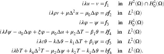
is given by
$\begin{aligned} i λ u - v = & f_{1} in H^{2} (Ω) \cap H_{0}^{1} (Ω) \end{aligned}$
(29)

$\begin{aligned} i λ ρ v + μ Δ^{2} u - μ_{0} Δ φ + β Δ θ = & ρ f_{2} in L^{2} (Ω) \end{aligned}$
(30)

$\begin{aligned} i λ φ - ψ = & f_{3} in H_{0}^{1} (Ω) \end{aligned}$
(31)

$\begin{aligned} i λ J ψ - a_{0} Δ φ + ξ φ - μ_{0} Δ u + μ_{2} Δ T - β_{1} θ = & J f_{4} in L^{2} (Ω) \end{aligned}$
(32)

$\begin{aligned} i λ c θ - k Δ θ - k_{1} Δ T - β Δ v + β_{1} ψ = & c f_{5} in L^{2} (Ω) \end{aligned}$
(33)

$\begin{aligned} i λ b T + k_{6} Δ^{2} T - μ_{2} Δ ψ + k_{2} T - k_{1} Δ θ = & b f_{6} in L^{2} (Ω) . \end{aligned}$
(34)

In order to simplify our analysis, let us introduce the multipliers $z$ , $y$ , $η$ and $w$ defined as solutions of the following elliptic equations
${\begin{array}{lcr} - Δ z = v in Ω, & z = 0 in \partial Ω, \\ - Δ y = ψ in Ω, & y = 0 in \partial Ω, \\ - Δ η = θ in Ω, & η = 0 in \partial Ω, \\ - Δ w = T in Ω, & w = 0 in \partial Ω . \end{array}$
(35)
Then, there exists $C > 0$ such that
$\begin{aligned} {\begin{array}{rcl} | | z | |_{H_{0}^{1}} & \leq & C | | v | |_{L^{2}}, \\ | | y | |_{H_{0}^{1}} & \leq & C | | ψ | |_{L^{2}}, \\ | | η | |_{H_{0}^{1}} & \leq & C | | θ | |_{L^{2}}, \\ | | w | |_{H_{0}^{1}} & \leq & C | | T | |_{L^{2}} . \end{array} \end{aligned}$
(36)
In what follows we will use the notation $C > 0$ to represent a constant always independent of $λ$ , $U$ and $F$ . To prove (10) we divide our analysis in some lemmas.
Lemma 4.2
For all $U = (u, v, φ, ψ, θ, T)^{'} \in D (A)$ , there exists a positive constant $C$ , being independent of $F$ such that
$| | \nabla θ | |_{L^{2}}^{2} + | | Δ T | |_{L^{2}}^{2} + | | T | |_{L^{2}}^{2} \leq C | | U | |_{H} | | F | |_{H} .$
(37)
Proof.
This inequality is a direct consequence of the dissipative condition of operator $A$ and it is obtained multiplying the resolvent equation (28) by $U$ in space $H$ , taking the real part and using similar arguments used to obtain (6).
Lemma 4.3
Assuming $μ_{2} \neq 0$ , for all $U = (u, v, φ, ψ, θ, T)^{'} \in D (A)$ , there exists a positive constant $C$ , being independent of $F$ such that
$| | ψ | |_{L^{2}}^{2} \leq C | | U | |_{H} | | F | |_{H} + C | | U | |_{H}^{1 / 2} | | F | |_{H}^{1 / 2} (| | φ | |_{L^{2}} + | | Δ u | |_{L^{2}}) .$

Proof.
Multiplying (34) by $y$ and using (35) we obtain
$\underset{I_{1}}{\underset{⏟}{i λ b (T, y)_{L^{2}}}} - k_{6} (Δ T, ψ)_{L^{2}} + μ_{2} | | ψ | |_{L^{2}}^{2} + k_{2} (T, y) + k_{1} (\nabla θ, \nabla y)_{L^{2}} = b (f_{6}, y)_{L^{2}}$
(38)
Then, from (32) and taking into account $y$ and $w$ given in (35), we obtain
$\begin{aligned} I_{1} = & i λ b (Δ w, y)_{L^{2}} = b (w, - i λ ψ)_{L^{2}} \\ = & \frac{b}{J} (w, - a_{0} Δ φ + ξ φ - μ_{0} Δ u + μ_{2} Δ T - β_{1} θ - J f_{4})_{L^{2}} \\ = & \frac{a_{0} b}{J} (T, φ)_{L^{2}} + \frac{b ξ}{J} (w, φ)_{L^{2}} - \frac{b μ_{0}}{J} (w, Δ u)_{L^{2}} + \frac{b μ_{2}}{J} (w, Δ T)_{L^{2}} - \frac{b β_{1}}{J} (w, θ)_{L^{2}} - b (w, f_{4})_{L^{2}} . \end{aligned}$
So, substituting into (38), we get
$\begin{aligned} μ_{2} | | ψ | |_{L^{2}}^{2} = & k_{6} (Δ T, ψ)_{L^{2}} - k_{2} (T, y) - k_{1} (\nabla θ, \nabla y)_{L^{2}} - \frac{a_{0} b}{J} (T, φ)_{L^{2}} - \frac{b ξ}{J} (w, φ)_{L^{2}} \\ + \frac{b μ_{0}}{J} (w, Δ u)_{L^{2}} - \frac{b μ_{2}}{J} (w, Δ T)_{L^{2}} + \frac{b β_{1}}{J} (w, θ)_{L^{2}} + b (w, f_{4})_{L^{2}} + b (f_{6}, y)_{L^{2}}, \end{aligned}$
which implies, using $μ_{2} \neq 0$ and estimates (36) and (37)
$| | ψ | |_{L^{2}}^{2} \leq C | | U | |_{H} | | F | |_{H} + C | | ψ | |_{L^{2}} (| | \nabla θ | |_{L^{2}} + | | Δ T | |_{L^{2}} + | | T | |_{L^{2}}) + C | | T | |_{L^{2}} (| | φ | |_{L^{2}} + | | Δ u | |_{L^{2}}) .$
So, our conclusion follows using again (37).
Remark 4.4
The case $μ_{2} = 0$ implies weak coupling thermal effect, which leave to not exponential stability of solutions (see Section 5.1).
Lemma 4.5
Assuming $β \neq 0$ , and using the same hypotheses as in Lemma 4.2, there exists $C > 0$ such that
$| | v | |_{L^{2}}^{2} \leq C | | U | |_{H} | | F | |_{H} + C | | U | |_{H}^{1 / 2} | | F | |_{H}^{1 / 2} (| | φ | |_{L^{2}} + | | \nabla φ | |_{L^{2}} + | | Δ u | |_{L^{2}}) .$

Proof.
Multiplying (33) by $z$ in $L^{2}$ , we get
$\underset{I_{2}}{\underset{⏟}{i λ c {(θ, z)}_{L^{2}}}} + k {(\nabla θ, \nabla z)}_{L^{2}} - k_{1} (Δ T, z)_{L^{2}} + β | | v | |_{L^{2}}^{2} + β_{1} (ψ, z)_{L^{2}} = c (f_{5}, z)_{L^{2}} .$
Here, taking $η$ given by (35) and equation (30) we obtain
$I_{2} = i λ c (η, - Δ z)_{L^{2}} = c (η, - i λ v)_{L^{2}} = - \frac{c μ}{ρ} (θ, Δ u)_{L^{2}} + \frac{c μ_{0}}{ρ} (\nabla η, \nabla φ)_{L^{2}} + \frac{c β}{ρ} | | θ | |_{L^{2}}^{2} - c (η, f_{2})_{L^{2}} .$
So, using that $β \neq 0$ , substituting in the previous equation and using (36) and (37), we see
$| | v | |_{L^{2}}^{2} \leq C | | U | |_{H} | | F | |_{H} + C | | \nabla θ | |_{L^{2}} (| | \nabla φ | |_{L^{2}} + | | Δ u | |_{L^{2}}) + C | | ψ | |_{L^{2}}^{2} .$
Therefore, our conclusion follows applying Lemmas 4.2 and 4.3.
Lemma 4.6
Using the same hypotheses as in Lemma 4.2, there exists $C > 0$ such that
$| | Δ u | |_{L^{2}}^{2} + | | \nabla φ | |_{L^{2}}^{2} \leq C | | U | |_{H} | | F | |_{H} .$

Proof.
Multiplying (30) by $u$ in $L^{2}$ and using (29) we obtain
$μ | | Δ u | |_{L^{2}}^{2} - μ_{0} (φ, Δ u)_{L^{2}} = ρ | | v | |_{L^{2}}^{2} + β (θ, Δ u)_{L^{2}} + ρ (f_{2}, u)_{L^{2}} + ρ (v, f_{1})_{L^{2}} .$
Also, multiplying (32) by $φ$ in $L^{2}$ and using (31) we obtain
$a_{0} | | \nabla φ | |_{L^{2}}^{2} + ξ | | φ | |_{L^{2}}^{2} - μ_{0} (Δ u, φ)_{L^{2}} = J | | ψ | |_{L^{2}}^{2} - μ_{2} (Δ T, φ)_{L^{2}} + β_{1} (θ, φ)_{L^{2}} + J (ψ, f_{3})_{L^{2}} + J (f_{4}, φ)_{L^{2}} .$
Therefore, adding the two previous equation, using conditions $μ ξ > μ_{0}^{2}$ , $ξ \geq 0$ and all the previous lemmas, our conclusion follows.

Finally, let us combine all the previous lemma to obtain condition (10). In fact, from Lemmas 4.5 and 4.6 we obtain
$| | v | |_{L^{2}}^{2} + \frac{1}{2} (| | Δ u | |_{L^{2}}^{2} + | | \nabla φ | |_{L^{2}}^{2}) \leq C | | U | |_{H} | | F | |_{H} .$
So, combining with Lemma 4.3 we have
$| | ψ | |_{L^{2}}^{2} + | | v | |_{L^{2}}^{2} + \frac{1}{4} ((| | Δ u | |_{L^{2}}^{2} + | | \nabla φ | |_{L^{2}}^{2}) \leq C | | U | |_{H} | | F | |_{H} .$
Consequently, using Lemma 4.2 we deduce
$| | U | |_{H} \leq C | | F | |_{H} for all λ \in R,$
which implies estimate (10). Consequently, systems (1)–(3) is exponentially stable. This is, we just proved the following theorem.
Theorem 4.7
Let us assume condition (4) on the constants of the system. Assuming, additionally, that $μ_{2} \neq 0$ and $β \neq 0$ , then the thermoelastic plate problems (1)–(3) are exponentially stable.
5. Lack of Exponential Stability and Regularity

Our purpose in this section is to see the influence of the coupling terms $β$ , $β_{1}$ and mainly $μ_{2}$ in the qualitative behaviour of the solutions of systems (1)–(3). In fact, we will see that constant $β_{1}$ does not have any influence in the behaviour of the solutions. On the other hand, if $β = 0$ or $μ_{2} = 0$ the system is not exponentially stable. Additionally, our calculations show that the original system has not regularity of solutions, that is the associated semigroup is not differentiable, even when $β$ and $μ_{2}$ are different from zero.

5.1. Lack of Exponential Stability

To obtain the results of not exponential stability of solutions, let us use Theorem 4.1. In fact, first note that we have proved in the previous section condition (9), this is $i R \subset ϱ (A)$ . This implies that the system is strongly stable in the sense of Engel and Nagel (2000, Definition 1.1, Ch.V), applying Engel and Nagel (2000, Corollary 2.22, Ch.V). Now, in order to prove the lack of exponential stability, we need to contradict condition (10). For this purpose, we define $ν_{j}$ as the eigenvalues of the Laplacian operator with Dirichlet boundary conditions in $L^{2} (Ω)$ and $e_{j}$ their corresponding (normalised) eigenfunctions for each $i \in N$ , this is

- Δ e_{j} = ν_{j} e_{j} with ν_{j} \to + \infty (j \to + \infty),

(39)

with

| | e_{j} | |_{L^{2}} = 1

, for all

j \in N

So, in order to contradict (10), we will see that there exists a sequence ${F_{j}}_{j \in N} \subset H$ (bounded), and ${λ_{j}}_{j \in N} \subset R^{+}$ , such that $U_{j}$ is the solution of

(i λ_{j} I - A) U_{j} = F_{j} in H,

(40)

satisfying

lim_{j \to \infty} | | U_{j} | |_{H} = \infty .

In fact, using (39) we define

F_{j}

F_{j} := {(0, \frac{r_{1}}{ρ} e_{j}, 0, \frac{r_{2}}{J} e_{j}, \frac{r_{3}}{c} e_{j}, 0)}^{'} \in H,

where

ρ

J

and

c

are constants given into the system and

r_{i}

(i = 1, 2, 3)

, are real constants which should be chosen later. Note that

{F_{j}}_{j \in N}

is bounded in

H

. Moreover, the solution

U_{j} = (u_{j}, v_{j}, φ_{j}, θ_{j}, T_{j})^{'}

of (40) should satisfy

\begin{aligned} i λ u_{j} - v_{j} = & 0 in H^{2} (Ω) \cap H_{0}^{1} (Ω) \\ i λ ρ v_{j} + μ Δ^{2} u_{j} - μ_{0} Δ φ_{j} + β Δ θ_{j} = & r_{1} e_{j} in L^{2} (Ω) \\ i λ φ_{j} - ψ_{j} = & 0 in H_{0}^{1} (Ω) \\ i λ J ψ_{j} - a_{0} Δ φ_{j} + ξ φ_{j} - μ_{0} Δ u_{j} + μ_{2} Δ T_{j} - β_{1} θ_{j} = & r_{2} e_{j} in L^{2} (Ω) \\ i λ c θ_{j} - k Δ θ_{j} - k_{1} Δ T_{j} - β Δ v_{j} + β_{1} ψ_{j} = & r_{3} e_{j} in L^{2} (Ω) \\ i λ b T_{j} + k_{6} Δ^{2} T_{j} - μ_{2} Δ ψ_{j} + k_{2} T_{j} - k_{1} Δ θ_{j} = & 0 in L^{2} (Ω) . \end{aligned}

Simplifying we obtain

\begin{array}{rcl} - λ^{2} ρ u_{j} + μ Δ^{2} u_{j} - μ_{0} Δ φ_{j} + β Δ θ_{j} & = & r_{1} e_{j} in L^{2} (Ω) \\ - λ^{2} J φ_{j} - a_{0} Δ φ_{j} + ξ φ_{j} - μ_{0} Δ u_{j} + μ_{2} Δ T_{j} - β_{1} θ_{j} & = & r_{2} e_{j} in L^{2} (Ω) \\ i λ c θ_{j} - k Δ θ_{j} - k_{1} Δ T_{j} - i λ β Δ u_{j} + i λ β_{1} φ_{j} & = & r_{3} e_{j} in L^{2} (Ω) \\ i λ b T_{j} + k_{6} Δ^{2} T_{j} - i λ μ_{2} Δ φ + k_{2} T_{j} - k_{1} Δ θ_{j} & = & 0 in L^{2} (Ω) . \end{array}

(41)

System (41) can be solved by

u_{j} = A_{j} e_{j}, φ_{j} = B_{j} e_{j}, θ_{j} = C_{j} e_{j}, T_{j} = D_{j} e_{j}

where

A_{j}

B_{j}

C_{j}

D_{j}

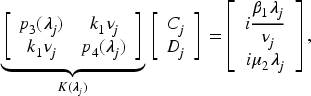
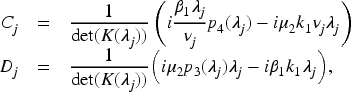
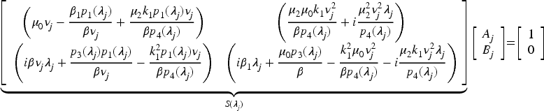
depend on

λ

and will be determined explicitly in the sequel. System (41) is equivalent to

\begin{array}{rcl} p_{1} (λ) A_{j} + μ_{0} ν_{j} B_{j} - β ν_{j} C_{j} & = & r_{1}, \\ μ_{0} ν_{j} A_{j} + p_{2} (λ) B_{j} - β_{1} C_{j} - μ_{2} ν_{j} D_{j} & = & r_{2}, \\ i β λ ν_{j} A_{j} + i λ β_{1} B_{j} + p_{3} (λ) C_{j} + k_{1} ν_{j} D_{j} & = & r_{3}, \\ i μ_{2} λ ν_{j} B_{j} + k_{1} ν_{j} C_{j} + p_{4} (λ) D_{j} & = & 0, \end{array}

(42)

where

\begin{array}{rcl} p_{1} (λ) & := & - λ^{2} ρ + μ ν_{j}^{2} \\ p_{2} (λ) & := & - λ^{2} J + a_{0} ν_{j} + ξ \\ p_{3} (λ) & := & i λ c + k ν_{j} \\ p_{4} (λ) & := & i λ b + k_{6} ν_{j}^{2} + k_{2} . \end{array}

(43)

Let us analyse the algebraic systems (42) and (43) by cases.

(I) Case $β = 0$ . In this case we have two situations associated to $μ_{0}$ .

Sub-case $μ_{0} = 0$ . In this case, the first equation of (1) reduces to an uncoupled plate equation with oscillatory solutions. So the whole system is not asymptomatically stable.

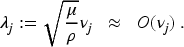
Sub-case $μ_{0} \neq 0$ . In this case, we consider in system (42), $r_{1} = - μ_{0}$ , $r_{2} = r_{3} = 0$ and, for $j$ large enough, $λ_{j}$ as a positive root of $p_{1} (λ) = 0$ . This is, we define $λ_{j}$ as

λ_{j} := \sqrt{\frac{μ}{ρ}} ν_{j} \approx O (ν_{j}) .

Consequently, from the first equation of (42), we obtain

B_{j} = - 1 / ν_{j}

, for all

j \in N

. So substituting in the third and fourth equations of (42), using that

β = 0

, we obtain the system

\underset{K (λ_{j})}{\underset{⏟}{[\begin{array}{cc} p_{3} (λ_{j}) & k_{1} ν_{j} \\ k_{1} ν_{j} & p_{4} (λ_{j}) \end{array}]}} [\begin{matrix} C_{j} \\ D_{j} \end{matrix}] = [\begin{matrix} i \frac{β_{1} λ_{j}}{ν_{j}} \\ i μ_{2} λ_{j} \end{matrix}],

where, from (43), we have

det (K (λ_{j})) = p_{3} (λ_{j}) p_{4} (λ_{j}) - k_{1}^{2} ν_{j}^{2} := p_{5} (λ_{j}) + i p_{6} (λ_{j})

where, using the definition of

λ_{j}

\begin{array}{rcl} p_{5} (λ) & := & k_{6} k ν_{j}^{3} - (\frac{c b μ}{ρ} + k_{1}^{2}) ν_{j}^{2} + k_{2} k ν_{j} \approx O (ν_{j}^{3}), \\ p_{6} (λ) & := & k_{6} c \sqrt{\frac{μ}{ρ}} ν_{j}^{3} + b ρ k \sqrt{\frac{μ}{ρ}} ν_{j}^{2} + c k_{2} \sqrt{\frac{μ}{ρ}} ν_{j} \approx O (ν_{j}^{3}) . \end{array}

(44)

Solving the previous matrix system by Cramer’s rule, we obtain

C_{j} = \frac{det [\begin{array}{cc} i \frac{β_{1} λ_{j}}{ν_{j}} & k_{1} ν_{j} \\ i μ_{2} λ_{j} & p_{4} (λ_{j}) \end{array}]}{det (K (λ_{j}))} and D_{j} = \frac{det [\begin{array}{cc} p_{3} (λ_{j}) & i \frac{β_{1} λ_{j}}{ν_{j}} \\ k_{1} ν_{j} & i μ_{2} λ_{j} \end{array}]}{det (K (λ_{j}))},

this is

\begin{array}{rcl} C_{j} & = & \frac{1}{det (K (λ_{j}))} (i \frac{β_{1} λ_{j}}{ν_{j}} p_{4} (λ_{j}) - i μ_{2} k_{1} ν_{j} λ_{j}) \\ D_{j} & = & \frac{1}{det (K (λ_{j}))} (i μ_{2} p_{3} (λ_{j}) λ_{j} - i β_{1} k_{1} λ_{j}), \end{array}

where, using again (43) and definition of

λ_{j}

\begin{array}{rcl} C_{j} & = & \frac{1}{det (K (λ_{j}))} [\frac{- β_{1} μ b}{ρ} ν_{j} + i ((β_{1} k_{6} - k_{1} μ_{2}) \sqrt{\frac{μ}{ρ}} ν_{j}^{2} + β_{1} k_{2} \sqrt{\frac{μ}{ρ}})], \\ D_{j} & = & \frac{1}{det (K (λ_{j}))} [- \frac{μ μ_{2} c}{ρ} ν_{j}^{2} + i \sqrt{\frac{μ}{ρ}} (k μ_{2} ν_{j}^{2} - β_{1} k_{1} ν_{j})] . \end{array}

(45)

Finally, from the second equation of (42), using that

B_{j} = - 1 / ν_{j}

, we obtain

A_{j} = \frac{p_{2} (λ_{j})}{μ_{0} ν_{j}^{2}} + (\frac{β_{1}}{μ_{0} ν_{j}} C_{j} + \frac{μ_{2}}{μ_{0}} D_{j}) .

Then, using (45), we deduce that

A_{j} = \frac{p_{2} (λ_{j})}{μ_{0} ν_{j}^{2}} + \frac{1}{det (K (λ_{j}))} [p_{7} (λ_{j}) + i p_{8} (λ_{j})],

where

\begin{array}{rcl} p_{7} (λ) & := & - \frac{μ_{2}^{2} μ c}{μ_{0} ρ} ν_{j}^{2} - \frac{β_{1}^{2} μ b}{μ_{0} ρ} \approx O (ν_{j}^{2}), \\ p_{8} (λ) & := & \sqrt{\frac{μ}{ρ}} \frac{k μ_{2}^{2}}{μ_{0}} ν_{j}^{2} + ((β_{1} k_{6} - k_{1} μ_{2}) \frac{β_{1}}{μ_{0}} \sqrt{\frac{μ}{ρ}} - \frac{μ_{2} β_{1} k_{1}}{μ_{0}}) ν_{j} + \frac{β_{1}^{2} k_{2}}{μ_{0} ν_{j}} \sqrt{\frac{μ}{ρ}} . \end{array}

(46)

Then, using (43), (44) and (46) we deduce that

| A_{j} | = \frac{| [p_{2} (λ_{j}) p_{5} (λ_{j}) + μ_{0} ν_{j}^{2} p_{7} (λ_{j})] + i [p_{2} (λ_{j}) p_{6} (λ_{j}) + μ_{0} ν_{j}^{2} p_{8} (λ_{j})] |}{| [μ_{0} ν_{j}^{2} p_{5} (λ_{j})] + i [μ_{0} ν_{j}^{2} p_{6} (λ_{j})] |} \approx \frac{O (ν_{j}^{5})}{O (ν_{j}^{5})} .

Taking into account (43), (44) and (46), we get

| | U_{j} | |_{H} \geq C | | Δ u_{j} | |_{L^{2}} = C | | ν_{j} A_{j} e_{j} | |_{L^{2}} = C ν_{j} | A_{j} | \approx O (ν_{j}) ⟶ \infty,

where

| | e_{j} | |_{L^{2}} = 1

, for all

j \in N

. This implies that, in the case

β = 0

with

μ_{0} \neq 0

, the system is also not exponentially stable.

Before the analysis of the case $μ_{2} = 0$ , we reformulate system (42) assuming now $β \neq 0$ and taking $r_{1} = 0$ . Then, from equations (42) $_{1}$ and (42) $_{4}$ , we obtain

C_{j} = \frac{p_{1} (λ)}{β ν_{j}} A_{j} + \frac{μ_{0}}{β} B and D_{j} = - \frac{k_{1} p_{1} (λ)}{β p_{4} (λ)} A_{j} - (\frac{μ_{0} k_{1}}{β} ν_{j} + i \frac{μ_{2} ν_{j} λ}{p_{4} (λ)}) B_{j},

and substituting into (42)

_{2}

and (42)

_{3}

, we have

\underset{S (λ)}{\underset{⏟}{[\begin{array}{cc} (μ_{0} ν_{j} - \frac{β_{1} p_{1} (λ)}{β ν_{j}} + \frac{μ_{2} k_{1} p_{1} (λ) ν_{j}}{β p_{4} (λ)}) & (p_{2} (λ) - \frac{β_{1} μ_{0}}{β} + \frac{μ_{2} μ_{0} k_{1} ν_{j}^{2}}{β p_{4} (λ)} + i \frac{μ_{2}^{2} ν_{j}^{2} λ}{p_{4} (λ)}) \\ (i β ν_{j} λ + \frac{p_{3} (λ) p_{1} (λ)}{β ν_{j}} - \frac{k_{1}^{2} p_{1} (λ) ν_{j}}{β p_{4} (λ)}) & (i β_{1} λ + \frac{μ_{0} p_{3} (λ)}{β} - \frac{k_{1}^{2} μ_{0} ν_{j}^{2}}{β p_{4} (λ)} - i \frac{μ_{2} k_{1} ν_{j}^{2} λ}{p_{4} (λ)}) \end{array}]}} [\begin{matrix} A_{j} \\ B_{j} \end{matrix}] = [\begin{matrix} r_{2} \\ r_{3} \end{matrix}]

(47)

(II) Case

μ_{2} = 0

. In this situation, (47) becomes to

\underset{T (λ)}{\underset{⏟}{[\begin{array}{cc} (μ_{0} ν_{j} - \frac{β_{1} p_{1} (λ)}{β ν_{j}}) & (p_{2} (λ) - \frac{β_{1} μ_{0}}{β}) \\ (i β ν_{j} λ + \frac{p_{3} (λ) p_{1} (λ)}{β ν_{j}} - \frac{k_{1}^{2} p_{1} (λ) ν_{j}}{β p_{4} (λ)}) & (i β_{1} λ + \frac{μ_{0} p_{3} (λ)}{β} - \frac{k_{1}^{2} μ_{0} ν_{j}^{2}}{β p_{4} (λ)}) \end{array}]}} [\begin{matrix} A_{j} \\ B_{j} \end{matrix}] = [\begin{matrix} r_{2} \\ r_{3} \end{matrix}]

(48)

So, even in the case

μ_{2} = 0

we have different situations depending of

μ_{0}

and

β_{1}

. We divide this analysis in sub-cases.

Sub-case $μ_{0} = β_{1} = 0$ . In this case, the second equation of (1) reduces to an uncoupled wave equation with oscillatory solutions which turns the system non-asymptotically stable. In fact, here we can choose $r_{2} = 1$ and, for $j$ large enough, $λ_{j}$ as a positive root of $p_{2} (λ) = 1$ . This is, we define $λ_{j}$ by

λ_{j} := \sqrt{\frac{a_{0} ν_{j} + ξ - 1}{J}} \approx O (ν_{j}^{1 / 2}) .

So, from (48)

_{1}

, we obtain

B_{j} = 1

, for all

j \in N

. Then, using that

φ_{j} = B_{j} e_{j}

, we obtain

| | U_{j} | |_{H} \geq \sqrt{a_{0}} | | \nabla φ_{j} | |_{L^{2}} = \sqrt{a_{0}} | | ν_{j}^{1 / 2} B_{j} e_{j} | |_{L^{2}} = \sqrt{a_{0}} ν_{j}^{1 / 2} \approx O (ν_{j}^{1 / 2}) ⟶ \infty,

(49)

This implies that, in the case

μ_{2} = 0

with

μ_{0} = β_{1} = 0

, the system is not exponentially stable.

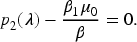
Sub-case $μ_{0} \neq 0$ or $β_{1} \neq 0$ . In this case, for $j$ large enough, we define $λ_{j}$ as a positive root of

p_{2} (λ) - \frac{β_{1} μ_{0}}{β} = 0.

This is

λ_{j} := \sqrt{\frac{a_{0} ν_{j} + ξ β - β_{1} μ_{0}}{β J}} \approx O (ν_{j}^{1 / 2}) .

(50)

So, considering

r_{2} = 1

and

r_{3} = 0

, the previous system is rewritten as

\underset{T (λ_{j})}{\underset{⏟}{[\begin{array}{cc} (μ_{0} ν_{j} - \frac{β_{1} p_{1} (λ_{j})}{β ν_{j}}) & 0 \\ (i β ν_{j} λ_{j} + \frac{p_{3} (λ_{j}) p_{1} (λ_{j})}{β ν_{j}} - \frac{k_{1}^{2} p_{1} (λ_{j}) ν_{j}}{β p_{4} (λ_{j})}) & (i β_{1} λ_{j} + \frac{μ_{0} p_{3} (λ_{j})}{β} - \frac{k_{1}^{2} μ_{0} ν_{j}^{2}}{β p_{4} (λ_{j})}) \end{array}]}} [\begin{matrix} A_{j} \\ B_{j} \end{matrix}] = [\begin{matrix} 1 \\ 0 \end{matrix}] .

Then, using the definition of

p_{1} (λ)

given by (43)

_{1}

, we obtain

\begin{array}{rcl} det (T (λ_{j})) & = & (μ_{0} ν_{j} - \frac{β_{1} p_{1} (λ_{j})}{β ν_{j}}) (i β_{1} λ_{j} + \frac{μ_{0} p_{3} (λ_{j})}{β} - \frac{k_{1}^{2} μ_{0} ν_{j}^{2}}{β p_{4} (λ_{j})}) \\ = & \frac{1}{β^{2} ν_{j} [p_{4} (λ_{j})]^{2}} T_{1} (λ_{j}) T_{2} (λ_{j}), \end{array}

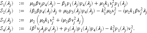
where

\begin{array}{rcl} T_{1} (λ_{j}) & := & (μ_{0} - β_{1} μ) ν_{j}^{2} + β_{1} ρ λ_{j}^{2} \\ T_{2} (λ_{j}) & := & i β_{1} β p_{4} (λ_{j}) λ_{j} + μ_{0} p_{3} (λ_{j}) p_{4} (λ_{j}) - k_{1}^{2} μ_{0} ν_{j}^{2} . \end{array}

Here, using (50), in general when

μ_{0} - β_{1} μ \neq 0

, the order

O (T_{1} (λ_{j}))

is given by

O (ν_{j}^{2})

. On the other hand, the higher order term of

T_{2} (λ_{j})

is associated to the order of the term

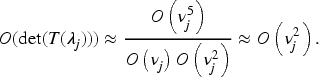
O (T_{2} (λ_{j})) = O (μ_{0} p_{3} (λ_{j}) p_{4} (λ_{j})) = O (μ_{0} k k_{6} ν_{j}^{3}) \approx O (ν_{j}^{3}) .

Note that it is depends of

μ_{0} \neq 0

. Otherwise the order

O (T_{2} (λ_{j}))

is given by

O (ν_{j}^{2 + 1 / 2})

, which is associated to the term

i β_{1} β p_{4} (λ_{j}) λ_{j}

. So, from the previous analysis we can conclude that, at maximum, the order of

det (T (λ_{j}))

is given by

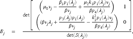
O (det (T (λ_{j}))) \approx \frac{O (ν_{j}^{5})}{O (ν_{j}) O (ν_{j}^{2})} \approx O (ν_{j}^{2}) .

So, solving the previous system by Cramer’s rule, we obtain

B_{j} = \frac{det [\begin{array}{cc} (μ_{0} ν_{j} - \frac{β_{1} p_{1} (λ_{j})}{β ν_{j}}) & 1 \\ (i β ν_{j} λ_{j} + \frac{p_{3} (λ_{j}) p_{1} (λ_{j})}{β ν_{j}} - \frac{k_{1}^{2} p_{1} (λ_{j}) ν_{j}}{β p_{4} (λ_{j})}) & 0 \end{array}]}{det (T (λ_{j}))},

this is

B_{j} = \frac{i β^{2} ν_{j}^{2} λ_{j} p_{4} (λ_{j}) + p_{3} (λ_{j}) p_{1} (λ_{j}) p_{4} (λ_{j}) - k_{1}^{2} ν_{j}^{2} p_{1} (λ_{j})}{β ν_{j} p_{4} (λ_{j}) det (T (λ_{j}))} .

(51)

Here, note that the higher order term of the numerator of

B_{j}

is given by

Re (p_{3} (λ_{j}) p_{1} (λ_{j}) p_{4} (λ_{j}))

, because it is exactly associated to the positive term

μ k k_{6} ν_{j}^{5}

, which means, using (43) and (50), that

O (Re (p_{3} (λ_{j}) p_{1} (λ_{j}) p_{4} (λ_{j}))) \approx O (μ k k_{6} ν_{j}^{5}) \approx O (ν_{j}^{5}) .

(52)

So, in the extremal case, using (40) we have in (51) that

| B_{j} | \approx \frac{O (ν_{j}^{5})}{O (ν_{j}) O (ν_{j}^{2}) O (ν_{j}^{2})} \approx \frac{O (ν_{j}^{5})}{O (ν_{j}^{5})},

which implies, using similar argument used to obtain (49), that the system is not exponentially stable.

Remark 5.1

Note that the previous analysis is independent of $k_{1} \in R$ .

5.2. Lack of Differentiability

Finally, we will show that, in the presence of the terms $μ_{2} \neq 0$ and $β \neq 0$ , there is no gain of regularity for the solutions of the system. This is, the semigroup associated to the system is not differentiable (Pazy, 1983) (non-immediately differentiable; Engel & Nagel, 2000). For this purpose, we will use the following result:

Theorem 5.2
Let $A$ the infinitesimal generator of an immediately norm continuous exponentially stable semigroup. Then
$lim_{| λ | \to \infty} | | (i λ I - A)^{- 1} | | = 0.$

Proof.
Engel and Nagel (2000, Corollary 4.19, pg.114).
Remark 5.3
Note that in Section 4, we already proved that the semigroup is exponentially stable when $μ_{2} \neq 0$ and $β \neq 0$ . As follows, using the previous theorem, we will prove that the same semigroup is not immediately norm continuous, which implies no immediate differentiability.

In fact, based in Theorem 5.2, it is sufficient to prove that there exists a sequence ${F_{j}}_{j \in N} \subset H$ (bounded), and ${λ_{j}}_{j \in N} \subset R^{+}$ with $lim_{j \to \infty} λ_{j} = \infty$ , such that $U_{j}$ is the solution of the resolvent system (40), satisfying
$lim_{j \to \infty} | | U_{j} | |_{H} > 0.$
Taking advantage of the construction made in the previous Section 5.1, we use the sequence $(λ_{j})$ given by (50), which satisfies $p_{2} (λ_{j}) - (β_{1} μ_{0} / β) = 0$ . Then, using into system (47) with $r_{2} = 1$ and $r_{3} = 0$ , we have the system
$\underset{S (λ_{j})}{\underset{⏟}{[\begin{array}{cc} (μ_{0} ν_{j} - \frac{β_{1} p_{1} (λ_{j})}{β ν_{j}} + \frac{μ_{2} k_{1} p_{1} (λ_{j}) ν_{j}}{β p_{4} (λ_{j})}) & (\frac{μ_{2} μ_{0} k_{1} ν_{j}^{2}}{β p_{4} (λ_{j})} + i \frac{μ_{2}^{2} ν_{j}^{2} λ_{j}}{p_{4} (λ_{j})}) \\ (i β ν_{j} λ_{j} + \frac{p_{3} (λ_{j}) p_{1} (λ_{j})}{β ν_{j}} - \frac{k_{1}^{2} p_{1} (λ_{j}) ν_{j}}{β p_{4} (λ_{j})}) & (i β_{1} λ_{j} + \frac{μ_{0} p_{3} (λ_{j})}{β} - \frac{k_{1}^{2} μ_{0} ν_{j}^{2}}{β p_{4} (λ_{j})} - i \frac{μ_{2} k_{1} ν_{j}^{2} λ_{j}}{p_{4} (λ_{j})}) \end{array}]}} [\begin{matrix} A_{j} \\ B_{j} \end{matrix}] = [\begin{matrix} 1 \\ 0 \end{matrix}]$
where
$\begin{array}{rcl} det (S (λ_{j})) & = & (μ_{0} ν_{j} - \frac{β_{1} p_{1} (λ_{j})}{β ν_{j}} + \frac{μ_{2} k_{1} p_{1} (λ_{j}) ν_{j}}{β p_{4} (λ_{j})}) (i β_{1} λ_{j} + \frac{μ_{0} p_{3} (λ_{j})}{β} - \frac{k_{1}^{2} μ_{0} ν_{j}^{2}}{β p_{4} (λ_{j})} - i \frac{μ_{2} k_{1} ν_{j}^{2} λ_{j}}{p_{4} (λ_{j})}) \\ - (\frac{μ_{2} μ_{0} k_{1} ν_{j}^{2}}{β p_{4} (λ_{j})} + i \frac{μ_{2}^{2} ν_{j}^{2} λ_{j}}{p_{4} (λ_{j})}) (i β ν_{j} λ_{j} + \frac{p_{3} (λ_{j}) p_{1} (λ_{j})}{β ν_{j}} - \frac{k_{1}^{2} p_{1} (λ_{j}) ν_{j}}{β p_{4} (λ_{j})}) \\ = & \frac{1}{β^{2} ν_{j} [p_{4} (λ_{j})]^{2}} [S_{1} (λ_{j}) S_{2} (λ_{j}) - S_{3} (λ_{j}) S_{4} (λ_{j})], \end{array}$
where
$\begin{array}{rcl} S_{1} (λ_{j}) & := & μ_{0} β ν_{j} p_{4} (λ_{j}) - β_{1} p_{1} (λ_{j}) p_{4} (λ_{j}) + μ_{2} k_{1} ν_{j}^{2} p_{1} (λ_{j}) \\ S_{2} (λ_{j}) & := & i β_{1} β p_{4} (λ_{j}) λ_{j} + μ_{0} p_{3} (λ_{j}) p_{4} (λ_{j}) - k_{1}^{2} μ_{0} ν_{j}^{2} - i μ_{2} k_{1} β ν_{j}^{2} λ_{j} \\ S_{3} (λ_{j}) & := & μ_{2} (μ_{0} k_{1} ν_{j}^{2} + i μ_{2} β ν_{j}^{2} λ_{j}) \\ S_{4} (λ_{j}) & := & i β^{2} ν_{j} λ_{j} p_{4} (λ_{j}) + p_{3} (λ_{j}) p_{1} (λ_{j}) p_{4} (λ_{j}) - k_{1}^{2} p_{1} (λ_{j}) ν_{j}^{2} . \end{array}$
Here, note that the higher order term of the numerator of $det (S (λ_{j}))$ is associated to the term $S_{3} (λ_{j}) S_{4} (λ_{j})$ . More specifically, it is associated to the term
$i μ_{2}^{2} β ν_{j}^{2} λ_{j} p_{3} (λ_{j}) p_{1} (λ_{j}) p_{4} (λ_{j}) .$
Therefore, using (43), (50) and (52) we see that
$\begin{array}{rcl} det (S (λ_{j})) & = & \frac{i μ_{2}^{2} β ν_{j}^{2} \sqrt{\frac{a_{0} ν_{j} + ξ β - β_{1} μ_{0}}{J}} μ k k_{6} ν_{j}^{5} + \dots `` low order terms'' \dots}{β^{2} ν_{j} {[i λ_{j} b + k_{6} ν_{j}^{2} + k_{2}]}^{2}}, \end{array}$
this is
$det (S (λ_{j})) = \frac{i μ_{2}^{2} μ β k k_{6} \sqrt{\frac{a_{0}}{J}} ν_{j}^{7 + 1 / 2} + \dots `` l.o.t.'' \dots}{β^{2} ν_{j} {[i λ_{j} b + k_{6} ν_{j}^{2} + k_{2}]}^{2}} .$
(53)
So, calculating $B_{j}$ we obtain
$B_{j} = \frac{det [\begin{array}{cc} (μ_{0} ν_{j} - \frac{β_{1} p_{1} (λ_{j})}{β ν_{j}} + \frac{μ_{2} k_{1} p_{1} (λ_{j}) ν_{j}}{β p_{4} (λ_{j})}) & 1 \\ (i β ν_{j} λ_{j} + \frac{p_{3} (λ_{j}) p_{1} (λ_{j})}{β ν_{j}} - \frac{k_{1}^{2} p_{1} (λ_{j}) ν_{j}}{β p_{4} (λ_{j})}) & 0 \end{array}]}{det (S (λ_{j}))},$
this is
$\begin{aligned} B_{j} = \frac{i β^{2} ν_{j}^{2} λ_{j} p_{4} (λ_{j}) + p_{3} (λ_{j}) p_{1} (λ_{j}) p_{4} (λ_{j}) - k_{1} p_{1} (λ_{j}) ν_{j}^{2}}{β ν_{j} p_{4} (λ_{j}) det (S (λ_{j}))} . \end{aligned}$
Here again, the higher order term of the numerator of $B_{j}$ is associated to
$O (p_{3} (λ_{j}) p_{1} (λ_{j}) p_{4} (λ_{j})) \approx O (μ k k_{6} ν_{j}^{5}) .$
Then, from (53), we deduce
$\begin{array}{rcl} B_{j} & = & \frac{β [i λ_{j} b + k_{6} ν_{j}^{2} + k_{2}] (μ k k_{6} ν_{j}^{5} + \dots `` l.o.t.'' \dots)}{i μ_{2}^{2} μ β k k_{6} \sqrt{\frac{a_{0}}{J}} ν_{j}^{7 + 1 / 2} + \dots `` l.o.t.'' \dots} = \frac{k_{6} ν_{j}^{7} + \dots `` l.o.t.'' \dots}{i μ_{2}^{2} \sqrt{\frac{a_{0}}{J}} ν_{j}^{7 + 1 / 2} + \dots `` l.o.t.'' \dots} . \end{array}$
Therefore, based on the arguments used in (49) we can conclude that
$lim_{j \to \infty} ‖ U_{j} ‖_{H} \geq lim_{j \to \infty} \sqrt{a_{0}} ‖ ν_{j}^{1 / 2} B_{j} e_{j} ‖ = \frac{k_{6} \sqrt{J}}{μ_{2}^{2}} > 0,$
which implies $lim_{| λ | \to \infty} | | (i λ I - A)^{- 1} | | > 0$ . So, our conclusion follows from Theorem 5.2 and Remark 5.3.
6. Polynomial Decay Rates

In this section we obtain certain polynomial decay rates for the cases $β = 0$ and/or $μ_{2} = 0$ . For each case we will take advantage of results obtained in Section 4. The results of well-posedness obtained in Section 3 are still valid for these situations. For this purpose, we will use the following characterisation:

Theorem 6.1
Let ${e^{t A}}_{t \geq 0}$ be a bounded $C_{0}$ -semigroup on a Hilbert space $H$ such that $i R \subset ϱ (A)$ . For a fixed $r > 0$ , the following conditions are equivalent: (a)
There exists $λ_{0} > 0$ such that
$| | (i λ I - A)^{- 1} | |_{L (H)} \leq O (| λ |^{r}), \forall | λ | \geq λ_{0} .$

(b)
There exists $t_{0} > 0$ such that
$| | e^{t A} A^{- 1} | |_{L (H)} \leq O (t^{- 1 / r}), \forall t \geq t_{0} .$

Proof.
Direct consequence of Theorem 2.4 in Borichev and Tomilov (2010).

We start analysing the extremal case where $β = μ_{2} = 0$ . The other situations will be quite similar.
6.1. Case $β = μ_{2} = 0$

Here the associated system is

\begin{array}{rcl} ρ u_{t t} + μ Δ^{2} u - μ_{0} Δ φ & = & 0, \\ J φ_{t t} - a_{0} Δ φ + ξ φ - μ_{0} Δ u - β_{1} θ & = & 0, \\ c θ_{t} - k Δ θ - k_{1} Δ T + β_{1} φ_{t} & = & 0, \\ b T_{t} + k_{6} Δ^{2} T + k_{2} T - k_{1} Δ θ & = & 0, \end{array}

(54)

with the corresponding boundary and initial conditions given by (2) and (3). Note that, necessarily,

β_{1} \neq 0 and μ_{0} \neq 0.

Otherwise we are working with an uncoupled system with periodic solutions.

In this case the proof of $i R \subset ϱ (A)$ follows similar arguments proposed by equations (11) and (12), with the difference that systems (13)–(18) is reduced to

\begin{aligned} i ω_{n} u_{n} - v_{n} \to & 0 in H^{2} (Ω) \cap H_{0}^{1} (Ω) \end{aligned}

(55)

\begin{aligned} i ω_{n} ρ v_{n} + μ Δ^{2} u_{n} - μ_{0} Δ φ_{n} \to & 0 in L^{2} (Ω) \end{aligned}

(56)

\begin{aligned} i ω_{n} φ_{n} - ψ_{n} \to & 0 in H_{0}^{1} (Ω) \end{aligned}

(57)

\begin{aligned} i ω_{n} J ψ_{n} - a_{0} Δ φ_{n} + ξ φ_{n} - μ_{0} Δ u_{n} - β_{1} θ_{n} \to & 0 in L^{2} (Ω) \end{aligned}

(58)

\begin{aligned} i ω_{n} c θ_{n} - k Δ θ_{n} - k_{1} Δ T_{n} + β_{1} ψ_{n} \to & 0 in L^{2} (Ω) \end{aligned}

(59)

\begin{aligned} i ω_{n} b T_{n} + k_{6} Δ^{2} T_{n} + k_{2} T_{n} - k_{1} Δ θ_{n} \to & 0 in L^{2} (Ω) . \end{aligned}

(60)

Here, the calculations used to obtain (21) are still valid. This is

θ_{n} ⟶ 0 in H_{0}^{1} (Ω) and T_{n} ⟶ 0 in H^{2} (Ω) \cap H_{0}^{1} (Ω) .

(61)

To obtain (22) it was used condition

μ_{2} \neq 0

. In this case, taking into account that

β_{1} \neq 0

, we multiply (59) by

ψ_{n} \in L^{2}

and, using (61), we obtain

- k (Δ θ_{n}, ψ_{n})_{L^{2}} + β_{1} | | ψ_{n} | |^{2} \to 0.

Additionally, from (57) we can deduce, using (61) again, that

(\nabla θ_{n}, \nabla ψ_{n})_{L^{2}} \to 0

. So, combining these convergences, (22) is still valid. This is

ψ_{n} ⟶ 0 in L^{2} (Ω) .

(62)

This implies, by (57), that (23) holds. This is

φ_{n} ⟶ 0 in L^{2} (Ω) .

(63)

So, similarly to the procedure to obtain (27), using (61), (62) and (63), we obtain

φ_{n} ⟶ 0 in H_{0}^{1} (Ω) .

(64)

Now, multiplying (58) by

z_{n}

L^{2}

, where

z_{n}

is given by (24), we obtain

i ω_{n} J (ψ_{n}, z_{n})_{L^{2}} + a_{0} (φ_{n}, v_{n})_{L^{2}} + ξ (φ_{n}, z_{n})_{L^{2}} + μ_{0} (u_{n}, v_{n})_{L^{2}} - β_{1} (θ_{n}, z_{n})_{L^{2}} ⟶ 0.

So, using (61), (62) and (63), we get

μ_{0} (u_{n}, v_{n})_{L^{2}} ⟶ 0.

(65)

So, multiplying (56) by

u

L^{2}

, using (63) and (65), we obtain

u_{n} ⟶ 0 in H^{2} (Ω) \cap H_{0}^{1} (Ω),

(66)

which also implies, by (55), that

v_{n} ⟶ 0 in L^{2} (Ω) .

(67)

Therefore, combining (61), (62), (64), (66) and (67) we obtain

U_{n} ⟶ 0 in H,

which is a contradiction with

| | U_{n} | |_{H} = 1

given by (11). Consequently, condition (9) holds.

On the other hand, in order to prove condition (a) of Theorem 6.1, note that the resolvent equation (28) is reduced to

\begin{aligned} i λ u - v = & f_{1} in H^{2} (Ω) \cap H_{0}^{1} (Ω) \end{aligned}

(68)

\begin{aligned} i λ ρ v + μ Δ^{2} u - μ_{0} Δ φ = & ρ f_{2} in L^{2} (Ω) \end{aligned}

(69)

\begin{aligned} i λ φ - ψ = & f_{3} in H_{0}^{1} (Ω) \end{aligned}

(70)

\begin{aligned} i λ J ψ - a_{0} Δ φ + ξ φ - μ_{0} Δ u - β_{1} θ = & J f_{4} in L^{2} (Ω) \end{aligned}

(71)

\begin{aligned} i λ c θ - k Δ θ - k_{1} Δ T + β_{1} ψ = & c f_{5} in L^{2} (Ω) \end{aligned}

(72)

\begin{aligned} i λ b T + k_{6} Δ^{2} T + k_{2} T - k_{1} Δ θ = & b f_{6} in L^{2} (Ω) . \end{aligned}

(73)

Here, it is not difficult to see that Lemma 4.2 is still valid. On the other hand, Lemma 4.3 will be replaced by the following:

Lemma 6.2

For all $U = (u, v, φ, ψ, θ, T)^{'} \in D (A)$ , there exists a positive constant $C$ , being independent of $F$ such that

| | ψ | |_{L^{2}}^{2} \leq C | λ | | | U | |_{H} | | \nabla θ | |_{L^{2}} + C | | U | |_{H} | | F | |_{H} + C | | F | |_{H}^{2} .

Proof.

Multiplying (72) by $ψ \in L^{2}$ , we obtain

β_{1} | | ψ | |_{L^{2}}^{2} = - i λ c (θ, ψ)_{L^{2}} + \underset{J_{1}}{\underset{⏟}{(Δ θ, ψ)_{L^{2}}}} - k_{1} (Δ T, ψ)_{L^{2}} + c (f_{5}, ψ)_{L^{2}},

where, from (70) and Lemma 4.2, we deduce

\begin{array}{rcl} | J_{1} | & = & | i λ k (\nabla θ, \nabla φ)_{L^{2}} + k (\nabla θ, \nabla f_{3})_{L^{2}} | \\ \leq & C | λ | | | \nabla θ | |_{L^{2}} | | \nabla φ | |_{L^{2}} + C | | \nabla θ | |_{L^{2}} | | \nabla f_{3} | |_{L^{2}} \\ \leq & C | λ | | | \nabla θ | |_{L^{2}} | | U | |_{H} + C | | U | |_{H} | | F | |_{H} + C | | F | |_{H}^{2} . \end{array}

Therefore, using this estimative in the previous equality, noting that

β_{1} \neq 0

, the results follows.

Now, in order to estimate $v$ , we replace Lemma 4.5 by the following:

Lemma 6.3

Using the same hypotheses as in Lemma 6.2, for $| λ |$ large enough, there exists $C > 0$ such that

| | v | |_{L^{2}}^{2} \leq C | λ |^{2} | | ψ | |_{L^{2}} | | v | |_{L^{2}} + | λ | | | U | |_{H} | | F | |_{H} + | λ | | | U | |_{H} | | \nabla θ | |_{L^{2}} .

(74)

Proof.

Multiplying (71) by $i λ z$ in $L^{2}$ , where $z$ is given in (35), we obtain

μ_{0} | | v | |_{L^{2}}^{2} = λ^{2} J (ψ, z)_{L^{2}} \underset{J_{2}}{\underset{⏟}{- i λ a_{0} (φ, v)_{L^{2}} - i λ ξ (φ, z)_{L^{2}}}} + i λ β_{1} (θ, z)_{L^{2}} - i λ J (f_{4}, z)_{L^{2}},

where using (70), we deduce

| J_{2} | = d | (i λ φ, a_{0} v + ξ z)_{L^{2}} | = | (ψ + f_{3}, a_{0} v + ξ z)_{L^{2}} | \leq C | | ψ | |_{L^{2}} | | v | |_{L^{2}} + | | | U | |_{H} | | F | |_{H} .

So, substituting this estimative in the previous equality, using Lemma 4.2 and noting that

μ_{0} \neq 0

, the results follows.

Additionally, we establish the following estimative:

Lemma 6.4

Under the same assumptions as in Lemma 6.2, for $| λ |$ large enough, there exists $C > 0$ such that

| | Δ u | |_{L^{2}}^{2} + | | \nabla φ | |_{L^{2}}^{2} \leq ρ | | v | |_{L^{2}}^{2} + J | | ψ | |_{L^{2}}^{2} + C | | U | |_{H} | | F | |_{H} .

(75)

Proof.

Multiplying (69) by $u$ and (71) by $φ$ in $L^{2}$ , using Lemma 4.2, the results follows without difficulties.

Finally, doing $2 ρ$ (74)+(75), we obtain

ρ | | v | |_{L^{2}}^{2} + | | Δ u | |_{L^{2}}^{2} + | | \nabla φ | |_{L^{2}}^{2} \leq C | λ |^{2} | | ψ | |_{L^{2}} | | v | |_{L^{2}} + J | | ψ | |_{L^{2}}^{2} + C | λ | | | U | |_{H} | | F | |_{H} + C | | U | |_{H} | | \nabla θ | |_{L^{2}},

which implies, taking

| λ |

large enough and using Lemma 6.2, that

\begin{array}{rcl} \frac{ρ}{2} | | v | |_{L^{2}}^{2} + | | Δ u | |_{L^{2}}^{2} + | | \nabla φ | |_{L^{2}}^{2} & \leq & C | λ |^{4} | | ψ | |_{L^{2}}^{2} + C | λ | | | U | |_{H} | | F | |_{H} + C | | U | |_{H} | | \nabla θ | |_{L^{2}} \\ \leq & C | λ |^{4} (| λ | | | U | |_{H} | | \nabla θ | |_{L^{2}} + | | U | |_{H} | | F | |_{H} + | | F | |_{H}^{2}) \\ + C | λ | | | U | |_{H} | | F | |_{H} + C | | U | |_{H} | | \nabla θ | |_{L^{2}}, \end{array}

this is

\frac{ρ}{2} | | v | |_{L^{2}}^{2} + | | Δ u | |_{L^{2}}^{2} + | | \nabla φ | |_{L^{2}}^{2} \leq C | λ |^{5} (| | U | |_{H} | | \nabla θ | |_{L^{2}} + | | U | |_{H} | | F | |_{H}) + C | λ |^{4} | | F | |_{H}^{2} .

Here, after again Lemmas 4.2 and 6.2, we get

\frac{ρ}{2} | | v | |_{L^{2}}^{2} + | | Δ u | |_{L^{2}}^{2} + | | \nabla φ | |_{L^{2}}^{2} + | | ψ | |_{L^{2}}^{2} \leq C | λ |^{5} (| | U | |_{H} | | \nabla θ | |_{L^{2}} + | | U | |_{H} | | F | |_{H}) + C | λ |^{4} | | F | |_{H}^{2} .

Therefore, combining the previous estimative with 4.2, we obtain, for

λ

large enough,

| | U | |_{H}^{2} \leq C | λ |^{10} | | U | |_{H} | | F | |_{H} + C | λ |^{4} | | F | |_{H}^{2},

implying

| | U | |_{L^{2}} \leq C | λ |^{10} | | F | |_{H}, for all | λ | large enough .

Consequently, condition (a) of Theorem 6.1 holds for

r = 10

. This implies polynomial stability of the solutions of the system in the case

β = μ_{2} = 0

6.2. Case

β = 0

and

μ_{2} \neq 0

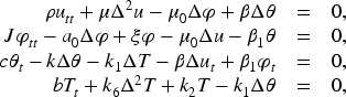
Here the associated system is

\begin{array}{rcl} ρ u_{t t} + μ Δ^{2} u - μ_{0} Δ φ & = & 0, \\ J φ_{t t} - a_{0} Δ φ + ξ φ - μ_{0} Δ u + μ_{2} Δ T - β_{1} θ & = & 0, \\ c θ_{t} - k Δ θ - k_{1} Δ T + β_{1} φ_{t} & = & 0, \\ b T_{t} + k_{6} Δ^{2} T - μ_{2} Δ φ_{t} + k_{2} T - k_{1} Δ θ & = & 0, \end{array}

with the corresponding boundary and initial conditions given by (2) and (3). Now, it is only necessary that

μ_{0} \neq 0.

Otherwise the first uncoupled equation possess stationary solutions. For this system, we can combine the results of the previous case with the results of Section 4 to obtain

i R \subset ϱ (A)

. Here, note that convergence (22) holds, so the arguments are more simple than in the previous case.

On the other hand, for the proof of condition (a) of Theorem 6.1, note that the resolvent equation (28) is

\begin{aligned} i λ u - v = & f_{1} in H^{2} (Ω) \cap H_{0}^{1} (Ω) \\ i λ ρ v + μ Δ^{2} u - μ_{0} Δ φ = & ρ f_{2} in L^{2} (Ω) \\ i λ φ - ψ = & f_{3} in H_{0}^{1} (Ω) \\ i λ J ψ - a_{0} Δ φ + ξ φ - μ_{0} Δ u + μ_{2} Δ T - β_{1} θ = & J f_{4} in L^{2} (Ω) \\ i λ c θ - k Δ θ - k_{1} Δ T + β_{1} ψ = & c f_{5} in L^{2} (Ω) \\ i λ b T + k_{6} Δ^{2} T - μ_{2} Δ ψ + k_{2} T - k_{1} Δ θ = & b f_{6} in L^{2} (Ω) . \end{aligned}

For this resolvent system, note that Lemmas 4.2 and 4.3 hold. Moreover, it is not difficult to see that Lemmas 6.3 and 6.4 are also hold. So, as previously, doing

2 ρ

(74)+(75), we obtain

ρ | | v | |_{L^{2}}^{2} + | | Δ u | |_{L^{2}}^{2} + | | \nabla φ | |_{L^{2}}^{2} \leq C | λ |^{2} | | ψ | |_{L^{2}} | | v | |_{L^{2}} + J | | ψ | |_{L^{2}}^{2} + C | λ | | | U | |_{H} | | F | |_{H} + C | | U | |_{H} | | \nabla θ | |_{L^{2}},

which implies, taking

| λ |

large enough and using Lemma 4.3, that

\begin{array}{rcl} \frac{ρ}{2} | | v | |_{L^{2}}^{2} + | | Δ u | |_{L^{2}}^{2} + | | \nabla φ | |_{L^{2}}^{2} & \leq & C | λ |^{4} | | ψ | |_{L^{2}}^{2} + C | λ | | | U | |_{H} | | F | |_{H} + C | | U | |_{H} | | \nabla θ | |_{L^{2}} \\ \leq & C | λ |^{4} (| | U | |_{H} | | F | |_{H} + | | U | |_{H}^{1 / 2} | | F | |_{H}^{1 / 2} (| | Δ u | |_{L^{2}} + | | \nabla φ | |_{L^{2}})) \\ + C | λ | | | U | |_{H} | | F | |_{H} + C | | U | |_{H} | | \nabla θ | |_{L^{2}}, \end{array}

this is

\frac{ρ}{2} | | v | |_{L^{2}}^{2} + \frac{1}{2} | | Δ u | |_{L^{2}}^{2} + \frac{1}{2} | | \nabla φ | |_{L^{2}}^{2} \leq C | λ |^{8} | | U | |_{H} | | F | |_{H} + C | | U | |_{H} | | \nabla θ | |_{L^{2}} .

Therefore, combining with Lemma 4.2, we conclude that

| | U | |_{L^{2}} \leq C | λ |^{8} | | F | |_{H}, for all | λ | large enough .

Consequently, condition (a) of Theorem 6.1 holds for

r = 8

. This implies polynomial stability of the solutions of the system in the case

β = 0

and

μ_{2} \neq 0

6.3. Case $β \neq 0$ and $μ_{2} = 0$

Here, the system is given by

\begin{array}{rcl} ρ u_{t t} + μ Δ^{2} u - μ_{0} Δ φ + β Δ θ & = & 0, \\ J φ_{t t} - a_{0} Δ φ + ξ φ - μ_{0} Δ u - β_{1} θ & = & 0, \\ c θ_{t} - k Δ θ - k_{1} Δ T - β Δ u_{t} + β_{1} φ_{t} & = & 0, \\ b T_{t} + k_{6} Δ^{2} T + k_{2} T - k_{1} Δ θ & = & 0, \end{array}

with the corresponding boundary and initial conditions given by (2) and (3). In this case, note that

μ_{0}

and

β_{1}

can not be zero simultaneously, this is

| β_{1} | + | μ_{0} | \neq 0.

Otherwise we are leading with an oscillatory solutions. First, as in the previous cases and taking advantage of (25) because

β \neq 0

, we can conclude that

i R \subset ϱ (A)

. For the proof of condition (a) of Theorem 6.1, we analyse the following situations depending on

μ_{0}

and

β_{1}

6.3.1. Sub-Case $μ_{0} β_{1} \neq 0$

In this case Lemmas 4.2, 6.2 and 6.4 are hold. Additionally, in order to estimate $| | v | |_{L^{2}}$ , developing similar arguments used in the proof of Lemma 4.5, but now using Lemma 6.3 instead of Lemma 4.3, we deduce

| | v | |_{L^{2}}^{2} \leq C | | U | |_{H} | | F | |_{H} + C | λ | | | U | |_{H} | | \nabla θ | |_{L^{2}} + C | | F | |^{2} + C | | U | |_{H}^{1 / 2} | | F | |_{H}^{1 / 2} (| | \nabla φ | |_{L^{2}} + | | Δ u | |_{L^{2}}) .

So, multiplying the previous estimative by

2 ρ

, the estimative given in 6.2 by

2 J

and adding to estimative given in Lemma 6.4, we obtain

\begin{array}{rcl} ρ | | v | |_{L^{2}}^{2} + J | | ψ | |_{L^{2}}^{2} + | | Δ u | |_{L^{2}}^{2} + | | \nabla φ | |_{L^{2}}^{2} & \leq & C | | U | |_{H} | | F | |_{H} + C | | U | |_{H}^{1 / 2} | | F | |_{H}^{1 / 2} (| | Δ u | |_{L^{2}} + | | \nabla φ | |_{L^{2}}) \\ + C | λ | | | U | |_{H} | | \nabla θ | |_{L^{2}} + C | | F | |_{H}^{2}, \end{array}

this is

ρ | | v | |_{L^{2}}^{2} + J | | ψ | |_{L^{2}}^{2} + \frac{1}{2} | | Δ u | |_{L^{2}}^{2} + \frac{1}{2} | | \nabla φ | |_{L^{2}}^{2} \leq C | | U | |_{H} | | F | |_{H} + C | λ | | | U | |_{H} | | \nabla θ | |_{L^{2}} + C | | F | |_{H}^{2} .

So, combining with Lemma 4.2, we conclude

| | U | |_{H}^{2} \leq C | λ |^{2} | | U | |_{H} | | F | |_{H} + C | | F | |_{H}^{2} ⟹ | | U | |_{H} \leq C | λ |^{2} | | F | |_{H},

for all

| λ |

large enough. Then, condition (a) of Theorem 6.1 holds for

r = 2

, which implies polynomial stability.

6.3.2. Sub-Case $μ_{0} = 0$ and $β_{1} \neq 0$

In this case, the results are analogous to the previous sub-case, with $r = 2$ .

6.3.3. Sub-Case $μ_{0} \neq 0$ and $β_{1} = 0$

In this case, the resolvent system (28) is given by

\begin{array}{rcl} i λ u - v & = & f_{1} in H^{2} (Ω) \cap H_{0}^{1} (Ω) \\ i λ ρ v + μ Δ^{2} u - μ_{0} Δ φ + β Δ θ & = & ρ f_{2} in L^{2} (Ω) \\ i λ φ - ψ & = & f_{3} in H_{0}^{1} (Ω) \\ i λ J ψ - a_{0} Δ φ + ξ φ - μ_{0} Δ u & = & J f_{4} in L^{2} (Ω) \\ i λ c θ - k Δ θ - k_{1} Δ T - β Δ v & = & c f_{5} in L^{2} (Ω) \\ i λ b T + k_{6} Δ^{2} T + k_{2} T - k_{1} Δ θ & = & b f_{6} in L^{2} (Ω) . \end{array}

(76)

For this resolvent system, note that Lemma 4.2 holds. Taking into account that

β_{1} = 0

, the estimative given by Lemma 4.5 is also true. This is

| | v | |_{L^{2}}^{2} \leq C | | U | |_{H} | | F | |_{H} + C | | U | |_{H}^{1 / 2} | | F | |_{H}^{1 / 2} (| | Δ u | |_{L^{2}} + | | \nabla φ | |_{L^{2}})

(77)

Moreover, multiplying (76)

_{5}

v

L^{2}

, using Lemma 4.2, we can deduce

| | \nabla v | |_{L^{2}}^{2} \leq C | λ |^{2} | | U | |_{H} | | F | |_{H},

(78)

for all

| λ |

large enough. On the other hand, multiplying (76)

_{2}

u

L^{2}

results

μ | | Δ u | |_{L^{2}}^{2} = ρ | | v | |_{L^{2}}^{2} + ρ (f_{1}, v)_{L^{2}} - \underset{J_{3}}{\underset{⏟}{μ_{0} (\nabla φ, \nabla u)_{L^{2}}}} - β (θ, Δ u)_{L^{2}} + ρ (f_{2}, u)_{L^{2}}

where, taking into account (76)

_{1}

we obtain

| J_{3} | = | μ_{0} {(\nabla φ, \frac{\nabla v + \nabla f_{1}}{i λ})}_{L^{2}} | \leq C | | U | |_{H} | | F | |_{H} + C | | \nabla φ | |_{L^{2}} (\frac{| | \nabla v | |_{L^{2}}}{| λ |}),

for all

| λ |

large enough. So, from the previous equality and using (77) and (78), we deduce that

| | Δ u | |_{L^{2}}^{2} \leq C | | U | |_{H} | | F | |_{H} + C | | U | |_{H}^{1 / 2} | | F | |_{H}^{1 / 2} (| | Δ u | |_{L^{2}} + | | \nabla φ | |_{L^{2}}),

which implies

| | Δ u | |_{L^{2}}^{2} \leq C | | U | |_{H} | | F | |_{H} + C | | U | |_{H}^{1 / 2} | | F | |_{H}^{1 / 2} | | \nabla φ | |_{L^{2}} .

(79)

Analogously, multiplying (76)

_{2}

φ \in L^{2}

results

μ_{0} | | \nabla φ | |_{L^{2}}^{2} = - i λ ρ (v, φ)_{L^{2}} - \underset{J_{4}}{\underset{⏟}{μ (Δ u, Δ φ)_{L^{2}}}} + β (\nabla θ, \nabla φ)_{L^{2}} + ρ (f_{2}, φ)_{L^{2}} .

Here, using (76)

_{4}

we deduce

J_{4} = - \frac{i λ μ_{0} J}{a_{0}} (Δ u, ψ,)_{L^{2}} - \frac{μ_{0} ξ}{a_{0}} (\nabla u, \nabla φ)_{L^{2}} - \frac{μ μ_{0}}{a_{0}} | | Δ u | |_{L^{2}}^{2} - \frac{μ J}{a_{0}} (Δ u, f_{2})_{L^{2}} .

So, from the same arguments used to estimate

J_{3}

, we obtain

| J_{4} | \leq C | | U | |_{H} | | F | |_{H} + C | λ | | | ψ | |_{L^{2}} | | Δ u | |_{L^{2}} + C | | Δ u | |_{L^{2}}^{2} + C | | \nabla φ | |_{L^{2}} (\frac{| | \nabla v | |_{L^{2}}}{| λ |}),

Therefore, substituting this estimative in the previous equality, using (78) and Lemma 4.2 we deduce

| | \nabla φ | |_{L^{2}}^{2} \leq C | | U | |_{H} | | F | |_{H} + C | λ |^{2} | | v | |_{L^{2}}^{2} + C | λ | | | ψ | |_{L^{2}} | | Δ u | |_{L^{2}} + C | | Δ u | |_{L^{2}}^{2},

which implies, using (77) and (79),

| | \nabla φ | |_{L^{2}}^{2} \leq C | λ |^{4} | | U | |_{H} | | F | |_{H} + C | λ | | | ψ | |_{L^{2}} | | Δ u | |_{L^{2}},

(80)

for all

| λ |

large enough. Additionally, multiplying (76)

_{3}

ψ \in L^{2}

we deduce

| | ψ | |_{L^{2}}^{2} \leq C | λ |^{2} | | \nabla φ | |_{L^{2}}^{2} | + C | | U | |_{H} | | F | |_{H},

which, after (80), brings to

| | ψ | |_{L^{2}}^{2} \leq C | λ |^{6} | | U | |_{H} | | F | |_{H} + C | λ |^{6} | | Δ u | |_{L^{2}}^{2},

(81)

for all

| λ |

large enough. Therefore, adding (80) and (81) we obtain

| | \nabla φ | |_{L^{2}}^{2} + | | ψ | |_{L^{2}}^{2} \leq C | λ |^{6} | | U | |_{H} | | F | |_{H} + C | λ |^{6} | | Δ u | |_{L^{2}}^{2} .

So, combining with (79) we get

| | Δ u | |_{L^{2}}^{2} + \frac{1}{2} | | \nabla φ | |_{L^{2}}^{2} + | | ψ | |_{L^{2}}^{2} \leq C | λ |^{12} | | U | |_{H} | | F | |_{H},

for all

| λ |

large enough. Finally, combining with Lemma 4.2 and (77), it is not difficult to see

| | U | |_{H} \leq C | λ |^{12} | | F | |_{H},

for all

| λ |

large enough. Then, condition (a) of Theorem 6.1 holds for

r = 12

, which implies polynomial stability.

In summary, in this section we have proved the following theorem.

Theorem 6.5

Let us assume condition (4) on the constants of the system. Assuming, additionally, that $μ_{2} β = 0$ , then the associated semigroup to the thermoelastic plate problems (1)–(3) is polynomially stable where the corresponding rates of decay are associated to the following cases (1)

If $β = 0$ and $μ_{2} = 0$ , then

| | e^{t A} A^{- 1} | |_{L (H)} \leq O (t^{- 1 / 10}), \forall t \geq t_{0} .

(2)

If $β = 0$ and $μ_{2} \neq 0$ , then

| | e^{t A} A^{- 1} | |_{L (H)} \leq O (t^{- 1 / 8}), \forall t \geq t_{0} .

(3)

If $β \neq 0$ , $μ_{2} = 0$ and $| β_{1} | + | μ_{0} | \neq 0$ , then

| | e^{t A} A^{- 1} | |_{L (H)} \leq O (t^{- 1 / 2}), \forall t \geq t_{0} .

Remark 6.6

The previous theorem shows polynomial rates of decay, which probably are not optimal. The optimality of the polynomial rates of decay remains as a open question.

Footnotes

Funding

The author(s) disclosed receipt of the following financial support for the research, authorship, and/or publication of this article: Hugo D Fernández Sare is supported by Conselho Nacional de Desenvolvimento Científico e Tecnológico CNPq — Brazil grant 406621/2021-7 and Fundação de Amparo à Pesquisa do Estado de Minas Gerais FAPEMIG — Brazil grant APQ-00782-21.

Declaration of Conflicting Interests

The authors declared no potential conflicts of interest with respect to the research, authorship, and/or publication of this article.

Orcid iDs

Hugo D Fernández Sare

Ramón Quintanilla

References

Borichev

Tomilov

(2010). Optimal polynomial decay of functions and operator semigroup. Mathematische Annalen, 347, 455–478.

Casas

Quintanilla

(2005). Exponential stability in thermoelasticity with microtemperatures. International Journal of Engineering Science, 43(1–2), 33–47.

Cowin

S. C.

(1985). The viscoelastic behavior of linear elastic materials with voids. Journal of Elasticity, 15, 185–191.

Cowin

S. C.

Nunziato

J. W.

(1983). Linear elastic materials with voids. Journal of Elasticity, 13, 125–147.

Dafermos

C. M.

(1976). Contraction semigroups and trend to equilibrium in continuum mechanics. Lecture Notes in Mathematics, 503, 295–306.

Engel

K.-J.

Nagel

(2000). One-parameter semigroups for linear evolution equations. Springer-Verlag.

Fernández Sare

H. D.

Quintanilla

(2021). Porous-elastic plates: Fourier versus type III. Applied Mathematics and Optimization, 84, 1055–1085.

Green

A. E.

Lindsay

K. A.

(1972). Thermoelasticity. Journal of Elasticity, 2, 1–7.

Huang

F. L.

(1985). Characteristic conditions for exponential stability of linear dynamical systems in Hilbert spaces. Annals of Differential Equations, 1(1), 43–56.

10.

Ieşan

(2007). Thermoelasticity of bodies with microstructure and microtemperatures. International Journal of Solids and Structures, 44, 8648–8662.

11.

Ieşan

Quintanilla

(2000). On a theory of thermoelastic with microtemperatures. Journal of Thermal Stresses, 20(3), 199–215.

12.

Liu

Quintanilla

(2010). Analyticity of solutions in type III thermoelastic plates. IMA Journal of Applied Mathematics, 75, 356–365.

13.

Liu

Quintanilla

Wang

(2022). On the regularity and stability of three-phase-lag thermoelastic plates. Applicable Analysis, 101, 5376–5385.

14.

Liu

Renardy

(1995). A note on the equations of a thermoelastic plates. Applied Mathematics Letters, 8, 1–6.

15.

Liu

Zheng

(1999). Semigroups associated with dissipative systems (Vol. 398, Research notes in mathematics).. Chapman & Hall/CRC Press.

16.

Pazy

(1983). Semigroups of linear operators and applications to partial differential equations. Springer-Verlag.

17.

Prüss

(1984). On the spectrum of

C_{0}

-semigroups. Transactions of the American Mathematical Society, 284(2), 847–857.

18.

Quintanilla

Racke

(2011). Addendum to: Qualitative aspects of solutions in resonators. Archives of Mechanics, 63(4), 429–435.

19.

Quintanilla

Racke

Ueda

(2023). Decay for thermoelastic Green–Lindsay plates in bounded and unbounded domains. Communications on Pure and Applied Analysis, 22, 167–191.

Stability of Thermoelastic Plates With Voids and Micro-Temperatures

Abstract

Keywords

1. Introduction

2. Model

5.1. Lack of Exponential Stability

6.3. Case β ≠ 0 and μ 2 = 0

6.3.1. Sub-Case μ 0 β 1 ≠ 0

6.3.2. Sub-Case μ 0 = 0 and β 1 ≠ 0

6.3.3. Sub-Case μ 0 ≠ 0 and β 1 = 0

Footnotes

Funding

Declaration of Conflicting Interests

Orcid iDs

References

6.3. Case $β \neq 0$ and $μ_{2} = 0$

6.3.1. Sub-Case $μ_{0} β_{1} \neq 0$

6.3.2. Sub-Case $μ_{0} = 0$ and $β_{1} \neq 0$

6.3.3. Sub-Case $μ_{0} \neq 0$ and $β_{1} = 0$