Well-Posedness and Long-Time Dynamics of a Water-Waves Model With Time-Varying Boundary Delay

Abstract

A higher-order nonlinear Boussinesq system with a time-dependent boundary delay is considered. Sufficient conditions are presented to ensure the well-posedness of the problem by utilizing Kato’s variable norm technique and the Fixed Point Theorem. More significantly, the energy decay for the linearized problem is demonstrated using the energy method.

Keywords

higher-order Boussinesq system stabilization delay decay rate Lyapunov approach

1. Introduction

1.1. Background

The Boussinesq system comprises a set of nonlinear partial differential equations that model wave dynamics in fluids with small amplitude and long wavelengths. Originally formulated by the French mathematician Joseph Boussinesq in the 19th century to describe shallow water waves (Boussinesq, 1871), since then, the system has been recognized as a model for various physical phenomena, including ocean currents, atmospheric circulation, and heat transfer in fluids. Consequently, the Boussinesq system remains an essential tool in numerous fluid dynamics, with broad applications in fields such as meteorology, oceanography, and engineering.

In more recent studies, Bona et al. (2002, 2004) introduced a four-parameter family of Boussinesq systems to describe the motion of small-amplitude long waves on the surface of an ideal fluid under gravity, particularly in scenarios where the motion is predominantly two-dimensional. In particular, Bona et al. (2002, 2004) investigated the following system:

\begin{aligned} {\begin{cases} η_{t} + ω_{x} + a ω_{x x x} - b η_{t x x} + a_{1} ω_{x x x x x} + b_{1} η_{t x x x x} \\ = - (η ω)_{x} + b (η ω)_{x x x} - α^{'} (η ω_{x x})_{x}, \\ ω_{t} + η_{x} + c η_{x x x} - d ω_{t x x} + c_{1} η_{x x x x x} + d_{1} ω_{t x x x x} \\ = - ω ω_{x} - c (ω ω_{x})_{x x} - (η η_{x x})_{x} + β^{'} ω_{x} ω_{x x} + ρ ω ω_{x x x} . \end{cases} \end{aligned}

(1.1)

In this context, $η$ represents the elevation of the fluid surface from its equilibrium position, while $ω = ω_{θ}$ denotes the horizontal velocity of the flow at a height $θ h$ , where $h$ is the undisturbed depth of the fluid and $θ$ is a constant within the interval $[0, 1]$ . The variables $x$ and $t$ correspond to space and time, respectively, and the physical parameters $a, b, c, d, a_{1}, c_{1}, b_{1}, d_{1}$ must satisfy the following relationships:

\begin{aligned} {\begin{cases} \begin{array}{ll} a + b = \frac{1}{2} (θ^{2} - \frac{1}{3}), c + d = \frac{1}{2} (1 - θ^{2}), \\ a_{1} - b_{1} = - \frac{1}{2} (θ^{2} - \frac{1}{3}) b + \frac{5}{24} {(θ^{2} - \frac{1}{5})}^{2}, \\ c_{1} - d_{1} = \frac{1}{2} (1 - θ^{2}) c + \frac{5}{24} (1 - θ^{2}) (θ^{2} - \frac{1}{5}), \\ α^{'} = a + b - \frac{1}{3}, β^{'} = c + d - 1, ρ = c + d . \end{array} \end{cases} \end{aligned}

Stabilization results for the higher-order system (1.1) on the periodic domain were established in Bautista and Pazoto (2020b) under the conditions $a_{1} = c_{1} = 0$ , with general damping applied to each equation. Furthermore, the local exact controllability of system (1.1) was investigated in Bautista et al. (2021), where the control is localized within the interior of the domain and influences only one equation.

Negative controllability results are explored in Bautista and Pazoto (2020a) and Sierra Fonseca and Pazoto (2022) when the third- and fifth-order Korteweg–de Vries (KdV) terms are removed from the system mentioned above, that is, (1.1) with $a = a_{1} = c = c_{1} = 0$ . In this case, the system consists of two coupled Benjamin–Bona–Mahony-type equations. The authors demonstrated that the linear model is approximately controllable but not spectrally controllable. This implies that although any state can be brought arbitrarily close to another, no finite linear combination of eigenfunctions, other than zero, can be driven to zero.

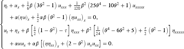
Let us now consider $b = d = b_{1} = d_{1} = 0$ and make a scaling argument to obtain the fifth-order Boussinesq system

{\begin{cases} η_{t} + ω_{x} + a ω_{x x x} + a_{1} ω_{x x x x x} = - (η ω)_{x} - α^{'} (η ω_{x x})_{x}, \\ ω_{t} + η_{x} + c η_{x x x} + c_{1} η_{x x x x x} = - ω ω_{x} - c (ω ω_{x})_{x x} - (η η_{x x})_{x} + β^{'} ω_{x} ω_{x x} + ρ ω ω_{x x x} . \end{cases}

(1.2)

In the above system, we note that

c, a_{1} \geq 0

. Thus, we consider the following case:

a = c > 0, and c_{1} = a_{1} > 0.

(1.3)

It is important to highlight that, to the best of our knowledge, there are no existing results that combine a damping mechanism with a boundary time-varying delay to achieve stabilization of the higher-order Boussinesq system associated with (1.2). This gap forms the main motivation for the present work. It is also worth emphasizing the practical prevalence of time delays in control systems, a phenomenon that is virtually unavoidable due to factors such as the lag between sensors, actuators, and data processing. In light of this, significant efforts have been made to mitigate or eliminate the effects of constant time delays. For example, stability results under smallness conditions on the domain length $L$ and the initial data have been established in Baudouin et al. (2019) and Valein (2022) for the KdV equation and in Capistrano-Filho et al. (2023) for the Kawahara equation. In the case of time-dependent delays, similar results have been obtained in Parada et al. (2023) for the KdV equation and Capistrano-Filho et al. (2024) for the coupled KdV–KdV system.

1.2. Notations and Main Results

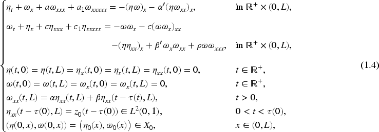
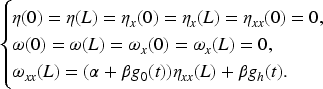
This article is concerned with the following system:

{\begin{cases} η_{t} + ω_{x} + a ω_{x x x} + a_{1} ω_{x x x x x} = - (η ω)_{x} - α^{'} (η ω_{x x})_{x}, & in R^{+} \times (0, L), \\ ω_{t} + η_{x} + c η_{x x x} + c_{1} η_{x x x x x} = - ω ω_{x} - c (ω ω_{x})_{x x} \\ - (η η_{x x})_{x} + β^{'} ω_{x} ω_{x x} + ρ ω ω_{x x x}, & in R^{+} \times (0, L), \\ η (t, 0) = η (t, L) = η_{x} (t, 0) = η_{x} (t, L) = η_{x x} (t, 0) = 0, & t \in R^{+}, \\ ω (t, 0) = ω (t, L) = ω_{x} (t, 0) = ω_{x} (t, L) = 0, & t \in R^{+}, \\ ω_{x x} (t, L) = α η_{x x} (t, L) + β η_{x x} (t - τ (t), L), & t > 0, \\ η_{x x} (t - τ (0), L) = z_{0} (t - τ (0)) \in L^{2} (0, 1), & 0 < t < τ (0), \\ (η (0, x), ω (0, x)) = (η_{0} (x), ω_{0} (x)) \in X_{0}, & x \in (0, L), \end{cases}

(1.4)

where the parameters

a, c, a_{1}, c_{1}

verify (1.3). Moreover, we assume that there exist positive constants

τ_{0}

M

, and

d < 1

such that the time-dependent delay function

τ (t)

satisfies the following standard conditions:

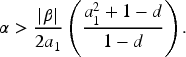
{\begin{cases} 0 < τ_{0} \leq τ (t) \leq M, \dot{τ} (t) \leq d < 1, & \forall t \geq 0, \\ τ \in W^{2, \infty} ([0, T]), & T > 0. \end{cases}

(1.5)

Finally, the feedback gains $α > 0$ and $β$ must obey the following constraint:

The matrix Φ_{α, β} = (\begin{matrix} - 2 a_{1} α + | β | & - a_{1} β \\ - a_{1} β & | β | (d - 1) \end{matrix}) is negative definite .

(1.6)

The condition (1.6) ensures the dissipation of system (1.4). It is worth mentioning that a similar condition is used for other types of delayed dispersive systems (see, for instance, Capistrano-Filho et al., 2024; Parada et al., 2023). Furthermore, recalling that

0 \leq d < 1

and

a_{1} > 0

, one can readily check that (1.6) is fulfilled if, for instance, the feedback gains

α

and

β

satisfy

α > \frac{| β |}{2 a_{1}} (\frac{a_{1}^{2} + 1 - d}{1 - d}) .

Next, let $X_{0} := L^{2} (0, L) \times L^{2} (0, L),$ and the state space

H := X_{0} \times L^{2} (0, 1)

equipped with the inner product

\begin{aligned} {⟨ (η, ω, z), (\tilde{η}, \tilde{ω}, \tilde{z}) ⟩}_{t} = & {⟨ (η, ω), (\tilde{η}, \tilde{ω}) ⟩}_{X_{0}} + | β | τ (t) {⟨ z, \tilde{z} ⟩}_{L^{2} (0, 1)}, \end{aligned}

for any

(η, ω; z), (\tilde{η}, \tilde{ω}; \tilde{z}) \in H

. Moreover, we shall consider the space

B := C ([0, T], X_{0}) \cap L^{2} (0, T, [H_{0}^{2} (0, L)]^{2}),

whose norm is

‖ (η, ω) ‖_{B} = sup_{t \in [0, T]} ‖ (η (t), ω (t)) ‖_{X_{0}} + ‖ (η, ω) ‖_{L^{2} (0, T, [H_{0}^{2} (0, L)]^{2})} .

To present our first result, let us introduce the following space:

X_{3} := {(η, ω) \in {[H^{3} (0, L) \cap H_{0}^{2} (0, L)]}^{2} | η_{x x} (0) = 0} .

(1.7)

The first result of this manuscript ensures the local well-posedness of system (1.4).

Theorem 1.1

Let $T > 0$ and suppose the parameters $a, c, a_{1}, c_{1}$ verify (1.3). Then, there exists $θ = θ (T) > 0$ such that, for every $(η_{0}, ω_{0}; z_{0}) \in X_{3} \times L^{2} (0, 1)$ satisfying

{‖ (η_{0}, ω_{0}) ‖}_{[H^{3} (0, L) \cap H_{0}^{2} (0, L)]^{2}} < θ,

the system (1.4) admits a unique solution

(η, ω) \in C ([0, T]; X_{3})

. Moreover

‖ (η, ω) ‖_{C ([0, T] : [H^{3} (0, L) \cap H_{0}^{2} (0, L)]^{2})} \leq C {‖ (η_{0}, u_{0}) ‖}_{[H^{3} (0, L) \cap H_{0}^{2} (0, L)]^{2}},

for some positive constant,

C = C (T)

Our second result is closely related to the total energy associated with system (1.4) that is defined in $H$ by

E (t) = \frac{1}{2} \int_{0}^{L} (η^{2} (t, x) + ω^{2} (t, x)) d x + \frac{| β |}{2} τ (t) \int_{0}^{1} η_{x x}^{2} (t - τ (t) ρ, L) d ρ .

(1.8)

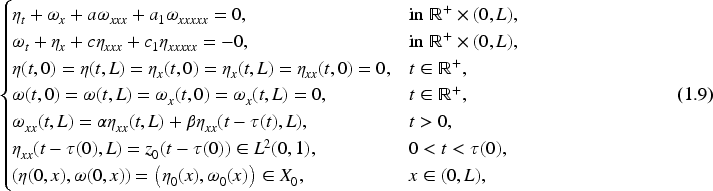
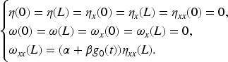
Indeed, the second result of the article guarantees that the energy

E (t)

associated with the following system:

{\begin{cases} η_{t} + ω_{x} + a ω_{x x x} + a_{1} ω_{x x x x x} = 0, & in R^{+} \times (0, L), \\ ω_{t} + η_{x} + c η_{x x x} + c_{1} η_{x x x x x} = - 0, & in R^{+} \times (0, L), \\ η (t, 0) = η (t, L) = η_{x} (t, 0) = η_{x} (t, L) = η_{x x} (t, 0) = 0, & t \in R^{+}, \\ ω (t, 0) = ω (t, L) = ω_{x} (t, 0) = ω_{x} (t, L) = 0, & t \in R^{+}, \\ ω_{x x} (t, L) = α η_{x x} (t, L) + β η_{x x} (t - τ (t), L), & t > 0, \\ η_{x x} (t - τ (0), L) = z_{0} (t - τ (0)) \in L^{2} (0, 1), & 0 < t < τ (0), \\ (η (0, x), ω (0, x)) = (η_{0} (x), ω_{0} (x)) \in X_{0}, & x \in (0, L), \end{cases}

(1.9)

decays exponentially, even in the presence of delay, and provides an estimate of the decay rate. The result is expressed as follows:

Theorem 1.2

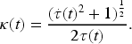
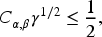
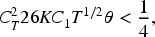
Let the parameters $a, c, a_{1}, c_{1}$ verify (1.3) and $0 < L < \sqrt{(5 a_{1} / 3 a)} π$ . Suppose also that the time-dependent delay function satisfies (1.5). Then, there exist two positive constants

ζ = \frac{1 + max {μ_{1} L, μ_{2}}}{1 - max {μ_{1} L, μ_{2}}},

(1.10)

and

\begin{aligned} λ \leq min {\frac{μ_{1} π^{2} (5 a_{1} π^{2} - 3 a L^{2})}{L^{4} (1 + μ_{1} L)}, \frac{μ_{2} (1 - d)}{M (1 + μ_{2})}}, \end{aligned}

(1.11)

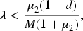
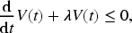
such that the energy

E (t)

given by (1.8) associated with system (1.9) satisfies

E (t) \leq ζ E (0) e^{- λ t}, for all t \geq 0.

Here

μ_{1}

and

μ_{2}

are two positive constants small enough to be well-chosen.

The main contribution of this work is to establish the local well-posedness of system (1.2) and prove the exponential stability of system (1.9). These results extend and refine those obtained in Capistrano-Filho et al. (2024) and Parada et al. (2023) in several significant directions. More specifically, unlike Capistrano-Filho et al. (2024), where the nonlinear coupling appears only in one equation through the term $(η ω)_{x}$ , our model introduces an additional nonlinear coupling term of the form $(η ω_{x x})_{x}$ . Furthermore, while Capistrano-Filho et al. (2024) feature a single uncoupled nonlinear term, our system includes four additional uncoupled nonlinear terms of higher order, making the analysis more intricate and requiring careful handling of the extra terms in the computations. In particular, in our case, the higher-order spatial derivatives (of order three and five) appear with positive signs, leading to conflicts between the $H^{1}$ and $H^{2}$ -norm terms during integration by parts. Compared to Parada et al. (2023), the situation is even more complex: the problem in Parada et al. (2023) involves a single uncoupled equation with only one nonlinearity and a highest-order derivative of three. Finally, and importantly, in contrast to Capistrano-Filho et al. (2024) and Parada et al. (2023), we employ the transposition method (Capistrano-Filho et al., 2019) to address the well-posedness of our system.

1.3. Outline

The structure of the paper is as follows. In Section 2, we establish the well-posedness of the nonlinear problem (1.4), namely, we show Theorem 1.1 starting with an analysis of the linear system (1.9) using the variable norm technique of Kato, followed by the application of the Fixed Point Theorem to prove well-posedness of the full nonlinear problem. Section 3 focuses on the stability result presented in Theorem 1.2, along with a discussion of the optimal decay rate. Finally, we conclude the paper with further remarks in Section 4.

2. Well-Posedness Results

In the sequel, we will assume $a = c > 0$ and $a_{1} = c_{1} > 0$ in (1.4) as well as in (1.9). We will first examine the well-posedness of the linear system (1.9) and subsequently analyze the properties of the nonlinear problem (1.4) in suitable spaces.

2.1. Linear Problem

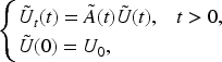
Consider the following linear Cauchy problem:

{\begin{cases} \frac{d}{d t} U (t) = A (t) U (t), & t > 0, \\ U (0) = U_{0}, & t > 0, \end{cases}

(2.1)

where

A (t) : D (A (t)) \subset H \to H

is densely defined, and

D (A (t))

is independent of time

t

, that is,

D (A (t)) = D (A (0)),

for all

t > 0.

The next theorem ensures the existence and uniqueness of the Cauchy problem (2.1).

Theorem 2.1 (Kato, 1970)

Assume that:

(1)
$Z = D (A (0))$ is a dense subset of $H$ and $D (A (t)) = D (A (0))$ , for all $t > 0$ .
(2)
$A (t)$ generates a strongly continuous semigroup on $H$ . Moreover, the family ${A (t) : t \in [0, T]}$ is stable with stability constants $C a n d m$ independent of $t$ .
(3)
$\partial_{t} A (t)$ belongs to $L_{}^{\infty} ([0, T], B (Z, H))$ , the space of equivalent classes of essentially bounded, strongly measurable functions from $[0, T]$ into the set $B (Z, H)$ of bounded operators from $Z$ into $H$ .
Then, problem (2.1) has a unique solution $U \in C ([0, T], Z) \cap C^{1} ([0, T], H)$ for any initial datum in $Z$ .

The task ahead is to apply the above result to ensure the existence of solutions for the linear system (1.9). Arguing as in Xu et al. (2006), Nicaise and Pignotti (2006), and Nicaise et al. (2009), let us define the auxiliary variable
$z (t, ρ) = η_{x x} (t - τ (t) ρ, L),$
which satisfies the transport equation:
${\begin{cases} τ (t) z_{t} (t, ρ) + (1 - \dot{τ} (t) ρ) z_{ρ} (t, ρ) = 0, & t > 0, ρ \in (0, 1), \\ z (t, 0) = η_{x x} (t, L), z (0, ρ) = z_{0} (- τ (0) ρ), & t > 0, ρ \in (0, 1) . \end{cases}$
(2.2)

Now, we pick up $U = (η, ω; z)^{T}$ and consider the time-dependent operator
$A (t) : D (A (t)) \subset H \to H,$
given by
$A (t) (η, ω, z) := (- ω_{x} - a ω_{x x x} - a_{1} ω_{x x x x x}, - η_{x} - a η_{x x x} - a_{1} η_{x x x x x}, \frac{\dot{τ} (t) ρ - 1}{τ (t)} z_{ρ}),$
(2.3)
with a domain defined by
$D (A (t)) = {\begin{aligned} (η, ω, z) \in H; & (η, ω) \in {[H^{5} (0, L) \cap H_{0}^{2} (0, L)]}^{2}, z \in H^{1} (0, 1), \\ η_{x x} (0) = 0, z (0) = η_{x x} (L), ω_{x x} (L) = α η_{x x} (L) + β z (1) \end{aligned}} .$
(2.4)
This allows us to write problem (1.9) in the abstract form (2.1) by using (2.2)–(2.4). Additionally, it is noteworthy that $D (A (t))$ is independent of time $t$ since $D (A (t)) = D (A (0))$ .

Now, taking the triplet ${A, H, Z}$ , with $A = {A (t) : t \in [0, T]}$ , for some $T > 0$ fixed and $Z = D (A (0))$ , we can state and prove the well-posedness result of (2.1) related to ${A, H, Z}$ .
Theorem 2.2
Let the parameters $a, c, a_{1}, c_{1}$ verify (1.3). Assume that $α$ and $β$ are real constants such that (1.6) holds. Taking $U_{0} \in H$ , there exists a unique solution $U \in C ([0, + \infty), H)$ to (2.1) whose operator is defined by (2.3)–(2.4). Moreover, if $U_{0} \in D (A (0))$ , then $U \in C ([0, + \infty), D (A (0))) \cap C^{1} ([0, + \infty), H) .$
Proof.
The result will be proved in a standard way (see, for instance, Nicaise et al., 2009). First, it is not difficult to see that $Z = D (A (0))$ is a dense subset of $H$ and $D (A (t)) = D (A (0))$ , for all $t > 0$ . Thus, the requirement (1) of Theorem 2.1 is fulfilled.

Concerning the condition (2) of Theorem 2.1, let us note that simple integrations by parts together with the boundary conditions yield
${⟨ A (t) U, U ⟩}_{t} - κ (t) {⟨ U, U ⟩}_{t} \leq \frac{1}{2} (η_{x x} (t, L), η_{x x} (t - τ (t), L)) Φ_{α, β} {(η_{x x} (t, L), η_{x x} (t - τ (t), L))}^{T},$
where
$κ (t) = \frac{(\dot{τ} {(t)}^{2} + 1)^{\frac{1}{2}}}{2 τ (t)} .$
Owing to (1.6), it follows that
${⟨ A (t) U, U ⟩}_{t} - κ (t) {⟨ U, U ⟩}_{t} \leq 0.$
Consequently, $\tilde{A} (t) = A (t) - κ (t) I$ is dissipative.

Now, we claim the following: Claim 1
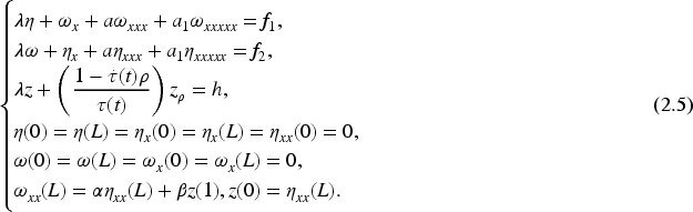
For all $t \in [0, T]$ , the operator $A (t)$ is maximal, or equivalently, we have that $λ I - A (t)$ is surjective, for some $λ > 0$ .
In fact, let us fix $t \in [0, T]$ . Given $(f_{1}, f_{2}, h)^{T} \in H$ , we seek a solution $U = (η, ω, z)^{T} \in D (A (t))$ of the equation $(λ I - A (t)) U = (f_{1}, f_{2}, h)$ , that is,
${\begin{cases} λ η + ω_{x} + a ω_{x x x} + a_{1} ω_{x x x x x} = f_{1}, \\ λ ω + η_{x} + a η_{x x x} + a_{1} η_{x x x x x} = f_{2}, \\ λ z + (\frac{1 - \dot{τ} (t) ρ}{τ (t)}) z_{ρ} = h, \\ η (0) = η (L) = η_{x} (0) = η_{x} (L) = η_{x x} (0) = 0, \\ ω (0) = ω (L) = ω_{x} (0) = ω_{x} (L) = 0, \\ ω_{x x} (L) = α η_{x x} (L) + β z (1), z (0) = η_{x x} (L) . \end{cases}$
(2.5)
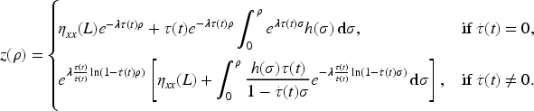
One can readily verify that $z$ is given by
$z (ρ) = {\begin{cases} η_{x x} (L) e^{- λ τ (t) ρ} + τ (t) e^{- λ τ (t) ρ} \int_{0}^{ρ} e^{λ τ (t) σ} h (σ) d σ, & if \dot{τ} (t) = 0, \\ e^{λ \frac{τ (t)}{\dot{τ} (t)} \ln (1 - \dot{τ} (t) ρ)} [η_{x x} (L) + \int_{0}^{ρ} \frac{h (σ) τ (t)}{1 - \dot{τ} (t) σ} e^{- λ \frac{τ (t)}{\dot{τ} (t)} \ln (1 - \dot{τ} (t) σ)} d σ], & if \dot{τ} (t) \neq 0. \end{cases}$
Thereby, $z (1) = η_{x x} (L) g_{0} (t) + g_{h} (t)$ , in which
$g_{0} (t) = {\begin{cases} e^{- λ τ (t)}, & if \dot{τ} (t) = 0, \\ e^{λ \frac{τ (t)}{\dot{τ} (t)} \ln (1 - \dot{τ} (t))}, & if \dot{τ} (t) \neq 0, \end{cases}$
and
$g_{h} (t) = {\begin{cases} τ (t) e^{- λ τ (t)} \int_{0}^{1} e^{λ τ (t) σ} h (σ) d σ, & if \dot{τ} (t) = 0, \\ e^{λ \frac{τ (t)}{\dot{τ} (t)} \ln (1 - \dot{τ} (t))} \int_{0}^{1} \frac{h (σ) τ (t)}{1 - \dot{τ} (t) σ} e^{- λ \frac{τ (t)}{\dot{τ} (t)} \ln (1 - \dot{τ} (t) σ)} d σ, & if \dot{τ} (t) \neq 0. \end{cases}$
Combining the latter with (2.5), it follows that $η$ and $ω$ are solutions of the system
${\begin{cases} λ η + ω_{x} + a ω_{x x x} + a_{1} ω_{x x x x x} = f_{1}, \\ λ ω + η_{x} + a η_{x x x} + a_{1} η_{x x x x x} = f_{2}, \end{cases}$
(2.6)
and satisfy the boundary conditions
${\begin{cases} η (0) = η (L) = η_{x} (0) = η_{x} (L) = η_{x x} (0) = 0, \\ ω (0) = ω (L) = ω_{x} (0) = ω_{x} (L) = 0, \\ ω_{x x} (L) = (α + β g_{0} (t)) η_{x x} (L) + β g_{h} (t) . \end{cases}$
Now, let $ϕ_{1} \in C^{\infty} ([0, L])$ be a function such that $ϕ_{1} (0) = ϕ_{1} (L) = ϕ_{1, x} (0) = ϕ_{1, x} (L) = 0$ and $ϕ_{1, x x} (L) = 1$ . Next, we define a function $ψ (x, \cdot) = ϕ_{1} (x) β g_{h} (\cdot) \in C^{\infty} ([0, L])$ and let $\hat{ω} := ω - ψ$ . This, together with (2.6), implies that $η$ and $ω$ satisfy
${\begin{cases} λ η + ω_{x} + a ω_{x x x} + a_{1} ω_{x x x x x} = f_{1} - (ψ_{x} + ψ_{x x x} + ψ_{x x x x x}) =: \tilde{f_{1}}, \\ λ ω + η_{x} + a η_{x x x} + a_{1} η_{x x x x x} = f_{2} - λ ψ =: \tilde{f_{2}}, \end{cases}$
as well as the boundary conditions
${\begin{cases} η (0) = η (L) = η_{x} (0) = η_{x} (L) = η_{x x} (0) = 0, \\ ω (0) = ω (L) = ω_{x} (0) = ω_{x} (L) = 0, \\ ω_{x x} (L) = (α + β g_{0} (t)) η_{x x} (L) . \end{cases}$

Let us mention that for the sake of simplicity, we still use $ω$ after translation. Then, we can verify that $0 < g_{0} (t) < 1$ (see, for instance, Capistrano-Filho et al., 2024). Thus, thanks to (1.6), we deduce that $\tilde{α} := α + β g_{0} (t) > 0$ . Consequently, showing the Claim 1 is equivalent to proving that $λ I - \hat{A}$ is surjective, where $\hat{A}$ is given by
$\hat{A} (η, ω) = (- ω_{x} - a ω_{x x x} - a_{1} ω_{x x x x x}, - η_{x} - a η_{x x x} - a_{1} η_{x x x x x}),$
with a dense domain
$D (\hat{A}) := {(η, ω) \in {[H^{5} (0, L) \cap H_{0}^{2} (0, L)]}^{2} : η_{x x} (0) = 0, ω_{x x} (L) = \tilde{α} η_{x x} (L)} \subset X_{0} .$
Now, observe that adjoint of $\hat{A}$ , denoted by $\hat{A} $ , is defined by
$\hat{A} * (u, v) = (u_{x} + a u_{x x x} + a_{1} u_{x x x x x}, v_{x} + a v_{x x x} + a_{1} v_{x x x x x}),$
with
$D (\hat{A} ) := {(u, v) \in {[H^{5} (0, L) \cap H_{0}^{2} (0, L)]}^{2} : v_{x x} (0) = 0, u_{x x} (L) = - \tilde{α} v_{x x} (L)} .$
Since
${⟨ \hat{A} (η, ω), (η, ω) ⟩}_{X_{0}} = - a_{1} \tilde{α} η_{x x}^{2} (L),$
and
${⟨ \hat{A} (u, v), (u, v) ⟩}_{X_{0}} = - a_{1} \tilde{α} v_{x x}^{2} (L),$
we can claim that the operators $\hat{A}$ and $\hat{A} *$ are dissipative. Therefore, the desired result follows from the Lummer–Phillips theorem (see, e.g., Pazy, 1983). This shows the Claim 1. Consequently, $\tilde{A} (t)$ generates a strongly semigroup on $H$ and $\tilde{A} = {\tilde{A} (t), t \in [0, T]}$ is a stable family of generators in $H$ , whose stability constant is independent of $t$ . Thus, the condition (2) of Theorem 2.1 is satisfied.

Lastly, since $τ \in W^{2, \infty} ([0, T])$ for all $T > 0$ , we reach that
$\dot{κ} (t) = \frac{\ddot{τ} (t) \dot{τ} (t)}{2 τ (t) {(\dot{τ} {(t)}^{2} + 1)}^{1 / 2}} - \frac{\dot{τ} (t) {(\dot{τ} {(t)}^{2} + 1)}^{1 / 2}}{2 τ {(t)}^{2}}$
is bounded on $[0, T]$ for all $T > 0$ and
$\frac{d}{d t} A (t) U = (0, 0, \frac{\ddot{τ} (t) τ (t) ρ - \dot{τ} (t) (\dot{τ} (t) ρ - 1)}{τ {(t)}^{2}} z_{ρ}) .$
Moreover, the coefficient of $z_{ρ}$ is bounded on $[0, T]$ , and the regularity (3) of Theorem 2.1 is satisfied.

To sum up, we verified the assumptions of Theorem 2.1 and hence for each $U_{0} \in D (A (0))$ , the Cauchy problem
${\begin{cases} {\tilde{U}}_{t} (t) = \tilde{A} (t) \tilde{U} (t), & t > 0, \\ \tilde{U} (0) = U_{0}, \end{cases}$
has a unique solution $\tilde{U} \in C ([0, \infty), H)$ and $\tilde{U} \in C ([0, \infty), D (A (0))) \cap C^{1} ([0, \infty), H)$ . Thus, the solution of (2.1) is explicitly given by $U (t) = e^{\int_{0}^{t} κ (s) d s} \tilde{U} (t)$ .

We also have the following result.
Proposition 2.3
Let the parameters $a, c, a_{1}, c_{1}$ verify (1.3). Suppose $α$ and $β$ are real constants such that (1.6) holds. Then, for any mild solution of (2.1), the energy $E (t)$ defined by (1.8) is nonincreasing and
$\frac{d}{d t} E (t) = \frac{1}{2} {(\begin{matrix} η_{x x} (t, L) \\ η_{x x} (t - τ (t), L) \end{matrix})}^{T} Φ_{α, β} (\begin{matrix} η_{x x} (t, L) \\ η_{x x} (t - τ (t), L) \end{matrix}),$
(2.7)
where matrix $Φ_{α, β}$ is given by (1.6).
Proof.
The proof is straightforward and hence omitted.

We now proceed to prove the Kato smoothing property, along with several a priori estimates. These results are crucial for establishing the well-posedness of the system (1.4). In the following, $(S_{t} (s))_{s \geq 0}$ represents the two-parameter semigroup of contractions associated with the operator $A (t)$ . We are now prepared to state the following result:
Proposition 2.4
Let the parameters $a, c, a_{1}, c_{1}$ verify (1.3) and $α$ and $β$ are real constant such that (1.6) holds. Then, the following estimate holds:
$‖ (η, ω) ‖_{X_{0}}^{2} + | β | ‖ z ‖_{L^{2} (0, 1)}^{2} \leq ‖ (η_{0}, ω_{0}) ‖_{X_{0}}^{2} + | β | ‖ z_{0} (- τ (0) \cdot) ‖_{L^{2} (0, 1)}^{2},$
(2.8)
Furthermore, for every initial condition $(η_{0}, ω_{0}, z_{0}) \in H$ , we have that
$‖ η_{x x} (\cdot, L) ‖_{L^{2} (0, T)}^{2} + ‖ z (\cdot, 1) ‖_{L^{2} (0, T)}^{2} \leq ‖ (η_{0}, ω_{0}) ‖_{X_{0}}^{2} + ‖ z_{0} (- τ (0) \cdot) ‖_{L^{2} (0, 1)}^{2} .$
(2.9)
On the other hand, for the initial datum, we have the following estimates:
$\begin{aligned} ‖ (η_{0}, ω_{0}) ‖_{X_{0}}^{2} & \leq \frac{1}{T} ‖ (η, ω) ‖_{L^{2} (0, T; X_{0})}^{2} + (2 α + | β |) ‖ η_{x x} (\cdot, L) ‖_{L^{2} (0, T)}^{2} + | β | ‖ z (\cdot, 1) ‖_{L^{2} (0, 1)}^{2}, \end{aligned}$
(2.10)
and
$‖ z_{0} (- τ (0) \cdot) ‖_{L^{2} (0, 1)}^{2} \leq C_{1} (d, M) (‖ z (T, \cdot) ‖_{L^{2} (0, 1)} + ‖ z (\cdot, 1) ‖_{L^{2} (0, T)}^{2}) .$
(2.11)

Finally, for $0 < L < \sqrt{(5 a_{1} / 3 a)} π$ , the Kato smoothing effect is verified
$\int_{0}^{T} \int_{0}^{L} (η_{x x}^{2} + ω_{x x}^{2}) d x d t \leq C (L, T, α) (‖ (η_{0}, ω_{0}) ‖_{X_{0}}^{2} + ‖ z_{0} (- τ (0) \cdot) ‖_{L^{2} (0, 1)}^{2}),$
(2.12)
and the map
$(η_{0}, ω_{0}; z_{0}) \in H \mapsto (η, ω; z) \in B \times C (0, T; L^{2} (0, 1))$
is well-defined and continuous.
Proof.
Using (2.7) and the fact that $Φ_{α, β}$ is a symmetric negative definite matrix, we deduce the existence of a positive constant $C$ , such that
$\begin{aligned} E^{'} (t) = \frac{1}{2} {(\begin{matrix} η_{x x} (t, L) \\ z (t, 1) \end{matrix})}^{T} Φ_{α, β} (\begin{matrix} η_{x x} (t, L) \\ z (t, 1) \end{matrix}) \leq - C (η_{x x}^{2} (t, L) + z^{2} (t, 1)) . \end{aligned}$
Thus, it follows from the above estimate that
$E^{'} (t) + η_{x x}^{2} (t, L) + z^{2} (t, 1) \leq 0.$
(2.13)
Integrating (2.13) in $[0, s]$ , for $0 \leq s \leq T$ , we get
$E (s) + \int_{0}^{s} η_{x x}^{2} (t, L) d t + \int_{0}^{s} z^{2} (t, 1) d t \leq E (0),$
and (2.8) is obtained. Taking $s = T$ and since $E (t)$ is a nonincreasing function (see Proposition 2.3), the estimate (2.9) holds.

Secondly, the proof of estimates (2.10) and (2.11) is analogous to that of Capistrano-Filho et al. (2024), and we will omit the details.

Now, we show the inequality (2.12) provided that $0 < L < \sqrt{(5 a_{1} / 3 a)} π$ . Initially, multiplying the first equation of (1.9) by $x ω$ and the second one by $x η$ . Next, adding the results, then integrating by parts over $(0, L) \times (0, T)$ and invoking (2.8) and (2.9), we obtain
$\begin{aligned} \frac{1}{2} \int_{0}^{T} \int_{0}^{L} (η^{2} + ω^{2}) d x d t - \frac{3 a}{2} \int_{0}^{T} \int_{0}^{L} (η_{x}^{2} + ω_{x}^{2}) d x d t + \frac{5 a_{1}}{2} \int_{0}^{T} \int_{0}^{L} (η_{x x}^{2} + ω_{x x}^{2}) d x d t \\ = \frac{a_{1} L}{2} \int_{0}^{T} (η_{x x}^{2} (t, L) + ω_{x x}^{2} (t, L)) d t - \int_{0}^{L} x (η (t, x) ω (t, x) - η_{0} (x) ω_{0} (x)) d x \\ \leq C (L, α, a_{1}) (‖ (η_{0}, ω_{0}) ‖_{X_{0}}^{2} + ‖ z_{0} (- τ (0) \cdot) ‖_{L^{2} (0, 1)}^{2}), \end{aligned}$
(2.14)
for some positive constant $C (L, α, a_{1})$ . Since $0 < L < \sqrt{(5 a_{1} / 3 a)} π$ , from Poincaré inequality, there exists $C_{L} = (1 / 2) (5 a_{1} π^{2} - 3 a L^{2}) > 0$ , such that
$\begin{aligned} C_{L} \int_{0}^{T} \int_{0}^{L} (η_{x x}^{2} + ω_{x x}^{2}) d x d t \leq & - \frac{3 a}{2} \int_{0}^{T} \int_{0}^{L} (η_{x}^{2} + ω_{x}^{2}) d x d t + \frac{5 a_{1}}{2} \int_{0}^{T} \int_{0}^{L} (η_{x x}^{2} + ω_{x x}^{2}) d x d t . \end{aligned}$
(2.15)

Thus, from (2.14) and (2.15), we obtain (2.12).

The next result ensures the existence of solutions to the fifth-order KdV–KdV system with sufficient regular source terms.
Theorem 2.5
Suppose that (1.5) and (1.6) hold. Let $U_{0} = (η_{0}, ω_{0}, z_{0}) \in H$ and the source terms $(f_{1}, f_{2}) \in L^{1} (0, T; X_{0})$ . Then, if the parameters $a, a_{1}$ verify (1.3), there exists a unique solution $U = (η, ω, z) \in C ([0, T], H)$ to
${\begin{cases} η_{t} + ω_{x} + a ω_{x x x} + a_{1} ω_{x x x x x} = f_{1}, & t > 0, x \in (0, L), \\ ω_{t} + η_{x} + a η_{x x x} + a_{1} η_{x x x x x} = f_{2}, & t > 0, x \in (0, L), \end{cases}$
with boundary conditions as in (1.4). Moreover, for $T > 0$ , there exists a positive constant $C$ such that the following estimates hold
${\begin{cases} ‖ (η, ω; z) ‖_{C ([0, T], H)} \leq C (‖ (η_{0}, ω_{0}, z_{0}) ‖_{H} + ‖ (f, g) ‖_{L^{1} (0, T, X_{0})}), \\ ‖ (η_{x x} (\cdot, L), z (\cdot, 1)) ‖_{[L^{2} (0, T)]^{2}}^{2} \leq C (‖ (η_{0}, ω_{0}, z_{0}) ‖_{H}^{2} + ‖ (f, g) ‖_{L^{1} (0, T, X_{0})}^{2}), \end{cases}$
and, for $0 < L < \sqrt{(5 a_{1} / 3 a)} π$ ,
$‖ (η, ω) ‖_{L^{2} (0, T, H_{0}^{2} (0, L))} \leq C (‖ (η_{0}, ω_{0}, z_{0}) ‖_{H} + ‖ (f, g) ‖_{L^{1} (0, T, X_{0})}) .$

Proof.
This proof is analogous to that of Capistrano-Filho et al. (2024, Theorem 2.5), and hence we omit it.
2.2. Nonlinear Problem

In this subsection, we show the well-posedness of the nonlinear problem (1.4) by using the approach of Capistrano-Filho et al. (2019), where the solutions are obtained via the transposition method and the existence and uniqueness by using the Riesz-representation theorem.

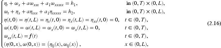
To prove the well-posedness result for system (1.4), we consider the nonhomogeneous system

{\begin{cases} η_{t} + ω_{x} + a ω_{x x x} + a_{1} ω_{x x x x x} = h_{1}, & in (0, T) \times (0, L), \\ ω_{t} + η_{x} + a η_{x x x} + a_{1} η_{x x x x x} = h_{2}, & in (0, T) \times (0, L), \\ η (t, 0) = η (t, L) = η_{x} (t, 0) = η_{x} (t, L) = η_{x x} (t, 0) = 0, & t \in (0, T), \\ ω (t, 0) = ω (t, L) = ω_{x} (t, 0) = ω_{x} (t, L) = 0, & t \in (0, T), \\ ω_{x x} (t, L) = f (t) & t \in (0, T), \\ (η (0, x), ω (0, x)) = (η_{0} (x), ω_{0} (x)), & x \in (0, L), \end{cases}

(2.16)

where the parameters

a, a_{1}

verify (1.3). Remember the definition of

X_{3}

given by (1.7), and also consider the following set:

{\tilde{X}}_{3} := {(φ, ψ) \in {[H^{3} (0, L) \cap H_{0}^{2} (0, L)]}^{2} | φ_{x x} (0) = ψ_{x x} (L) = 0} .

We define a solution by transposition as follows, see Lions and Magenes (1968, 1986), to justify the choice of formula (2.17) below:

Definition 1 (Solution by transposition)

Let $T > 0,$ $(η_{0}, ω_{0}) \in X_{3}$ , $f \in L^{2} (0, T)$ and

(h_{1}, h_{2}) \in L^{2} (0, T, [H^{- 2} (0, L)]^{2}) .

A solution of problem (2.16) is a function

(η, ω) \in C (0, T; X_{3})

such that, for all

σ \in [0, T]

and

(φ_{σ}, ψ_{σ}) \in {\tilde{X}}_{3}

the following identity holds

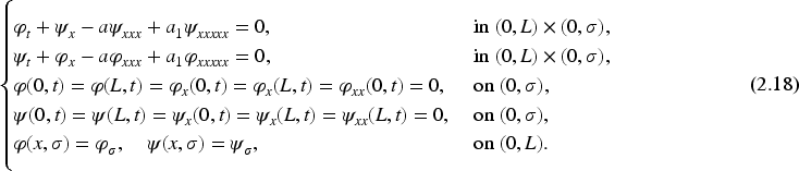
\begin{aligned} {⟨ (η (σ), ω (σ)), (φ_{σ}, ψ_{σ}) ⟩}_{[H^{3} (0, L) \cap H_{0}^{2} (0, L)]^{2}} = {⟨ (η_{0}, ω_{0}), (φ (0), ψ (0)) ⟩}_{[H^{3} (0, L) \cap H_{0}^{2} (0, L)]^{2}} \\ + \int_{0}^{σ} f (t) φ_{x x} (t, L) d t + \int_{0}^{σ} {⟨ (h_{1} (t), h_{2} (t)), (φ (t), ψ (t)) ⟩}_{(H^{- 2}, H_{0}^{2})^{2}} d t, \end{aligned}

(2.17)

where the pair

(φ, ψ)

is the solution of

{\begin{cases} φ_{t} + ψ_{x} - a ψ_{x x x} + a_{1} ψ_{x x x x x} = 0, & in (0, L) \times (0, σ), \\ ψ_{t} + φ_{x} - a φ_{x x x} + a_{1} φ_{x x x x x} = 0, & in (0, L) \times (0, σ), \\ φ (0, t) = φ (L, t) = φ_{x} (0, t) = φ_{x} (L, t) = φ_{x x} (0, t) = 0, & on (0, σ), \\ ψ (0, t) = ψ (L, t) = ψ_{x} (0, t) = ψ_{x} (L, t) = ψ_{x x} (L, t) = 0, & on (0, σ), \\ φ (x, σ) = φ_{σ}, ψ (x, σ) = ψ_{σ}, & on (0, L) . \end{cases}

(2.18)

Thanks to Capistrano-Filho et al. (2019, Corollary 2.5 and Proposition 2.6), the following well-posedness result for system (2.18) is established:

Proposition 2.6

For all $(φ_{σ}, ψ_{σ}) \in {\tilde{X}}_{3},$ system (2.18) admits a unique solution $(φ, ψ) \in C ([0, σ]; {\tilde{X}}_{3}),$ which satisfies

‖ (φ (t), ψ (t)) ‖_{[H^{3} (0, L) \cap H_{0}^{2} (0, L)]^{2}} \leq C ‖ (φ_{σ}, ψ_{σ}) ‖_{[H^{3} (0, L) \cap H_{0}^{2} (0, L)]^{2}}, \forall t \in [0, σ] .

(2.19)

Additionally, we have that

\int_{0}^{σ} | φ_{x x} (L, t) |^{2} + | ψ_{x x} (0, t) |^{2} d t \leq C ‖ (φ_{σ}, ψ_{σ}) ‖_{[H_{0}^{2} (0, L)]^{2}}^{2} .

(2.20)

The following result gives us the existence and uniqueness of the solution for system (2.16).

Lemma 2.7

Let $T > 0, (η_{0}, ω_{0}) \in X_{3}, (h_{1}, h_{2}) \in L^{2} (0, T; [H^{- 2} (0, L)]^{2})$ and $f \in L^{2} (0, T)$ . There exists a unique solution $(η, ω) \in C ([0, T]; X_{3})$ of system (2.16). Moreover, there exists a positive constant $C_{T}$ , such that

\begin{aligned} ‖ (η (σ), ω (σ)) ‖_{[H^{3} (0, L) \cap H_{0}^{2} (0, L)]^{2}} & \leq C_{T} ({‖ (η_{0}, ω_{0}) ‖}_{[H^{3} (0, L) \cap H_{0}^{2} (0, L)]^{2}} + ‖ f ‖_{L^{2} (0, T)} {‖ (h_{1}, h_{2}) ‖}_{L^{2} (0, T : [H_{0}^{2} (0, L)]^{2})}), \end{aligned}

(2.21)

for all

σ \in [0, T]

Proof.

Let us define $Δ$ as the linear functional given by the right-hand side of (2.17), that is

\begin{aligned} Δ (φ_{σ}, ψ_{σ}) = & {⟨ (η_{0}, ω_{0}), (φ (0), ψ (0)) ⟩}_{[H^{3} (0, L) \cap H_{0}^{2} (0, L)]^{2}} + \int_{0}^{σ} f (t) φ_{x x} (t, L) d t \\ + \int_{0}^{σ} {⟨ (h_{1} (t), h_{2} (t)), (φ (t), ψ (t)) ⟩}_{(H^{- 2}, H_{0}^{2})^{2}} d t . \end{aligned}

We infer from (2.19), (2.20), and the Cauchy–Schwarz inequality that

\begin{aligned} | Δ (φ_{σ}, ψ_{σ}) | \leq & ‖ (η_{0}, ω_{0}) ‖_{[H^{3} (0, L) \cap H_{0}^{2} (0, L)]^{2}} ‖ (φ_{σ}, ψ_{σ}) ‖_{[H^{3} (0, L) \cap H_{0}^{2} (0, L)]^{2}} + ‖ f ‖_{L^{2} (0, T)} ‖ φ_{x x} (L) ‖_{L^{2} (0, T)} \\ + C ‖ (φ_{σ}, ψ_{σ}) ‖_{[H^{3} (0, L) \cap H_{0}^{2} (0, L)]^{2}} ‖ (h_{1}, h_{2}) ‖_{L^{1} (0, T : H^{- 2} (0, L)} \\ \leq & C_{T} (‖ (η_{0}, ω_{0}) ‖_{[H^{3} (0, L) \cap H_{0}^{2} (0, L)]^{2}} + ‖ f ‖_{L^{2} (0, T)} + ‖ (h_{1}, h_{2}) ‖_{L^{1} (0, T : H^{- 2} (0, L)}) ‖ (φ_{σ}, ψ_{σ}) ‖_{[H^{3} (0, L) \cap H_{0}^{2} (0, L)]^{2}}, \end{aligned}

and we obtain that

Δ \in L ([H^{3} (0, L) \cap H_{0}^{2} (0, L)]^{2}; R) .

Thus, from the Riesz-representation theorem, there exists one and only one

(η_{σ}, ω_{σ}) \in [H^{3} (0, L) \cap H_{0}^{2} (0, L)]^{2}

such that

{\begin{cases} Δ (φ_{σ}, ψ_{σ}) = {⟨ (η_{σ}, ω_{σ}), (φ_{σ}, ψ_{σ}) ⟩}_{[H^{3} (0, L) \cap H_{0}^{2} (0, L)]^{2}} \\ with ‖ Δ ‖_{L ([H^{3} (0, L) \cap H_{0}^{2} (0, L)]^{2}; R)} = ‖ (η_{σ}, ω_{σ}) ‖_{[H^{3} (0, L) \cap H_{0}^{2} (0, L)]^{2}}, \end{cases}

(2.22)

and we obtain the uniqueness of the solution to problem (2.16). Now, in order to prove the estimate (2.21), we define the map

(η, ω) : [0, T] \to [H^{3} (0, L) \cap H_{0}^{2} (0, L)]^{2}

(η (σ), ω (σ)) := (η_{σ}, ω_{σ}) for all σ \in [0, T],

and we conclude from (2.22) that

\begin{aligned} ‖ (η (σ), ω (σ)) ‖_{[H^{3} (0, L) \cap H_{0}^{2} (0, L)]^{2}} = & ‖ Δ ‖_{L ([H^{3} (0, L) \cap H_{0}^{2} (0, L)]^{2}; R)} \\ \leq & C_{T} ({‖ (η_{0}, ω_{0}) ‖}_{[H^{3} (0, L) \cap H_{0}^{2} (0, L)]^{2}} + ‖ f ‖_{L^{2} (0, T)} + {‖ (h_{1}, h_{2}) ‖}_{L^{2} (0, T : [H_{0}^{2} (0, L)]^{2})}) . \end{aligned}

Finally, the fact that

(η, ω) \in C ([0, T]; X_{3})

was already proved in Capistrano-Filho and Gallego (2018) and Capistrano-Filho et al. (2019), and hence we omit the details.

Now, we pass to show the well-posedness of the nonhomogeneous feedback linear system associated with (2.16)

Lemma 2.8

Let $T > 0$ . Then, for every $(η_{0}, ω_{0})$ in $X_{3}$ and $(h_{1}, h_{2})$ in $L^{2} (0, T; [H^{- 2} (0, L)]^{2})$ , there exists a unique solution $(η, ω)$ of system (2.16) such that $(η, ω) \in C ([0, T]; X_{3}),$ with $f (t) = α η_{x x} (t, L) + β η_{x x} (t - τ (t), L)$ , where $α$ and $β$ belong to $R$ . Moreover, for some positive constant $C = C (T)$ , we have

‖ (η (t), ω (t)) ‖_{[H^{3} (0, L) \cap H_{0}^{2} (0, L)]^{2}} \leq C ({‖ (η_{0}, ω_{0}) ‖}_{[H^{3} (0, L) \cap H_{0}^{2} (0, L)]^{2}} + {‖ (h_{1}, h_{2}) ‖}_{L^{2} (0, T; [H^{- 2} (0, L)]^{2})}),

for all

t \in [0, T] .

Proof.

Note that if $(η, ω) \in C ([0, T]; X_{3}),$ from the trace theorems, it follows that

f (t) = α η_{x x} (t, L) + β η_{x x} (t - τ (t), L) \in L^{2} (0, T) .

We claim that: there exists a positive constant $C_{α, β}$ such that

‖ f ‖_{L^{2} (0, T)} \leq C_{α, β} T^{1 / 2} ‖ (η, ω) ‖_{C ([0, T]; [H^{3} (0, L) \cap H_{0}^{2} (0, L)]^{2})} .

(2.23)

Indeed, note that

\begin{aligned} ‖ f ‖_{L^{2} (0, T)}^{2} & \leq | α |^{2} C T ‖ η ‖_{C ([0, T]; H^{3} (0, L))}^{2} + | β |^{2} \int_{0}^{T} | η (t - τ (t), L) |^{2} d t \\ \leq | α |^{2} C T | η ‖_{C ([0, T]; H^{3} (0, L))}^{2} + | β |^{2} \int_{0}^{T - τ (T)} | η (s, L) |^{2} \frac{1}{1 - \dot{τ} (t)} d s . \end{aligned}

By using the conditions in (1.5), we deduce the existence of some positive constant

C_{M}

such that

‖ f ‖_{L^{2} (0, T)}^{2} \leq (| α |^{2} C + | β |^{2} \frac{C_{M}}{1 - d}) T ‖ η ‖_{C ([0, T]; H^{3} (0, L))}^{2},

giving the claim.

Now, let $0 < γ \leq T$ to be determined later. For each $(η_{0}, ω_{0}) \in X_{3},$ consider the map

\begin{aligned} Γ : C ([0, γ]; [H^{3} (0, L) \cap H_{0}^{2} (0, L)]^{2}) & ⟶ C ([0, γ]; [H^{3} (0, L) \cap H_{0}^{2} (0, L)]^{2}) \\ (η, ω) & ⟼ Γ (η, ω) = (w, v), \end{aligned}

where

(w, v)

is the solution of (2.16) with

f (t) = α η_{x x} (t, L) + β η_{x x} (t - τ (t), L) .

By Lemma 2.7 and (2.23), the linear operator

Γ

is well defined. Furthermore, there exists a positive constant

C_{γ}

such that

\begin{aligned} ‖ Γ (η, ω) ‖_{C ([0, γ]; [H^{3} (0, L) \cap H_{0}^{2} (0, L)]^{2})} \leq & C_{γ} ({‖ (η_{0}, ω_{0}) ‖}_{[H^{3} (0, L) \cap H_{0}^{2} (0, L)]^{2}} + {‖ (h_{1}, h_{2}) ‖}_{L^{2} (0, γ : [H^{- 2} (0, L)]^{2})} \\ + ‖ α η_{x x} (L) + β η_{x x} (\cdot - τ (\cdot), L) ‖_{L^{2} (0, γ)}) . \end{aligned}

From (2.23), it follows that

\begin{aligned} ‖ Γ (η, ω) ‖_{C ([0, γ]; [H^{3} (0, L) \cap H_{0}^{2} (0, L)]^{2})} \leq & C_{γ} ({‖ (η_{0}, ω_{0}) ‖}_{[H^{3} (0, L) \cap H_{0}^{2} (0, L)]^{2}} + {‖ (h_{1}, h_{2}) ‖}_{L^{2} (0, γ : [H^{- 2} (0, L)]^{2})}) \\ + C_{α, β} γ^{1 / 2} ‖ (η, ω) ‖_{C ([0, T]; [H^{3} (0, L) \cap H_{0}^{2} (0, L)]^{2})} . \end{aligned}

Let

(η, ω) \in B_{R} (0),

where

B_{R} (0) := {(η, ω) \in C ([0, γ]; [H^{3} (0, L) \cap H_{0}^{2} (0, L)]^{2}) : ‖ (η, ω) ‖_{C ([0, γ]; [H^{3} (0, L) \cap H_{0}^{2} (0, L)]^{2})} \leq R},

and

R = 2 C_{T} ({‖ (η_{0}, ω_{0}) ‖}_{[H^{3} (0, L) \cap H_{0}^{2} (0, L)]^{2}} + {‖ (h_{1}, h_{2}) ‖}_{L^{2} (0, T : [H^{- 2} (0, L)]^{2})}) .

Choosing

γ

such that

C_{α, β} γ^{1 / 2} \leq \frac{1}{2},

it follows that

‖ Γ (η, ω) ‖_{C ([0, γ]; [H^{3} (0, L) \cap H_{0}^{2} (0, L)]^{2})} \leq R,

and

\begin{aligned} ‖ Γ (η_{1}, ω_{1}) - Γ (η_{2}, ω_{2}) ‖_{C ([0, γ]; [H^{3} (0, L) \cap H_{0}^{2} (0, L)]^{2})} \leq \frac{1}{2} ‖ (η_{1}, ω_{1}) - (η_{2}, ω_{2}) ‖_{C ([0, γ]; [H^{3} (0, L) \cap H_{0}^{2} (0, L)]^{2})} . \end{aligned}

Hence,

Γ : B_{R} (0) \to B_{R} (0)

is a contraction, and by Banach Fixed Point Theorem, we obtain a unique

(η, ω) \in B_{R} (0)

such that

Γ (η, ω) = (η, ω)

and

\begin{aligned} ‖ (η, ω) ‖_{C ([0, γ]; [H^{3} (0, L) \cap H_{0}^{2} (0, L)]^{2})} & \leq 2 C_{T} ({‖ (η_{0}, ω_{0}) ‖}_{[H^{3} (0, L) \cap H_{0}^{2} (0, L)]^{2}} + {‖ (h_{1}, h_{2}) ‖}_{L^{2} (0, T : [H^{- 2} (0, L)]^{2})}) . \end{aligned}

Since

γ

is independent of

(η_{0}, ω_{0}),

the standard continuation extension argument yields that the solution

(η, ω)

belongs to

C ([0, T]; [H^{3} (0, L) \cap H_{0}^{2} (0, L)]^{2}),

and the proof ends.

The first main result of the article ensures the existence of local solutions to (1.4) and is proved below.

Proof of Theorem 1.1. Proof of Theorem 1.1.

Let $T > 0$ and $‖ (η_{0}, ω_{0}) ‖_{[H^{3} (0, L) \cap H_{0}^{2} (0, L)]^{2}} < θ,$ where $θ > 0$ will be determined later. We know from Capistrano-Filho et al. (2019) that for $(η, ω) \in C ([0, T]; [H^{3} (0, L) \cap H_{0}^{2} (0, L)]^{2}),$ there exists a positive constant $C_{1}$ such that the following inequalities hold true:

\begin{aligned} ‖ η ω_{x} ‖_{L^{2} (0, T; L^{2} (0, L))} & \leq C_{1} T^{1 / 2} ‖ (η, ω) ‖_{C (0, T; [H^{3} (0, L) \cap H_{0}^{2} (0, L)]^{2})}^{2}, \end{aligned}

\begin{aligned} ‖ η_{x} ω_{x x} ‖_{L^{2} (0, T; L^{2} (0, L))} & \leq C_{1} T^{1 / 2} ‖ (η, ω) ‖_{C (0, T; [H^{3} (0, L) \cap H_{0}^{2} (0, L)]^{2})}^{2}, \end{aligned}

and

‖ η ω_{x x x} ‖_{L^{2} (0, T; L^{2} (0, L))} \leq C_{1} T^{1 / 2} ‖ (η, ω) ‖_{C (0, T; [H^{3} (0, L) \cap H_{0}^{2} (0, L)]^{2})}^{2} .

Thus, the nonlinearities

(h_{1}, h_{2}) := (- (η ω)_{x} - α^{'} (η ω_{x x})_{x}, - ω ω_{x} - c (ω ω_{x})_{x x} - (η η_{x x})_{x} + β^{'} ω_{x} ω_{x x} + ρ ω ω_{x x x})

belong to

L^{2} (0, T; [L^{2} (0, L)]^{2}),

and

{\begin{cases} ‖ h_{1} ‖_{L^{2} (0, T; L^{2} (0, L))} \leq (2 + 2 | α^{'} |) C_{1} T^{1 / 2} ‖ (η, ω) ‖_{C (0, T; [H^{3} (0, L) \cap H_{0}^{2} (0, L)]^{2})}^{2}, \\ ‖ h_{2} ‖_{L^{2} (0, T; L^{2} (0, L))} \leq (3 + 4 | c | + | β^{'} | + | ρ |) C_{1} T^{1 / 2} ‖ (η, ω) ‖_{C (0, T; [H^{3} (0, L) \cap H_{0}^{2} (0, L)]^{2})}^{2} . \end{cases}

(2.24)

Taking this into consideration, we define the following map:

\begin{aligned} Γ : C ([0, T]; {[H^{3} (0, L) \cap H_{0}^{2} (0, L)]}^{2}) & ⟶ C ([0, T]; {[H^{3} (0, L) \cap H_{0}^{2} (0, L)]}^{2}) \\ (η, ω) & ⟼ Γ (η, ω) = (\bar{η}, \bar{ω}), \end{aligned}

where

(\bar{η}, \bar{ω})

is the solution of (2.16) with

(h_{1}, h_{2}) \in L^{2} (0, T; [L^{2} (0, L)]^{2}) \subset L^{2} (0, T; [H^{- 2} (0, L)]^{2}),

as defined above, and with

f (t) = α η_{x x} (t, L) + β η_{x x} (t - τ (t), L) .

From Lemma 2.8, we find that

Γ

is well defined and there exists a positive constant

C_{T}

such that

\begin{aligned} ‖ Γ (η, ω) ‖_{C ([0, T] : [H^{3} (0, L) \cap H_{0}^{2} (0, L)]^{2})} & \leq C_{T} ({‖ (η_{0}, ω_{0}) ‖}_{[H^{3} (0, L) \cap H_{0}^{2} (0, L)]^{2}} + {‖ (h_{1}, h_{2}) ‖}_{L^{2} (0, T : [H_{0}^{2} (0, L)]^{2})}) . \end{aligned}

On the other hand, from the inequalities (2.24), we have that

\begin{aligned} ‖ Γ (η, ω) ‖_{C ([0, T] : [H^{3} (0, L) \cap H_{0}^{2} (0, L)]^{2})} & \leq C_{T} {‖ (η_{0}, ω_{0}) ‖}_{[H^{3} (0, L) \cap H_{0}^{2} (0, L)]^{2}} + C_{T} 13 K C_{1} T^{1 / 2} ‖ (η, ω) ‖_{C ([0, T] : [H^{3} (0, L) \cap H_{0}^{2} (0, L)]^{2})}^{2}, \end{aligned}

(2.25)

where

K = max {1, | c |, | α^{'} |, | β^{'} |, | ρ |} .

Now, we consider the ball

B_{R} (0) = {(η, ω) \in C ([0, T] : [H^{3} (0, L) \cap H_{0}^{2} (0, L)]^{2}) : ‖ (η, ω) ‖_{C ([0, T] : [H^{3} (0, L) \cap H_{0}^{2} (0, L)]^{2})} \leq R},

with

R = 2 C_{T} ‖ (η_{0}, ω_{0}) ‖_{[H^{3} (0, L) \cap H_{0}^{2} (0, L)]^{2}} .

The inequality (2.25) leads to

‖ Γ (η, ω) ‖_{C ([0, T] : [H^{3} (0, L) \cap H_{0}^{2} (0, L)]^{2})} \leq \frac{R}{2} + C_{T} 13 K C_{1} T^{1 / 2} R^{2} \leq \frac{R}{2} + C_{T}^{2} 26 K C_{1} T^{1 / 2} θ R,

for all

(η, ω) \in B_{R} (0) .

By choosing

θ

such that

C_{T}^{2} 26 K C_{1} T^{1 / 2} θ < \frac{1}{4},

we obtain that

Γ (B_{R} (0)) \subset B_{R} (0) .

Finally, following the same argument as done in Lemma 2.8, we can conclude that

Γ

is a contraction in

B_{R} (0)

, then, the Banach Fixed Point Theorem guarantees the existence of a unique

(η, ω) \in B_{R} (0)

such that

Γ (η, ω) = (η, ω)

and

‖ (η, ω) ‖_{C ([0, T] : [H^{3} (0, L) \cap H_{0}^{2} (0, L)]^{2})} \leq 2 C_{T} {‖ (η_{0}, u_{0}) ‖}_{[H^{3} (0, L) \cap H_{0}^{2} (0, L)]^{2}},

achieving the proof.

Remark 1

In (1.5), the time-dependent delay is assumed to be positive for all $t \geq 0$ . This requirement is relaxed in Nicaise et al. (2011) since $τ$ is allowed to degenerate. Notwithstanding, the problem in Nicaise et al. (2011) is linear and hence simpler than ours. The key idea of the proof in Nicaise et al. (2011) is to consider a new delay $τ_{ϵ}$ defined by

τ_{ϵ} (t) := ϵ + τ_{ϵ} (t),

where

0 < ϵ < \bar{ϵ}

, for some

\bar{ϵ} > 0

. Therefore,

τ_{ϵ}

satisfy (1.5) and hence problem (2.1) has a unique solution

U_{ϵ}

. The whole task is to tend

ϵ

0

under more regularity on the solution. We have tried to adopt this approach, but we faced difficulties because of the nonlinearities in our problem.

3. Long-Time Behavior of Solutions

In this section, we are in a position to prove the second main result of our work. First, we demonstrate that the energy associated with (1.9) is exponentially stable. Moreover, we establish that the solutions decay at an optimal rate.

3.1. Proof of Theorem 1.2

Recall that Theorem 2.2 (see also Proposition 2.3) guarantees the $L^{2}$ a priori estimate for the linear system (2.1) whose operator is defined by (2.3)–(2.4). Therefore, the solutions of system (1.9) are globally well-posed. Whereupon, we can treat the exponential stability for this system.

To proceed, consider the following Lyapunov functional

V (t) = E (t) - μ_{1} V_{1} (t) + μ_{2} V_{2} (t),

where

μ_{1}, μ_{2} \in R^{+}

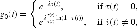
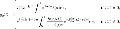
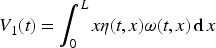
will be chosen later. Here,

E (t)

is the total energy given by (1.8), while

V_{1} (t) = \int_{0}^{L} x η (t, x) ω (t, x) d x

and

V_{2} (t) = \frac{| β |}{2} τ (t) \int_{0}^{1} (1 - ρ) η_{x x}^{2} (t - τ (t) ρ, L) d ρ .

Observe that,

(1 - max {μ_{1} L, μ_{2}}) E (t) \leq V (t) \leq (1 + max {μ_{1} L, μ_{2}}) E (t),

(3.1)

by assuming

0 < μ_{1} < 1 / L

and

0 < μ_{2} < 1

On the other hand, using system (1.9) and the boundary conditions, we get that

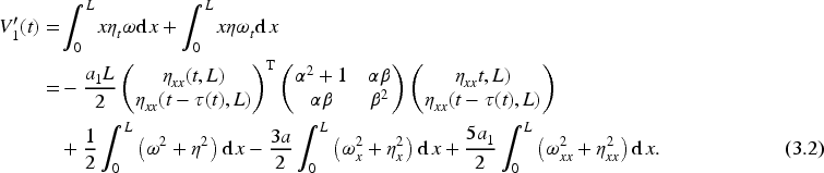
\begin{aligned} V_{1}^{'} (t) = & \int_{0}^{L} x η_{t} ω d x + \int_{0}^{L} x η ω_{t} d x \\ = & - \frac{a_{1} L}{2} {(\begin{matrix} η_{x x} (t, L) \\ η_{x x} (t - τ (t), L) \end{matrix})}^{T} (\begin{matrix} α^{2} + 1 & α β \\ α β & β^{2} \end{matrix}) (\begin{matrix} η_{x x} t, L) \\ η_{x x} (t - τ (t), L) \end{matrix}) \\ + \frac{1}{2} \int_{0}^{L} (ω^{2} + η^{2}) d x - \frac{3 a}{2} \int_{0}^{L} (ω_{x}^{2} + η_{x}^{2}) d x + \frac{5 a_{1}}{2} \int_{0}^{L} (ω_{x x}^{2} + η_{x x}^{2}) d x . \end{aligned}

(3.2)

In addition, from (2.2) and by integration by parts, we deduce that

V_{2}^{'} (t) = - \frac{| β |}{2} \int_{0}^{1} (1 - \dot{τ} (t) ρ) η_{x x}^{2} (t - τ (t) ρ, L) d ρ + \frac{| β |}{2} η_{x x}^{2} (t, L) .

(3.3)

Thus, from (2.7), (3.2), and (3.3), we have that

V^{'} (t) + λ V (t) = S_{1} + S_{2} + S_{3},

(3.4)

where

S_{1} = \frac{1}{2} ⟨ Ψ_{μ_{1}, μ_{2}} (η_{x x} (t, L), η_{x x} (t - τ (t), L)), (η_{x x} (t, L), η_{x x} (t - τ (t), L)) ⟩,

with (recall (1.6))

\begin{aligned} Ψ_{μ_{1}, μ_{2}} & = Φ_{α, β} + \frac{a_{1} L μ_{1}}{2} (\begin{matrix} α^{2} + 1 & α β \\ α β & β^{2} \end{matrix}) + \frac{| β | μ_{2}}{2} (\begin{matrix} 1 & 0 \\ 0 & 0 \end{matrix}), \end{aligned}

\begin{aligned} S_{2} & = - \frac{μ_{1}}{2} \int_{0}^{L} (ω^{2} + η^{2}) d x + \frac{3 a μ_{1}}{2} \int_{0}^{L} (ω_{x}^{2} + η_{x}^{2}) d x + \frac{λ}{2} \int_{0}^{L} (η^{2} + ω^{2}) d x \\ + μ_{1} λ \int_{0}^{L} x η ω d x - \frac{5 a_{1} μ_{1}}{2} \int_{0}^{L} (ω_{x x}^{2} + η_{x x}^{2}) d x, \end{aligned}

and

\begin{aligned} S_{3} & = - μ_{2} \frac{| β |}{2} \int_{0}^{1} (1 - \dot{τ} (t) ρ) η_{x x}^{2} (t - τ (t) ρ, L) d ρ + \frac{λ | β |}{2} τ (t) \int_{0}^{1} η_{x x}^{2} (t - τ (t) ρ, L) d ρ \\ + \frac{μ_{2} | β | λ}{2} τ (t) \int_{0}^{1} (1 - ρ) η_{x x}^{2} (t - τ (t) ρ, L) d ρ, \end{aligned}

respectively.

The objective is to show that $V^{'} (t) + λ V (t) \leq 0$ . To do so, let us deal with each term $S_{i}$ in (3.4), for $i = 1, 2, 3$ .

Estimate of $S_{1}$ : Since the matrix $Φ_{α, β}$ (see (1.6)) is negative definite, it follows from the continuity of the trace and determinant functions that one can choose $μ_{1}, μ_{2} \in (0, 1)$ sufficiently small so that the new matrix $Ψ_{μ_{1}, μ_{2}}$ is also negative definite. Thus,

S_{1} \leq 0.

Estimate of $S_{2}$ : Observe that using Poincaré inequality, we get

\begin{aligned} S_{2} \leq & \frac{L^{2}}{2 π^{2}} λ (1 + μ_{1} L) \int_{0}^{L} (ω_{x}^{2} + η_{x}^{2}) d x + \frac{3 a μ_{1}}{2} \int_{0}^{L} (ω_{x}^{2} + η_{x}^{2}) d x - \frac{5 a_{1} μ_{1}}{2} \int_{0}^{L} (ω_{x x}^{2} + η_{x x}^{2}) d x \\ \leq & [\frac{L^{2}}{2 π^{2}} (λ (1 + μ_{1} L) \frac{L^{2}}{2 π^{2}} + 3 a μ_{1}) - \frac{5 a_{1} μ_{1}}{2}] \int_{0}^{L} (ω_{x x}^{2} + η_{x x}^{2}) d x . \end{aligned}

Thus,

S_{2} < 0,

\begin{aligned} λ < \frac{μ_{1} π^{2} (5 a_{1} π^{2} - 3 a L^{2})}{L^{4} (1 + μ_{1})} . \end{aligned}

Estimate of $S_{3}$ : We proceed as in Capistrano-Filho et al. (2024), choosing

λ < \frac{μ_{2} (1 - d)}{M (1 + μ_{2})},

it follows that

S_{3} < 0.

Therefore, for the estimates above, we have

\frac{d}{d t} V (t) + λ V (t) \leq 0,

and, since

V (t)

satisfies (3.1), we deduce that

E (t) \leq ζ E (0) e^{- λ t}, \forall t \geq 0,

for

ζ > 0

and

λ > 0

fulfilling (1.10) and (1.11), respectively. This achieves the proof of the theorem. □

3.2. Decay Rate: An Optimal Result

We can optimize the value of $λ$ in Theorem 1.2 to obtain the best decay rate for the linear system (1.9) in the following way:

Proposition 3.1
If the constant $μ_{1}$ given in Theorem 1.2 is chosen as follows:
$μ_{1} \in [0, \frac{(2 a_{1} α - | β |) (1 - d) - a_{1}^{2} | β |}{L (1 - d) (a_{1}^{2} + α^{2})}),$
(3.5)
then $λ$ has the largest possible value.
Proof.
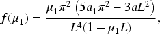
Define the functions $f$ and
$g : [0, \frac{(2 a_{1} α - | β |) (1 - d) - a_{1}^{2} | β |}{L (1 - d) (a_{1}^{2} + α^{2})}] \to R$
by
$f (μ_{1}) = \frac{μ_{1} π^{2} (5 a_{1} π^{2} - 3 a L^{2})}{L^{4} (1 + μ_{1} L)},$
and
$g (μ_{1}) = \frac{(2 a_{1} α - | β |) (1 - d) - a_{1}^{2} | β | - L (1 - d) (a_{1}^{2} + α^{2}) μ_{1}}{M (2 a_{1} α (1 - d) - a_{1}^{2} | β | - L (1 - d) (a_{1}^{2} + α^{2}) μ_{1})} (1 - d),$
respectively. On the other hand, let us consider $λ (μ_{1}) = min {f (μ_{1}), g (μ_{1})}$ . Thus, we have the following claims. Claim 2
The function $f$ (respectively, $g$ ) is increasing (respectively, decreasing) in the interval
$[0, \frac{(2 a_{1} α - | β |) (1 - d) - a_{1}^{2} | β |}{L (1 - d) (a_{1}^{2} + α^{2})}) .$

A simple computation shows that
$f^{'} (μ_{1}) > 0, for all μ_{1} \geq 0$
and hence $f^{'} (μ_{1}) > 0$ for
$μ_{1} \in [0, \frac{(2 a_{1} α - | β |) (1 - d) - a_{1}^{2} | β |}{L (1 - d) (a_{1}^{2} + α^{2})}) .$

Furthermore, one can rewrite $g$ as follows:
$\begin{aligned} g (μ_{1}) & = \frac{1 - d}{M} - \frac{| β | (1 - d)^{2}}{M L (1 - d) (a_{1}^{2} + α^{2})} (\frac{1}{\frac{2 a_{1} α (1 - d) - a_{1}^{2} | β |}{L (1 - d) (a_{1}^{2} + α^{2})} - μ_{1}}), \end{aligned}$
and thus
$\begin{aligned} g^{'} (μ_{1}) & = - \frac{| β | (1 - d)^{2}}{M L (1 - d) (a_{1}^{2} + α^{2})} [\frac{1}{{(\frac{2 a_{1} α (1 - d) - a_{1}^{2} | β |}{L (1 - d) (a_{1}^{2} + α^{2})} - μ_{1})}^{2}}] < 0. \end{aligned}$
This ascertains the Claim 2. Claim 3
There exists only one point $μ_{1}$ , satisfying (3.5) such that $f (μ_{1}) = g (μ_{1})$ .
Indeed, since
$f (0) = 0, f (\frac{(2 a_{1} α - | β |) (1 - d) - a_{1}^{2} | β |}{L (1 - d) (a_{1}^{2} + α^{2})}) > 0,$
and
$g (0) > 0, g (\frac{(2 a_{1} α - | β |) (1 - d) - a_{1}^{2} | β |}{L (1 - d) (a_{1}^{2} + α^{2})}) = 0,$
the existence of this point is a direct consequence of the mean value theorem, applied to the function $F = f - g$ . The uniqueness follows from the fact that the function $F = f - g$ is increasing in this interval, and Claim 3 holds.

Lastly, thanks to the Claims 2 and 3, the maximum value of the function $λ$ is obtained when $μ_{1}$ satisfies (3.5), where $f (μ_{1}) = g (μ_{1})$ , and the proof of Proposition 3.1 is achieved.
4. Conclusion

This paper establishes the existence and uniqueness of a solution for a higher-order nonlinear Boussinesq system in a bounded domain, even when a time-dependent delay is present in one of the boundary conditions. Additionally, we prove that solutions to the linearized problem are exponentially stable, both results being obtained under certain conditions related to the system’s parameters and the delay. These findings extend the results of the second and third authors in Capistrano-Filho et al. (2024) for a higher-order dispersive system. Further comments on our results are provided below. (1)

It is worth mentioning that the solutions of system (1.4) obtained in Theorem 1.1 are local. Proving the global existence of solutions remains a challenge due to the absence of an a priori $L^{2}$ estimate. Specifically, it is challenging to tackle this problem within the energy space for the nonlinear system that includes a delay term.

(2)

Observe that the restriction $0 < L < \sqrt{(5 a_{1} / 3 a)} π$ in Theorem 1.2 arises from the Kato smoothing effect, which does not occur in the lower-order Boussinesq system (see, e.g., Capistrano-Filho et al., 2024). This difference is because in system (1.4), we have spatial derivatives of order three and five, both with positive signs. Thus, after performing some integration by parts, the left-hand side of (2.14) contains the $H^{1}$ -norm with a negative sign and the $H^{2}$ -norm with a positive sign. To recover the $H^{2}$ -norm, the Poincaré inequality must be applied, which imposes this restriction on the size of $L$ .

(3)

A version of the higher-order Boussinesq system was proposed by Olver (1984, equations (4.7) and (4.8), p. 283) and is given by:

{\begin{cases} η_{t} + u_{x} + \frac{1}{6} β (3 θ^{2} - 1) u_{x x x} + \frac{1}{120} β^{2} (25 θ^{4} - 10 θ^{2} + 1) u_{x x x x x} \\ + α (η u)_{x} + \frac{1}{2} α β (θ^{2} - 1) {(η u_{x x})}_{x} = 0, \\ u_{t} + η_{x} + β [\frac{1}{2} (1 - θ^{2}) - τ] η_{x x x} + β^{2} [\frac{1}{24} (θ^{4} - 6 θ^{2} + 5) + \frac{τ}{2} (θ^{2} - 1)] η_{x x x x x} \\ + α u u_{x} + α β [{(η η_{x x})}_{x} + (2 - θ^{2}) u_{x} u_{x x}] = 0. \end{cases}

Through scaling, we arrive at the following system:

{\begin{cases} η_{t} + u_{x} - a u_{x x x} + a_{1} (η u)_{x} + a_{2} {(η u_{x x})}_{x} + b u_{x x x x x} = 0, & in (0, L) \times (0, \infty), \\ u_{t} + η_{x} - a η_{x x x} + a_{1} u u_{x} + a_{3} {(η η_{x x})}_{x} + a_{4} u_{x} u_{x x} + b η_{x x x x x} = 0, & in (0, L) \times (0, \infty), \\ η (x, 0) = η_{0} (x), u (x, 0) = u_{0} (x), & in (0, L), \end{cases}

(4.1)

where

a > 0, b > 0, a \neq b, a_{1} > 0, a_{2} < 0, a_{3} > 0

and

a_{4} > 0

. System (4.1) was studied in Capistrano-Filho et al. (2019). Using the same boundary conditions as in problem (1.4), we believe that similar results proved in our work can be obtained for system (4.1) without the restriction over

L

since the sign of the third derivatives in (4.1) is negative instead of positive unlike our case (see system (1.4)).

(4)

It is important to point out that system (1.4) is shown to be locally well-posed, and hence we are unable to establish any exponential stability for the nonlinear problem. One interesting research avenue is to show the stability for the nonlinear problem.

Footnotes

Acknowledgments

The authors are grateful to the associate editor and the referees for the careful reading of this paper and their valuable suggestions and comments.

Funding

The authors disclosed receipt of the following financial support for the research, authorship, and/or publication of this article: Roberto de A Capistrano-Filho was partially supported by CAPES/COFECUB grant number 88887.879175/2023-00, CNPq grant numbers 421573/2023-6 and 307808/2021-1, and Propesqi - QUALIS A (UFPE). George J Bautista was supported by Universidad Tecnológica de los Andes, Abancay-Peru. Oscar Sierra Fonseca was supported by FAPERJ (Rio de Janeiro, Brazil) grant number SEI 260003/000175/2024 and by Escola de Matemática Aplicada, Fundação Getúlio Vargas (Rio de Janeiro - Brazil).

Declaration of Conflicting Interests

The authors declared no potential conflicts of interest with respect to the research, authorship, and/or publication of this article.

Data Availability Statement

It does not apply to this article as no new data were created or analyzed in this study.

Notes

References

Baudouin

Crépeau

Valein

(2019). Two approaches for the stabilization of nonlinear KdV equation with boundary time-delay feedback. IEEE Transactions on Automatic Control, 64(4), 1403–1414.

Bautista

G. J.

Micu

Pazoto

A. F.

(2021). On the controllability of a model system for long waves in nonlinear dispersive media. Nonlinearity, 34, 989–1013.

Bautista

G. J.

Pazoto

A. F.

(2020a). On the controllability of a Boussinesq system for two-way propagation of dispersive waves. Journal of Evolution Equations, 20, 607–630.

Bautista

G. J.

Pazoto

A. F.

(2020b). Decay of solutions for a dissipative higher-order Boussinesq system on a periodic domain. Communications on Pure and Applied Analysis, 19, 747–769.

Bona

J. L.

Chen

Saut

J.-C.

(2002). Boussinesq equations and other systems for small-amplitude long waves in nonlinear dispersive media. I. Derivation and linear theory. Journal of Nonlinear Science, 12, 283–318.

Bona

J. L.

Chen

Saut

J.-C.

(2004). Boussinesq equations and other systems for small-amplitude long waves in nonlinear dispersive media. II. The nonlinear theory. Nonlinearity, 17, 925–952.

Boussinesq

J. V.

(1871). Théorie générale des mouvements qui sont propagés dans un canal rectangulaire horizontal. Comptes Rendus de l’Acadèmie des Sciences, Paris, 72, 755–759.

Capistrano-Filho

R. A.

Chentouf

Gonzalez Martinez

V. H.

Muñoz

J. R.

(2024). On the boundary stabilization of the KdV–KdV system with time-dependent delay. Nonlinear Analysis: Real World Applications, 79, 104122.

Capistrano-Filho

R. A.

Chentouf

Sousa

L. S.

Gonzalez Martinez

V. H.

(2023). Two stability results for the Kawahara equation with a time-delayed boundary control. Zeitschrift für Angewandte Mathematik und Physik, 74, 16.

10.

Capistrano-Filho

R. A.

Gallego

F. A.

(2018). Asymptotic behavior of Boussinesq system of KdV–KdV type. Journal of Differential Equations, 6, 2341–2374.

11.

Capistrano-Filho

R. A.

Gallego

F. A.

Pazoto

A. F.

(2019). On the well-posedness and large-time behavior of higher order Boussinesq system. Nonlinearity, 5, 1852–1881.

12.

Kato

(1970). Linear evolution equations of “hyperbolic” type. Journal of the Faculty of Science, University of Tokyo. Section I: Mathematics, Astronomy, Physics, Chemistry, 17, 241–258.

13.

Lions

J.-L.

Magenes

(1968). Problémes aux limites non Homogénes et applications, vol. 1. Dunod.

14.

Lions

J.-L.

Magenes

(1968). Problémes aux limites non Homogénes et applications, vol. 2. Dunod.

15.

Nicaise

Pignotti

(2006). Stability and instability results of the wave equation with a delay term in the boundary or internal feedbacks. SIAM Journal on Control and Optimization, 5, 1561–1585.

16.

Nicaise

Pignotti

Valein

(2011). Exponential stability of the wave equations with boundary time-varying delays. Discrete and Continuous Dynamical Systems — Series S, 4, 693–722.

17.

Nicaise

Valein

Fridman

(2009). Stability of the heat and of the wave equations with boundary time-varying delays. Discrete Continuous Dynamical Systems-S, 3, 559–581.

18.

Olver

P. J.

(1984). Hamiltonian and non-Hamiltonian models for water waves. Lecture Notes in Physics, 195, 273–96.

19.

Parada

Timimoun

Valein

(2023). Stability results for the KdV equation with time-varying delay. Systems & Control Letters, 177, 105547.

20.

Pazy

(1983). Semigroups of linear operators and applications to partial differential equations, volume 44 of applied mathematical sciences. Springer-Verlag.

21.

Sierra Fonseca

Pazoto

A. F.

(2022). On the lack of controllability of a higher-order regularized long-wave system. Communications in Mathematical Sciences, 20, 1243–1278.

22.

Valein

(2022). On the asymptotic stability of the Korteweg–de Vries equation with time-delayed internal feedback. Mathematical Control & Related Fields, 12(3), 667–694.

23.

G. Q.

Yung

S. P.

L. K.

(2006). Stabilization of wave systems with input delay in the boundary control. ESAIM: Control, Optimisation and Calculus of Variations , 12, 770–785.