We prove that for any global solution to the Vlasov–Maxwell system arising from compactly supported data, and such that the electromagnetic field decays fast enough, the distribution function exhibits a modified scattering dynamic. In particular, our result applies to small data solutions constructed by Glassey and Strauss.
The relativistic Vlasov–Maxwell system models a collisionless plasma, it can be written as
where are the charge and current density of the plasma defined by
Here we consider the multi-species case , where is the density function of a species with mass and charge . Here, denotes the time, the particle position and the particle momentum. Moreover, denotes the electromagnetic field of the plasma. For a particle of mass and momentum , we will denote its energy by and its relativistic speed as
In addition, we denote . We will simply write since there is no risk of confusion. Then
Note that we have . Finally, the initial data and also satisfy, in the electrically neutral setting, the constraint equations
In 3D, the global existence problem for the classical solutions to (RVM) is still open, though various continuation criteria have been proved (see, for instance, Luk & Strain, 2016).
The case of small data solutions was first studied by Glassey and Schaeffer (1988) and Glassey and Strauss (1987). They showed that the solutions to (RVM) arising from small and compactly supported data are global in time. The compact support assumption on the momentum variable was later removed by Schaeffer (2004). More recently, without any compact support hypothesis, (Bigorgne, 2020; Wei & Yang, 2021) established propagation of regularity for the small data solution to (RVM) and (Wang, 2022) relaxed the smallness assumption on the electromagnetic field. Finally, a modified scattering dynamic was derived for the distribution function; (see Bigorgne, 2025; Pankavich & Ben-Artzi, 2024), along with a scattering map (Bigorgne, 2023b).
We assume the following properties and derive the results in this context.
Assume is a global solution to (RVM) with initial data and satisfying the following properties.
There exists such that are non-negative functions with support in . Moreover, are with support in and satisfy the constraint (1.3).
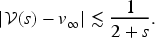
There exists such that, for all ,
In the following, we will write when there exists , independent of and depending on only through , such that . However, will usually depend on and the initial data.
Since is a solution to (RVM) with compactly supported data, it follows that
Hence the right hand sides of (1.4) and (1.5) are always bounded.
It is important to note that, according to Glassey and Schaeffer (1988, Theorem 1) and Glassey and Strauss (1987), for small compactly supported data or nearly neutral data, the unique associated classical solution to (RVM) satisfies Hypothesis 1.1. This proves that, when the data are compactly supported, Theorem 1.5 holds for small or nearly neutral data. Finally, our result applies to a subclass of the solutions constructed by Rein (1990) as well, those arising from compactly supported data.
We now state that for any verifying the above hypothesis, the distribution functions satisfy a modified scattering dynamic. Moreover, we are able to prove that the asymptotic limits are compactly supported.
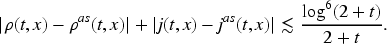
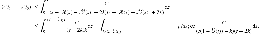
Let be a solution to (RVM) satisfying Hypothesis 1.1. Then, every verifies modified scattering. More precisely there exists and such that, for any and all verifying ,
Unlike Bigorgne (2025) and Pankavich and Ben-Artzi (2024) we modify the characteristics of the operator instead of . This is more consistent with the Lorentz invariance of (RVM) that we will exploit in a forthcoming article (Breton, In preparation) (see Remark 1.7). (To observe the Lorentz invariance of the Vlasov–Maxwell system, one has to write the Vlasov equation as in (RVM) rather than in (2.3) below). However, taking
In fact, these two formulations can be derived from each other and it will be more convenient to prove the latter one.
In a forthcoming article (Breton, In preparation), we will show that linear scattering, that is , is a non-generic phenomenon. More precisely, the initial data leading to linear scattering lie in a codimension 1 submanifold.
Ideas of the Proof
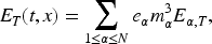
We detail here the arguments used to prove Theorem 1.5. Let be a solution to (RVM) that satisfies Hypothesis 1.1. For the sake of presentation, here we assume that so that . We begin by composing with the linear flow to consider . We then derive two key properties
Moreover, the spatial support of is included in , where . Consequently, the Lorentz force satisfies, on the support of ,
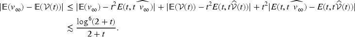
The first idea is to look for linear scattering, in which case we would have that converges as . For this matter, we compute
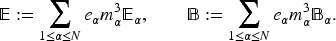
With our estimates, we can merely control the first term by , preventing us from concluding that converges as . Note that this is consistent with Remark 1.7. However, by further investigating the asymptotic behavior of , we can still expect to prove that converges along modifications of the linear characteristics. To achieve this, we are led to determine the leading order contribution of the source terms and in the Maxwell equations. For the linearized system, the asymptotic behavior of and is governed by the spatial average , which, in this setting, is a conserved quantity. To this end, we begin by proving the existence of the asymptotic charge such that converges to . Now, let . This allows us to consider the asymptotic charge and the asymptotic current densities
where is the inverse of . These densities satisfy
The previous arguments allow us to define , which verify
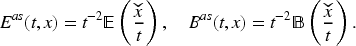
Although it is not immediately apparent in Sections 3.1–3.2, it turns out that and can be interpreted as follows. Let and be the solutions to
with trivial data at . Then for large enough, we have for all
Moreover, for large enough, we have in the Glassey–Strauss decomposition of the electromagnetic field , associated to the singular distribution function through Proposition 3.1. We refer to Bigorgne (2023b, Section 5) for more information.
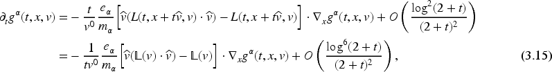
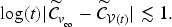
To conclude, it remains to prove the modified scattering statement for the density functions . Using the above estimates for the fields, we derive
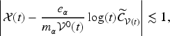
where . We finally introduce the correction
which, once multiplied by , measures how much the characteristics of the Vlasov operator deviate from the linear ones. It allows us to obtain the modified scattering statement and that the asymptotic state is compactly supported.
Structure of the Paper
Section 2 contains several statements that are needed in our proof of Theorem 1.5. We first introduce the function by composing with the linear flow. Then we compute the support of and two key properties on and its first order derivatives. We end this section by studying the asymptotic properties of and . Finally, in Section 3, we further investigate the asymptotic behavior of and show that the densities exhibit a modified scattering dynamic. Then, we prove the compactness of the support of (see Proposition 3.11), concluding the proof of Theorem 1.5.
Preliminary Results
In the following sections, we consider a solution to (RVM) that satisfies Hypothesis 1.1. We begin this section by giving a lemma about the inverse of .
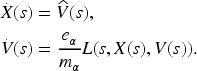
We define on the map by
In particular
Finally, the Jacobian determinant of is .
Let us begin by introducing, to simplify the notations,
Notice here that the support of is now included in with . Moreover, satisfies the following equation
From this we can introduce
Notice that this notation is consistent since . Moreover, the derivatives of can be expressed as the following
This means that for , will satisfy the following equation
Characteristics
We begin by introducing the characteristics of . Let be defined by the ODE
One can easily switch between the characteristics of and . In fact, taking , we derive the following ODE
Meaning that are the characteristics of starting from .
We will now show that the support of is bounded, uniformly in . From this we derive that the space support of is bounded by . Here, contrary to Glassey and Strauss (1987), we do not require smallness of the initial data to prove the result.
There exists a constant such that, for all and any
where . Moreover, if then
where . In particular, for in the support of , we have
The proof follows Wei and Yang (2021, Lemma 2.1). Let such that . This implies and thus we are working with . We begin by introducing
Using the ODE satisfied by , one finds
Here we used that is increasing. Now consider . Using (1.4) we derive,
Computing the last two integrals we derive
where
From this we follow Wei and Yang (2021, Lemma 2.1) and find a constant independent of such that
Hence, there exists such that, for ,
It remains to prove the estimate on the support of . Since and is constant along its characteristics, we know that . So we derive directly
Implying directly . This gives the inclusion for the support of as well as the other two inequalities.
One can easily go back to to find its support. In fact, we have
Moreover, since is a solution to (RVM) with compactly supported initial data,
Properties of
With these properties for the characteristics of in mind, we now want to estimate the support of and control its derivatives.
There exists a constant such that, for all and any ,
With the previous notations, we have, thanks to (1.4),
Now, thanks to Proposition 2.3, we have , which implies
We now estimate and its first order derivatives.
Consider with . We have the following estimates, for any ,
The first estimate is immediate by using the characteristics. Then, recall (2.6) and let be the associated operator such that . We have
Now let us consider the characteristics of . Recall Lemma 2.3, so for , we have
This implies the following estimates
We can now use the equation satisfied by and to derive, thanks to Duhamel’s principle,
where in the integral are evaluated at . Since is integrable, by Grönwall’s inequality we have for all
We now apply Gronwall’s inequality to . Since is integrable we derive
and the estimate on follows. Inserting the estimate on in (2.13) we derive the other estimate. Finally, taking , we derive the result.
From (2.4)–(2.5) and the above proposition, one can easily derive estimates on the derivatives of . Moreover, the derivatives of (resp. ) satisfy the same estimates as those satisfied by (resp. ).
Convergence of the Spatial Average
We focus on the spatial average of since this quantity governs the asymptotic behavior of the source terms in the Maxwell equations.
The second term of the right-hand side can directly be dealt with. Indeed, thanks to (1.4), Lemma 2.3 and Propositions 2.5–2.6, we have
It remains to study the first term. By integration by parts, we derive
Again from (1.5), Lemma 2.3 and Propositions 2.5–2.6, we obtain
Finally, combining these two estimates, we obtain
Now, since is integrable in , this proves the existence of the limit . Moreover has its support in so we already know that .
Finally, since is continuous and converges uniformly towards we know that is also continuous.
Link Between the Particle Density and the Asymptotic Charge
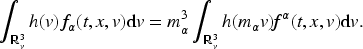
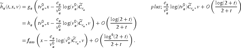
In Glassey and Strauss (1987) they prove that the velocity average decays like . Here we provide the asymptotic expansion of . The following proposition justifies, for and , the asymptotic expansion of the charge and current densities stated in the outline of the proof. Recall, in particular, that .
Let . Then for any , all and all we have
Since and are continuous and compactly supported, it is enough to prove the estimate for . We begin by the change of variable so that
Applying Proposition 2.8 to , in view of the support of and , we derive
This leaves us with proving that, for any ,
First, use Lemma 2.1 and the change of variables to derive
Here we observe the correct function evaluated in instead of . We force the desired term to appear by writing
We now show that and are both .
Estimate of . For a fixed we want to apply the mean value theorem to . Since , by differentiating we get
by Proposition 2.6. Now by the mean value theorem and using the support of , we get,
Estimate of . Recall that , this allows us to get, for and ,
implying that
Combining these estimates, we get (2.18). With (2.17), this implies the result.
Modified Scattering
Estimations of the Fields
Let us start by recalling the Glassey–Strauss decomposition.
Let and . The following decomposition of the field holds.
where
with
and .
The same decomposition holds for . The expression of and is obtained by replacing by in and . Moreover, the expression of only depends on the initial data, so the estimates follow similarly in the next propositions. In the following, we restrict ourselves to the study of as the analysis of is similar.
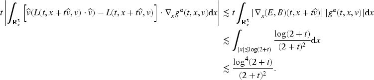
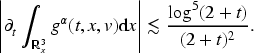
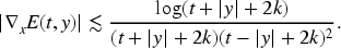
As stated in the introduction, we want to identify the part of that decays like for , with . We start by showing that and decay at least as . For this, we have to improve the estimate obtained by Glassey and Strauss (1987) for .
For all , we have the following estimate
First, recall the expression of from (3.4). Using the support of every term of is bounded by
which implies the result.
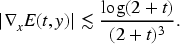
For all , we have the following estimate
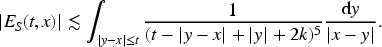
Here we slightly refine the analysis performed for in Glassey and Strauss (1987, Lemma 6) by exploiting the support of . First recall (3.3) and . By integration by parts we obtain
Now, recall that the kernel where appears is bounded on the support of . Then by Proposition 2.9 we have
where and . Moreover, the bounds of the integral are and . We first write, as and ,
If , then . Otherwise, and we can split in two parts
Asymptotic Expansion of the Fields
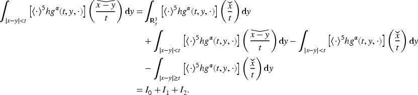
Having proved the estimate on , it remains to study . The goal of this subsection is to find a form of asymptotic expansion for .
Let . Consider
with and . Then, .
Using the support of we know that we integrate over so and thus , implying that the integral is well defined. The continuity follows as .
We begin by performing the change of variables , so that
where
Let . Then, there exists such that for all and all
where is a constant depending on .
We begin by showing that for large enough (depending on ) and we have
Write . On the support of we know that . Thus, for , we have . Now, on the support of again we have
leaving us with . Finally, for
we derive and thus .
Consider now
so that
Recall (3.10). Using the support of and , vanishes for . Thus, for we have, on the support of ,
We now apply Proposition 2.9 with . Since we derive
which concludes the proof.
Before giving the final estimate, we define the asymptotic fields and by
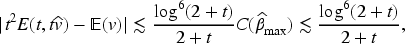
Let and . We have the following estimate
where is a constant depending only on and .
This follows from the decomposition and Propositions 3.3–3.4 and 3.6.
Proof of the Modified Scattering Theorem
In this subsection, we finish the proof of Theorem 1.5. First, let us detail two preliminary results.
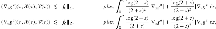
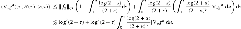
For any , all and all in the support of , i.e. , we have
Using Corollary 3.7 we already know that for , since
where here we omit the constant since it only depends on and . Now we only need to prove that
We will prove the above inequality using the mean value theorem. For this we need to consider with , so that . Using (1.5) we obtain
Consider large enough so we have . This implies and then as well as . This grants us
Now, the mean value theorem and allow us to derive (3.14) and obtain the result for . It also holds on the compact interval of time since and are bounded.
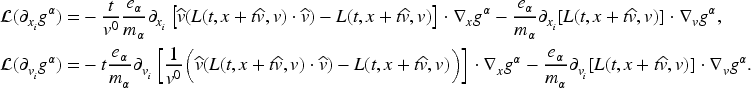
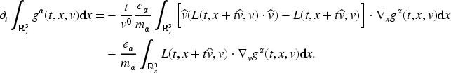
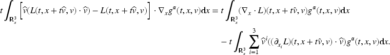
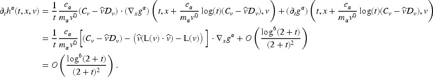
Now, recall (2.6). Thanks to the estimate (1.4) and Propositions 2.6 and 3.8, we have
where is the asymptotic Lorentz force. We observe that the first term on the right-hand side is of order , which is not integrable. We thus consider corrections to the linear characteristics to cancel it. We define the following corrections
Now, let us consider
For any , all and all , we have
We directly have, thanks to the above equation (3.15) on ,
Consequently, there exists such that
This directly implies the result, with , where we recall and .
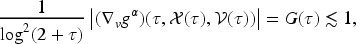
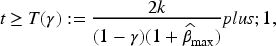
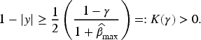
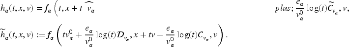
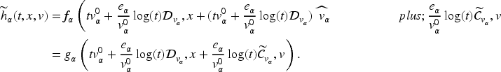
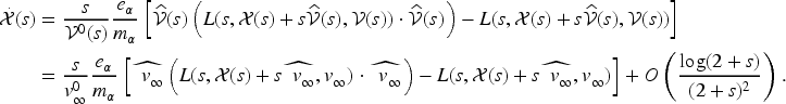
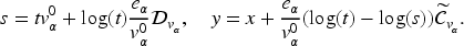
It remains to prove the estimate of Theorem 1.5. For this, write and let
Notice that for to be well-defined, one needs to have . Since , this holds whenever is large enough.
We already know that
Moreover,
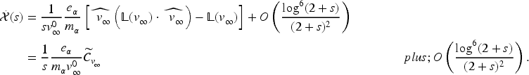
Now we know that, thanks to (1.4) and Proposition 2.6, . Hence, by the mean value theorem, we derive, for large enough,
Finally, using the expression of , we obtain
So we derive the estimate of Theorem 1.5 by taking . However, to prove Theorem 1.5, it remains to show that has a compact support.
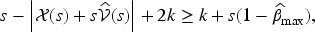
There exists and a constant such that, for all
i.e. is compactly supported, uniformly in .
Recall the expression of
and assume . Consider the characteristics
Now recall the ODE (2.7) satisfied by . We have , according to Lemma 2.3 and (1.4). Thus, there exists such that
Now, using (1.4)–(1.5), the mean value theorem and the above equation, we derive
This grants us, by applying Proposition 3.8,
By integrating we derive, for ,
Finally, one can notice that since and , we have . Then, it yields
By deriving the same estimate for , we obtain for large enough
So finally,
that is, since and we have
The functions and are compactly supported. That is , such that ,
Since , the first result is immediate. Now, notice that with
Assume , then, by Proposition 3.11, and . Moreover,
so is bounded, uniformly in on the support of , by . Then .
The functions and are all compactly supported.
Footnotes
Funding
The author received no financial support for the research, authorship and/or publication of this article.
Declaration of Conflicting Interests
The author declared no potential conflicts of interest with respect to the research, authorship, and/or publication of this article.
ORCID iD
Emile Breton
References
1.
BigorgneL. (2020). Sharp asymptotic behavior of solutions of the 3D Vlasov–Maxwell system with small data. Communications in Mathematical Physics, 376(2), 893–992.
2.
BigorgneL. (2023b). Scattering map for the Vlasov–Maxwell system around source-free electromagnetic fields. arXiv: 2312.12214.
3.
BigorgneL. (2025). Global existence and modified scattering for the solutions to the Vlasov-Maxwell system with a small distribution function. Analysis & PDE, 18(3), 629–714.
4.
BigorgneL.RuizR. V. (2024). Late-time asymptotics of small data solutions for the Vlasov–Poisson system. arXiv: 2404.05812 [math.AP].
5.
BigorgneL.Velozo RuizA.Velozo RuizR. (2025). Modified scattering of small data solutions for the Vlasov–Poisson system with a repulsive potential. SIAM Journal on Mathematical Analysis, 57(1), 714–752.
6.
BretonE. (2025). A note on the non -asymptotic completeness of the Vlasov–Maxwell system. arXiv: 2509.04025.
7.
ChoiS. H.HaS. Y. (2011). Asymptotic behavior of the nonlinear vlasov equation with a self-consistent force. SIAM Journal on Mathematical Analysis, 43(5), 2050–2077.
8.
ChoiS. H.KwonS. (2016). Modified scattering for the Vlasov–Poisson system. Nonlinearity, 29(9), 2755.
9.
FlynnP.OuyangZ.PausaderB.WidmayerK. (2023). Scattering map for the Vlasov–Poisson system. Peking Mathematical Journal, 6(2), 365–392.
10.
GlasseyR. T.SchaefferJ. W. (1988). Global existence for the relativistic Vlasov–Maxwell system with nearly neutral initial data. Communications in Mathematical Physics, 119(3), 353–384.
11.
GlasseyR. T.StraussW. A. (1987). Absence of shocks in an initially dilute collisionless plasma. Communications in Mathematical Physics, 113(2), 191–208.
12.
IonescuA. D.PausaderB.WangX.WidmayerK. (2021). On the asymptotic behavior of solutions to the Vlasov–Poisson system. International Mathematics Research Notices, 2022(12), 8865–8889.
13.
LukJ.StrainR. M. (2016). Strichartz estimates and moment bounds for the relativistic Vlasov–Maxwell system. Archive for Rational Mechanics and Analysis, 219(1), 445–552.
14.
PankavichS. (2022). Asymptotic dynamics of dispersive, collisionless plasmas. Communications in Mathematical Physics, 391(2), 455–493.
15.
PankavichS.Ben-ArtziJ. (2024). Modified scattering of solutions to the relativistic Vlasov–Maxwell system inside the light cone. arXiv: 2306.11725 [math.AP].
16.
PausaderB.WidmayerK. (2021). Stability of a point charge for the Vlasov–Poisson system: The radial case. Communications in Mathematical Physics, 385(3), 1741–1769.
17.
PausaderB.WidmayerK.YangJ. (2024). Stability of a point charge for the repulsive Vlasov–Poisson system. Journal of the European Mathematical Society, Published online first.
18.
ReinG. (1990). Generic global solutions of the relativistic Vlasov–Maxwell system of plasma physics. Communications in Mathematical Physics, 135(1), 41–78.
19.
SchaefferJ. (2004). A small data theorem for collisionless plasma that includes high velocity particles. Indiana University Mathematics Journal, 53(1), 1–34.
20.
SchlueV.TaylorM. (2024). Inverse modified scattering and polyhomogeneous expansions for the Vlasov–Poisson system. arXiv: 2404.15885 [math.AP].
21.
WangX. (2022). Propagation of regularity and long time behavior of the 3D massive relativistic transport equation II: Vlasov–Maxwell system. Communications in Mathematical Physics, 389(2), 715–812.
22.
WeiD.YangS. (2021). On the 3D relativistic Vlasov–Maxwell system with large Maxwell field. Communications in Mathematical Physics, 383(3), 2275–2307.