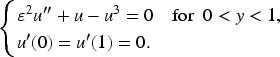
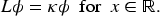
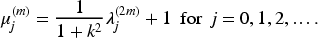
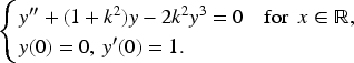
The Lamé Equation on a Circle and Applications to Singular Limit Eigenvalue Problems

Abstract

Let $n \in {1, 2, \dots}$ , $ℓ \in {1, 2}$ and $0 < k < 1$ . We are concerned with the eigenvalues of the Lamé equation of the form $\begin{aligned} - ϕ^{″} + ℓ (ℓ + 1) {e_{3} + k^{2} {sn}^{2} (x, k)} ϕ = λ ϕ for x \in R / 2 n K (k) Z, \end{aligned}$ where $e_{3} := - (1 + k^{2}) / 3$ is a constant, $sn (x, k)$ denotes Jacobi’s elliptic function and $K (k)$ denotes the complete elliptic integral of the first kind. Using integral representations of two independent solutions, we obtain exact expressions of all eigenvalues and establish asymptotic formulas for all eigenvalues as $k \to 1$ . It is known that the Lamé equation appears as a linearized eigenvalue problem of important semilinear elliptic equations including the Allen–Cahn equation, a scalar field equation and the sine-Poisson equation. We also establish asymptotic formulas for the eigenvalues of the linearization of various boundary value problems of semilinear elliptic equations.

Keywords

asymptotic formula for the eigenvalue singularly perturbed elliptic problems linearized eigenvalue problems Jacobi’s elliptic functions complete elliptic integrals

1. Introduction and Main Theorems

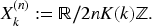
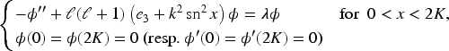
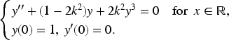
Let $n \geq 1$ and $ℓ \geq 1$ be positive integers and let $0 < k < 1$ . We are concerned with the Lamé equation of the form

\begin{aligned} - ϕ^{″} + ℓ (ℓ + 1) {e_{3} + k^{2} {sn}^{2} (x, k)} ϕ = λ ϕ for x \in X_{k}^{(n)}, \end{aligned}

(1.1)

where

e_{3} := - (1 + k^{2}) / 3

is a constant,

sn (x, k)

denotes Jacobi’s elliptic function,

K (k)

denotes the complete elliptic integral of the first kind and the domain is a circle

\begin{aligned} X_{k}^{(n)} := R / 2 n K (k) Z . \end{aligned}

In this paper we frequently use the complete elliptic integral of the first kind

K (k)

, the Jacobi elliptic functions

sn (x, k)

cn (x, k)

and

dn (x, k)

and the Weierstrass elliptic function

℘ (z)

. Definitions and basic properties of elliptic functions and elliptic integrals are summarized in Section 7 of the present paper. Hereafter,

sn x

cn x

and

dn x

stand for

sn (x, k)

cn (x, k)

and

dn (x, k)

, respectively.

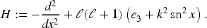
The Lamé equation appears in various contexts of mathematical sciences. One of the main concerns for the Lamé equation is spectra of the corresponding operator

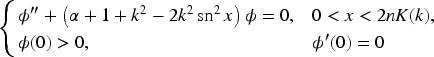
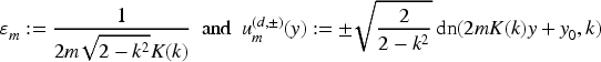
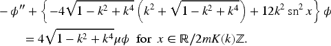
\begin{aligned} H := - \frac{d^{2}}{d x^{2}} + ℓ (ℓ + 1) (e_{3} + k^{2} {sn}^{2} x) . \end{aligned}

The eigenvalue problem (1.1) is classical. However, detailed descriptions of the eigenvalues of (1.1) seem to be unknown, because various integral formulas related to complete elliptic integrals given in Subsection 7.4 are needed and they were found recently. The first aim of the present paper is to obtain asymptotic formulas for all eigenvalues of

H

L^{2} (X_{k}^{(n)})

k \to 1

in the case

ℓ = 1, 2

. When

ℓ = 1

, the following expression of (1.1) is useful:

\begin{aligned} - ϕ^{″} + (- 1 - k^{2} + 2 k^{2} {sn}^{2} x) ϕ = α ϕ for x \in X_{k}^{(n)}, \end{aligned}

(1.2)

where

α := λ - (ℓ^{2} + ℓ - 3) e_{3}

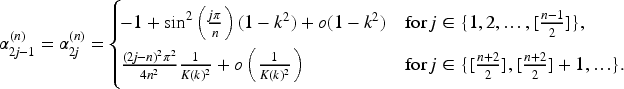
is a new spectral parameter for (1.2). The first main result is the following:

Theorem 1.1

ℓ = 1

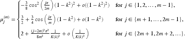
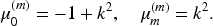
Let $n \geq 1$ . Let ${α_{j}^{(n)}}_{j = 0}^{\infty}$ , $α_{0}^{(n)} < α_{1}^{(n)} \leq α_{2}^{(n)} \leq \dots$ , be the eigenvalues of (1.2). Then the following hold:

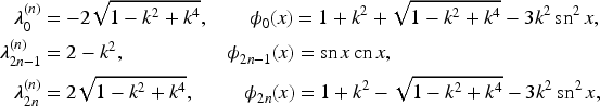
(i) The first eigenpair is given by

\begin{aligned} α_{0}^{(n)} = - 1, ϕ_{0} (x) = dn x, \end{aligned}

and

α_{0}^{(n)}

is simple. If

n

is even, then the following two pairs are eigenpairs:

\begin{aligned} α_{n - 1}^{(n)} & = - k^{2}, ϕ_{n - 1} (x) = cn x, \\ α_{n}^{(n)} & = 0, ϕ_{n} (x) = sn x, \end{aligned}

and the two eigenvalues

α_{n - 1}^{(n)}

and

α_{n}^{(n)}

are simple.

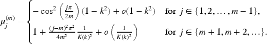
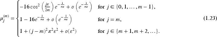
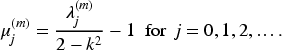
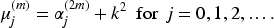
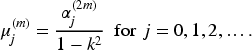
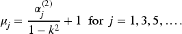
(ii) The other eigenvalues have multiplicity $2$ . Moreover, as $k \to 1$ ,

\begin{aligned} α_{2 j - 1}^{(n)} = α_{2 j}^{(n)} = {\begin{cases} - 1 + \sin^{2} (\frac{j π}{n}) (1 - k^{2}) + o (1 - k^{2}) & for j \in {1, 2, \dots, [\frac{n - 1}{2}]}, \\ \frac{(2 j - n)^{2} π^{2}}{4 n^{2}} \frac{1}{K {(k)}^{2}} + o (\frac{1}{K {(k)}^{2}}) & for j \in {[\frac{n + 2}{2}], [\frac{n + 2}{2}] + 1, \dots} . \end{cases} \end{aligned}

Although the three eigenvalues $α_{0}^{(n)}$ , $α_{n - 1}^{(n)}$ and $α_{n}^{(n)}$ given in Theorem 1.1 (i) and associated eigenfunctions, which are called the Lamé functions, are well known, we include them to cover all the eigenvalues.

Remark 1.2
(i) If $n$ is odd, then $α_{0}^{(n)}$ is simple and the other eigenvalues have multiplicity $2$ , i.e., $α_{1}^{(n)} = α_{2}^{(n)} < α_{3}^{(n)} = α_{4}^{(n)} < α_{5}^{(n)} = α_{6}^{(n)} < \dots$ . Note that neither $- k^{2}$ nor $0$ is an eigenvalue. If $n$ is even, then $α_{0}^{(n)}$ , $α_{n - 1}^{(n)}$ and $α_{n}^{(n)}$ are simple and the other eigenvalues have multiplicity $2$ .

(ii) The spectral set of (1.2) on $L^{2} (R)$ is
$\begin{aligned} [- 1, - k^{2}] \cup [0, \infty) . \end{aligned}$
(1.3)
All eigenvalues in Theorem 1.1 are on this set.

(iii) As $k \to 1$ , the first $n$ eigenvalues are on the first spectral band of (1.3) and they converge to $- 1$ . The other eigenvalues are on the second spectral band of (1.3) and they converge to $0$ .

When $ℓ = 2$ , (1.1) becomes the following:
$\begin{aligned} - ϕ^{″} + (- 2 - 2 k^{2} + 6 k^{2} {sn}^{2} x) ϕ = λ ϕ for x \in X_{k}^{(n)} . \end{aligned}$
(1.4)
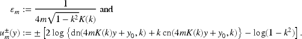
In this case we do not change the spectral parameter $λ$ . The second main result is the following:
Theorem 1.3 $ℓ = 2$

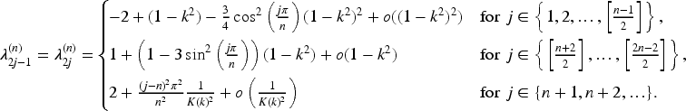
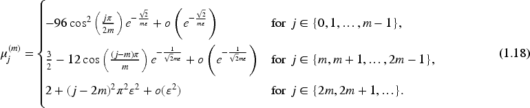
Let $n \geq 1$ . Let ${λ_{j}^{(n)}}_{j = 0}^{\infty}$ , $λ_{0}^{(n)} < λ_{1}^{(n)} \leq λ_{2}^{(n)} \leq \dots$ , be the eigenvalues of (1.4). Then the following hold:

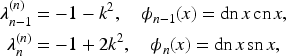
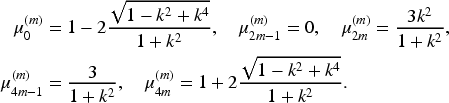
(i) The following three pairs are eigenpairs:

\begin{aligned} λ_{0}^{(n)} & = - 2 \sqrt{1 - k^{2} + k^{4}}, ϕ_{0} (x) = 1 + k^{2} + \sqrt{1 - k^{2} + k^{4}} - 3 k^{2} {sn}^{2} x, \\ λ_{2 n - 1}^{(n)} & = 2 - k^{2}, ϕ_{2 n - 1} (x) = sn x cn x, \\ λ_{2 n}^{(n)} & = 2 \sqrt{1 - k^{2} + k^{4}}, ϕ_{2 n} (x) = 1 + k^{2} - \sqrt{1 - k^{2} + k^{4}} - 3 k^{2} {sn}^{2} x, \end{aligned}

and three eigenvalues

λ_{0}^{(n)}

λ_{2 n - 1}^{(n)}

and

λ_{2 n}^{(n)}

are simple. If

n

is even, then the following two pairs are also eigenpairs:

\begin{aligned} λ_{n - 1}^{(n)} & = - 1 - k^{2}, ϕ_{n - 1} (x) = dn x cn x, \\ λ_{n}^{(n)} & = - 1 + 2 k^{2}, ϕ_{n} (x) = dn x sn x, \end{aligned}

and two eigenvalues

λ_{n - 1}^{(n)}

and

λ_{n}^{(n)}

are simple.

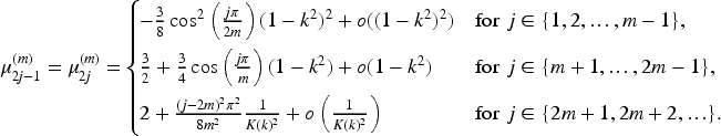
(ii) The other eigenvalues have multiplicity $2$ . Moreover, as $k \to 1$ ,

\begin{aligned} λ_{2 j - 1}^{(n)} = λ_{2 j}^{(n)} = {\begin{cases} - 2 + (1 - k^{2}) - \frac{3}{4} \cos^{2} (\frac{j π}{n}) (1 - k^{2})^{2} + o ((1 - k^{2})^{2}) & for j \in {1, 2, \dots, [\frac{n - 1}{2}]}, \\ 1 + (1 - 3 \sin^{2} (\frac{j π}{n})) (1 - k^{2}) + o (1 - k^{2}) & for j \in {[\frac{n + 2}{2}], \dots, [\frac{2 n - 2}{2}]}, \\ 2 + \frac{(j - n)^{2} π^{2}}{n^{2}} \frac{1}{K {(k)}^{2}} + o (\frac{1}{K {(k)}^{2}}) & for j \in {n + 1, n + 2, \dots} . \end{cases} \end{aligned}

Although the five eigenvalues given in Theorem 1.3 (i) and corresponding eigenfunctions are well known, we include them to cover all the eigenvalues.

Remark 1.4
(i) If $n$ is odd, then $λ_{0}^{(n)}$ , $λ_{2 n - 1}^{(n)}$ and $λ_{2 n}^{(n)}$ are simple and the other eigenvalues have a multiplicity $2$ . Note that neither $- 1 - k^{2}$ nor $- 1 + 2 k^{2}$ is an eigenvalue. If $n$ is even, then $λ_{0}^{(n)}$ , $λ_{n - 1}^{(n)}$ , $λ_{n}^{(n)}$ , $λ_{2 n - 1}^{(n)}$ and $λ_{2 n}^{(n)}$ are simple and other eigenvalues have a multiplicity $2$ .

(ii) The spectral set of (1.4) on $L^{2} (R)$ is
$\begin{aligned} [- 2 \sqrt{1 - k^{2} + k^{4}}, - 1 - k^{2}] \cup [- 1 + 2 k^{2}, 2 - k^{2}] \cup [2 \sqrt{1 - k^{2} + k^{4}}, \infty) . \end{aligned}$
(1.5)
All eigenvalues in Theorem 1.3 are on this set.

(iii) It follows from Theorem 1.3 that the first $n$ eigenvalues are on the first spectral band of (1.5) and they converge to $- 2$ ( $k \to 1$ ). The second $n$ eigenvalues are on the second spectral band and they converge to $1$ . The other eigenvalues are on the third spectral band and they converge to $2$ .

The second aim of the present paper is applications of Theorems 1.1 and 1.3 to singularly perturbed nonlinear elliptic problems. It was found in Liang et al. (1992) that the Lamé equation appears as linearized eigenvalue problems of important semilinear elliptic equations, namely
the Allen–Cahn equation $ε^{2} u^{″} + u - u^{3} = 0$ , ( $ℓ = 2$ ),

the scalar field equation $ε^{2} u^{″} - u + u^{3} = 0$ , ( $ℓ = 2$ ),

the sine-Poisson equation $ε^{2} u^{″} + \sin u = 0$ , ( $ℓ = 1$ ).
However, only special eigenvalues, which are given by Theorems 1.1 (i) and 1.3 (i), were studied in Liang et al. (1992).

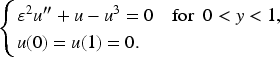
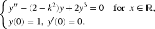
Let us explain some details of our results here. For example, we consider the Allen–Cahn equation on $[0, 1)$ with periodic boundary condition:
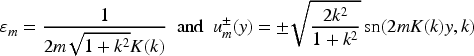
$\begin{aligned} ε^{2} u^{″} + u - u^{3} = 0 for y \in R / Z, \end{aligned}$
(1.6)
where $u (y)$ is an unknown function. All nontrivial solutions of (1.6) can be written as
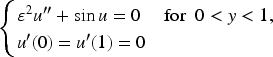
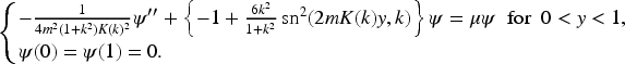
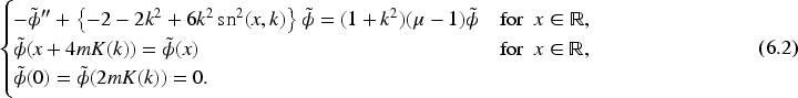
$\begin{aligned} ε := \frac{1}{4 m \sqrt{1 + k^{2}} K (k)} and u_{m}^{\pm} (y) := \pm \sqrt{\frac{2 k^{2}}{1 + k^{2}}} sn (4 m K (k) y + y_{0}) \end{aligned}$
(1.7)
for $m = 1, 2, \dots$ and $0 < k < 1$ . We consider the case $y_{0} = 0$ . The linearized eigenvalue problem becomes
$\begin{aligned} ε^{2} ψ^{″} + {1 - 3 (u_{m}^{\pm} (y))^{2}} ψ = - μ ψ for y \in R / Z, \end{aligned}$
(1.8)
where $ψ (y)$ is an unknown function. Let $x := 4 m K (k) y$ and $ϕ (x) := ψ (y)$ . Then, (1.8) is equivalent to
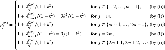
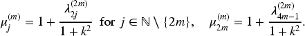
$\begin{aligned} - ϕ^{″} + (- 2 - 2 k^{2} + 6 k^{2} {sn}^{2} x) ϕ = (1 + k^{2}) (μ - 1) ϕ for x \in R / 4 m K (k) Z . \end{aligned}$
(1.9)
Note that $ℓ = 2$ because $ℓ (ℓ + 1) = 6$ . Let $n = 2 m$ . Then, (1.9) is equivalent to (1.4) with $(1 + k^{2}) (μ - 1) = λ$ . Therefore, each eigenvalue $μ_{j}^{(m)}$ , $j \geq 0$ , of (1.9) is given by
$\begin{aligned} μ_{j}^{(m)} = \frac{λ_{j}^{(2 m)}}{1 + k^{2}} + 1 for j = 0, 1, 2, \dots . \end{aligned}$
(1.10)
Now, we can obtain asymptotic formulas of the eigenvalues of (1.8), using Theorem 1.3 and (1.10).
Corollary 1.5
Let $m \geq 1$ . Let ${μ_{j}^{(m)}}_{j = 0}^{\infty}$ denote the eigenvalues of (1.8). Then the following hold:

(i) The eigenvalues $μ_{0}^{(m)}$ , $μ_{2 m - 1}^{(m)}$ , $μ_{2 m}^{(m)}$ , $μ_{4 m - 1}^{(m)}$ and $μ_{4 m}^{(m)}$ are simple and they are given by
$\begin{aligned} μ_{0}^{(m)} & = 1 - 2 \frac{\sqrt{1 - k^{2} + k^{4}}}{1 + k^{2}}, μ_{2 m - 1}^{(m)} = 0, μ_{2 m}^{(m)} = \frac{3 k^{2}}{1 + k^{2}}, \\ μ_{4 m - 1}^{(m)} & = \frac{3}{1 + k^{2}}, μ_{4 m}^{(m)} = 1 + 2 \frac{\sqrt{1 - k^{2} + k^{4}}}{1 + k^{2}} . \end{aligned}$
(ii) The other eigenvalues have multiplicity $2$ . Moreover, as $k \to 1$ ,
$\begin{aligned} μ_{2 j - 1}^{(m)} = μ_{2 j}^{(m)} = {\begin{cases} - \frac{3}{8} \cos^{2} (\frac{j π}{2 m}) (1 - k^{2})^{2} + o ((1 - k^{2})^{2}) & for j \in {1, 2, \dots, m - 1}, \\ \frac{3}{2} + \frac{3}{4} \cos (\frac{j π}{m}) (1 - k^{2}) + o (1 - k^{2}) & for j \in {m + 1, \dots, 2 m - 1}, \\ 2 + \frac{(j - 2 m)^{2} π^{2}}{8 m^{2}} \frac{1}{K {(k)}^{2}} + o (\frac{1}{K {(k)}^{2}}) & for j \in {2 m + 1, 2 m + 2, \dots} . \end{cases} \end{aligned}$

We consider the limit $k \to 1$ . Since $\sqrt{1 + k^{2}} K (k)$ is increasing in $k$ and $\sqrt{1 + k^{2}} K (k) \to \infty$ , by (1.7) we see that $k \to 1$ is equivalent to $ε \to 0$ . Hence, (1.8) is the so-called singular limit eigenvalue problem. A singular limit of a solution as $ε \to 0$ appears in many branches of mathematical sciences, and the asymptotic formula of the eigenvalue $μ_{j}^{(m)}$ as $ε \to 0$ has attracted a great attention. For example, the asymptotic formula of the eigenvalue as $ε \to 0$ plays a crucial role in a limit of energy of various models in quantum physics (Funakubo et al., 1990; Liang et al., 1992; Manton & Samols, 1988; Smondyrev et al., 1995), in very slow dynamics in coarsening phenomena of the Allen–Cahn (real Ginzburg–Landau) equation (Carr & Pego, 1989; Eckmann & Rougemont, 1998) and in a metastability of spiky stationary patterns of the shadow Gierer–Meinhardt system in morphogenesis (de Groen & Karadzhov, 2002; Iron & Ward, 2000). By Lemma 7.1 we have
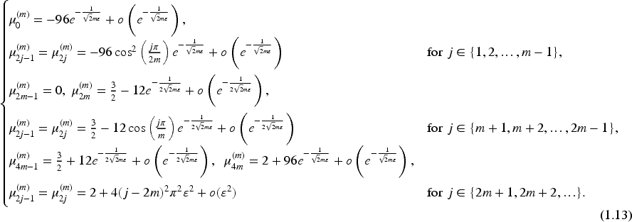
$\begin{aligned} \sqrt{1 - k^{2}} K (k) \to 0 as k \to 1. \end{aligned}$
(1.11)
Using (1.7), (1.11) and Lemma 7.1, we obtain the following: As $ε \to 0$ ,
$\begin{aligned} \frac{1}{K (k)} = 4 \sqrt{2} m ε (1 + o (1)) and 1 - k^{2} = e^{- \frac{1}{2 \sqrt{2} m ε}} (1 + o (1)) . \end{aligned}$
(1.12)
By (1.12) and Corollary 1.5 we can obtain the following asymptotic formulas: As $ε \to 0$ ,
$\begin{aligned} {\begin{cases} μ_{0}^{(m)} = - 96 e^{- \frac{1}{\sqrt{2} m ε}} + o (e^{- \frac{1}{\sqrt{2} m ε}}), \\ μ_{2 j - 1}^{(m)} = μ_{2 j}^{(m)} = - 96 \cos^{2} (\frac{j π}{2 m}) e^{- \frac{1}{\sqrt{2} m ε}} + o (e^{- \frac{1}{\sqrt{2} m ε}}) & for j \in {1, 2, \dots, m - 1}, \\ μ_{2 m - 1}^{(m)} = 0, μ_{2 m}^{(m)} = \frac{3}{2} - 12 e^{- \frac{1}{2 \sqrt{2} m ε}} + o (e^{- \frac{1}{2 \sqrt{2} m ε}}), \\ μ_{2 j - 1}^{(m)} = μ_{2 j}^{(m)} = \frac{3}{2} - 12 \cos (\frac{j π}{m}) e^{- \frac{1}{2 \sqrt{2} m ε}} + o (e^{- \frac{1}{2 \sqrt{2} m ε}}) & for j \in {m + 1, m + 2, \dots, 2 m - 1}, \\ μ_{4 m - 1}^{(m)} = \frac{3}{2} + 12 e^{- \frac{1}{2 \sqrt{2} m ε}} + o (e^{- \frac{1}{2 \sqrt{2} m ε}}), μ_{4 m}^{(m)} = 2 + 96 e^{- \frac{1}{\sqrt{2} m ε}} + o (e^{- \frac{1}{\sqrt{2} m ε}}), \\ μ_{2 j - 1}^{(m)} = μ_{2 j}^{(m)} = 2 + 4 (j - 2 m)^{2} π^{2} ε^{2} + o (ε^{2}) & for j \in {2 m + 1, 2 m + 2, \dots} . \end{cases} \end{aligned}$
(1.13)
In summary the eigenvalue relation (1.10) is crucial to obtain (1.13).

We show that the eigenvalues for both Dirichlet and Neumann problems can be expressed by using eigenvalues for periodic problems. For example, we consider the Neumann problem
$\begin{aligned} {\begin{cases} ε^{2} u^{″} + u - u^{3} = 0 & for 0 < y < 1, \\ u^{'} (0) = u^{'} (1) = 0. \end{cases} \end{aligned}$
All nontrivial solutions can be expressed as
$\begin{aligned} ε := \frac{1}{2 m \sqrt{1 + k^{2}} K (k)} and u_{m}^{\pm} (y) := \pm \sqrt{\frac{2 k^{2}}{1 + k^{2}}} sn ((2 m y + 1) K (k)) \end{aligned}$
(1.14)
for $m = 1, 2, \dots$ and $0 < k < 1$ . The first three eigenvalues $μ_{j}^{(1)}$ , $j \in {0, 1, 2}$ , for $1$ -mode solutions $u_{1}^{\pm} (y)$ were obtained in Wakasa (2006). We will see in (2) of Subsection 6.1 that the three eigenvalues correspond to $λ_{0}$ , $λ_{n}$ and $λ_{2 n}$ in Theorem 1.3 (i). In Wakasa and Yotsutani (2015) exact expressions of the other eigenvalues were obtained and asymptotic formulas were established. Now, we show that the same asymptotic formula as in Wakasa and Yotsutani (2015) can be obtained by Theorem 1.3. Let ${μ_{j}^{(m)}}_{j = 0}^{\infty}$ denote the eigenvalues of the associated eigenvalue problem
$\begin{aligned} {\begin{cases} ε^{2} ψ^{″} + {1 - 3 (u_{m}^{\pm} (y))^{2}} ψ = - μ ψ & for 0 < y < 1, \\ ψ^{'} (0) = ψ^{'} (1) = 0. \end{cases} \end{aligned}$
(1.15)
In Subsection 6.1 we prove the following eigenvalue relation
$\begin{aligned} μ_{j}^{(m)} = \frac{λ_{2 j}^{(2 m)}}{1 + k^{2}} + 1 for j = 0, 1, 2, \dots . \end{aligned}$
(1.16)
Using (1.16) and Theorem 1.3, we obtain the following:
Corollary 1.6
Let ${μ_{j}^{(m)}}_{j = 0}^{\infty}$ denote the eigenvalues of (1.15). Then, every eigenvalue is simple and the following hold:

(i) Three eigenvalues $μ_{0}^{(m)}$ , $μ_{m}^{(m)}$ and $μ_{2 m}^{(m)}$ are given by
$\begin{aligned} μ_{0}^{(m)} = 1 - 2 \frac{\sqrt{1 - k^{2} + k^{4}}}{1 + k^{2}}, μ_{m}^{(m)} = \frac{3 k^{2}}{1 + k^{2}}, μ_{2 m}^{(m)} = 1 + 2 \frac{\sqrt{1 - k^{2} + k^{4}}}{1 + k^{2}} . \end{aligned}$
(ii) The other eigenvalues satisfy the following: As $k \to 1$ ,
$\begin{aligned} μ_{j}^{(m)} = {\begin{cases} - \frac{3}{8} \cos^{2} (\frac{j π}{2 m}) (1 - k^{2})^{2} + o ((1 - k^{2})^{2}) & for j \in {1, 2, \dots, m - 1}, \\ \frac{3}{2} + \frac{3}{4} \cos (\frac{j π}{m}) (1 - k^{2}) + o (1 - k^{2}) & for j \in {m + 1, \dots, 2 m - 1}, \\ 2 + \frac{(j - 2 m)^{2} π^{2}}{8 m^{2}} \frac{1}{K {(k)}^{2}} + o (\frac{1}{K {(k)}^{2}}) & for j \in {2 m + 1, 2 m + 2, \dots} . \end{cases} \end{aligned}$

Note that neither $λ_{2 m - 1}^{(2 m)}$ nor $λ_{4 m - 1}^{(2 m)}$ is used in the Neumann problem. By (1.11), (1.14) and Lemma 7.1 we obtain the following: As $ε \to 0$ ,
$\begin{aligned} \frac{1}{K (k)} = 2 \sqrt{2} m ε (1 + o (1)) and 1 - k^{2} = 16 e^{- \frac{1}{\sqrt{2} n ε}} (1 + o (1)) . \end{aligned}$
(1.17)
By (1.17) and Corollary 1.6 we obtain the following asymptotic formulas: As $ε \to 0$ ,
$\begin{aligned} μ_{j}^{(m)} = {\begin{cases} - 96 \cos^{2} (\frac{j π}{2 m}) e^{- \frac{\sqrt{2}}{m ε}} + o (e^{- \frac{\sqrt{2}}{m ε}}) & for j \in {0, 1, \dots, m - 1}, \\ \frac{3}{2} - 12 \cos (\frac{(j - m) π}{m}) e^{- \frac{1}{\sqrt{2} m ε}} + o (e^{- \frac{1}{\sqrt{2} m ε}}) & for j \in {m, m + 1, \dots, 2 m - 1}, \\ 2 + (j - 2 m)^{2} π^{2} ε^{2} + o (ε^{2}) & for j \in {2 m, 2 m + 1, \dots} . \end{cases} \end{aligned}$
(1.18)
These formulas are the same as Wakasa and Yotsutani (2015, Theorems 1.1 and 1.2).

The Neumann problem
$\begin{aligned} {\begin{cases} ε^{2} u^{″} + \sin u = 0 & for 0 < y < 1, \\ u^{'} (0) = u^{'} (1) = 0 \end{cases} \end{aligned}$
was studied in Wakasa and Yotsutani (2008). This problem has nontrivial solutions
$\begin{aligned} ε := \frac{1}{2 m K (k)} and u_{m}^{\pm} (y) := \pm 2 \sin^{- 1} (k sn ((2 m y + 1) K (k))) \end{aligned}$
(1.19)
for $m = 1, 2, \dots$ and $0 < k < 1$ . Now, we show that various asymptotic formulas in Wakasa and Yotsutani (2008) can be obtained by Theorem 1.1. Let ${μ_{j}^{(m)}}_{j = 0}^{\infty}$ denote the eigenvalues of the linearized problem
$\begin{aligned} {\begin{cases} ε^{2} ψ^{″} + (\cos u_{m}^{\pm} (y)) ψ = - μ ψ & for 0 < y < 1, \\ ψ^{'} (0) = ψ^{'} (1) = 0. \end{cases} \end{aligned}$
(1.20)
Then this linearized problem can be transformed into
$\begin{aligned} {\begin{cases} - ϕ^{″} + {- 1 - k^{2} + 2 k^{2} {sn}^{2} (x, k)} ϕ = (μ - k^{2}) ϕ & for K (k) < x < (2 m + 1) K (k), \\ ϕ^{'} (K (k)) = ϕ^{'} ((2 m + 1) K (k)) = 0, \end{cases} \end{aligned}$
where $x := (2 m y + 1) K (k)$ and $ϕ (x) := ψ (y)$ . Note that $ℓ = 1$ because $ℓ (ℓ + 1) = 2$ . In a similar argument to the Allen–Cahn equation with Neumann boundary condition we obtain
$\begin{aligned} μ_{j}^{(m)} = α_{2 j}^{(2 m)} + k^{2} for j = 0, 1, 2, \dots . \end{aligned}$
(1.21)
By (1.21) and Theorem 1.1 we obtain the following:
Corollary 1.7
Let ${μ_{j}^{(m)}}_{j = 0}^{\infty}$ denote the eigenvalues of (1.20). Then, every eigenvalue is simple and the following hold:

(i) Two eigenvalues $μ_{0}^{(m)}$ and $μ_{m}^{(m)}$ are given by
$\begin{aligned} μ_{0}^{(m)} = - 1 + k^{2}, μ_{m}^{(m)} = k^{2} . \end{aligned}$
(ii) The other eigenvalues satisfy the following: As $k \to 1$ ,
$\begin{aligned} μ_{j}^{(m)} = {\begin{cases} - \cos^{2} (\frac{j π}{2 m}) (1 - k^{2}) + o (1 - k^{2}) & for j \in {1, 2, \dots, m - 1}, \\ 1 + \frac{(j - m)^{2} π^{2}}{4 m^{2}} \frac{1}{K {(k)}^{2}} + o (\frac{1}{K {(k)}^{2}}) & for j \in {m + 1, m + 2, \dots} . \end{cases} \end{aligned}$

These formulas are the same as Wakasa and Yotsutani (2008, Theorems 2.1 and 2.3). By (1.19) and Lemma 7.1 we obtain the following: As $ε \to 0$ ,
$\begin{aligned} \frac{1}{K (k)} = 2 m ε and 1 - k^{2} = 16 e^{- \frac{1}{m ε}} (1 + o (1)) . \end{aligned}$
(1.22)
By (1.22) and Corollary 1.7 we obtain the following asymptotic formulas: As $ε \to 0$ ,
$\begin{aligned} μ_{j}^{(m)} = {\begin{cases} - 16 \cos^{2} (\frac{j π}{2 m}) e^{- \frac{1}{m ε}} + o (e^{- \frac{1}{m ε}}) & for j \in {0, 1, \dots, m - 1}, \\ 1 - 16 e^{- \frac{1}{m ε}} + o (e^{- \frac{1}{m ε}}) & for j = m, \\ 1 + (j - m)^{2} π^{2} ε^{2} + o (ε^{2}) & for j \in {m + 1, m + 2, \dots} . \end{cases} \end{aligned}$
(1.23)
These formulas are the same as Wakasa and Yotsutani (2008, Corollary 2.1).

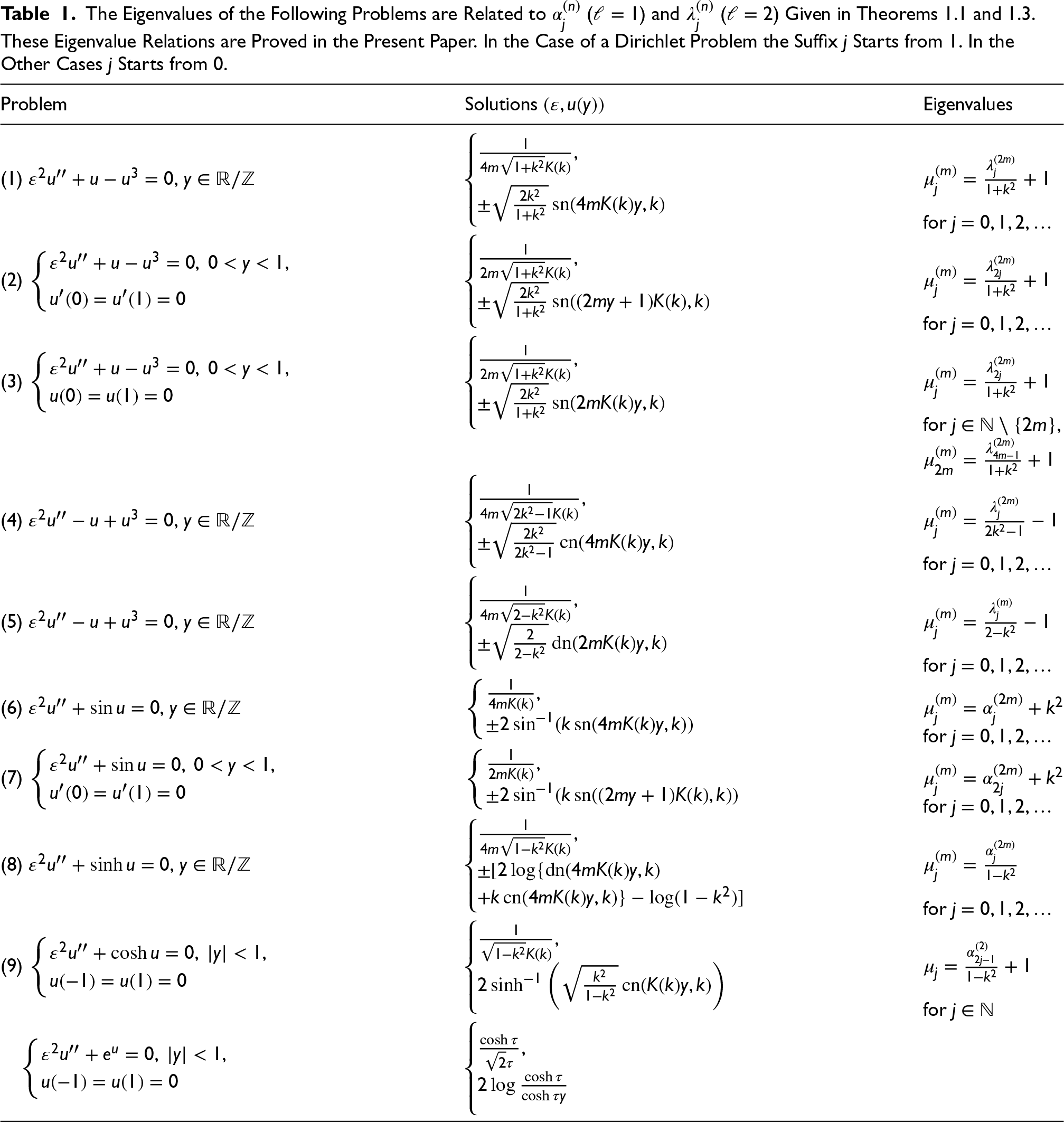
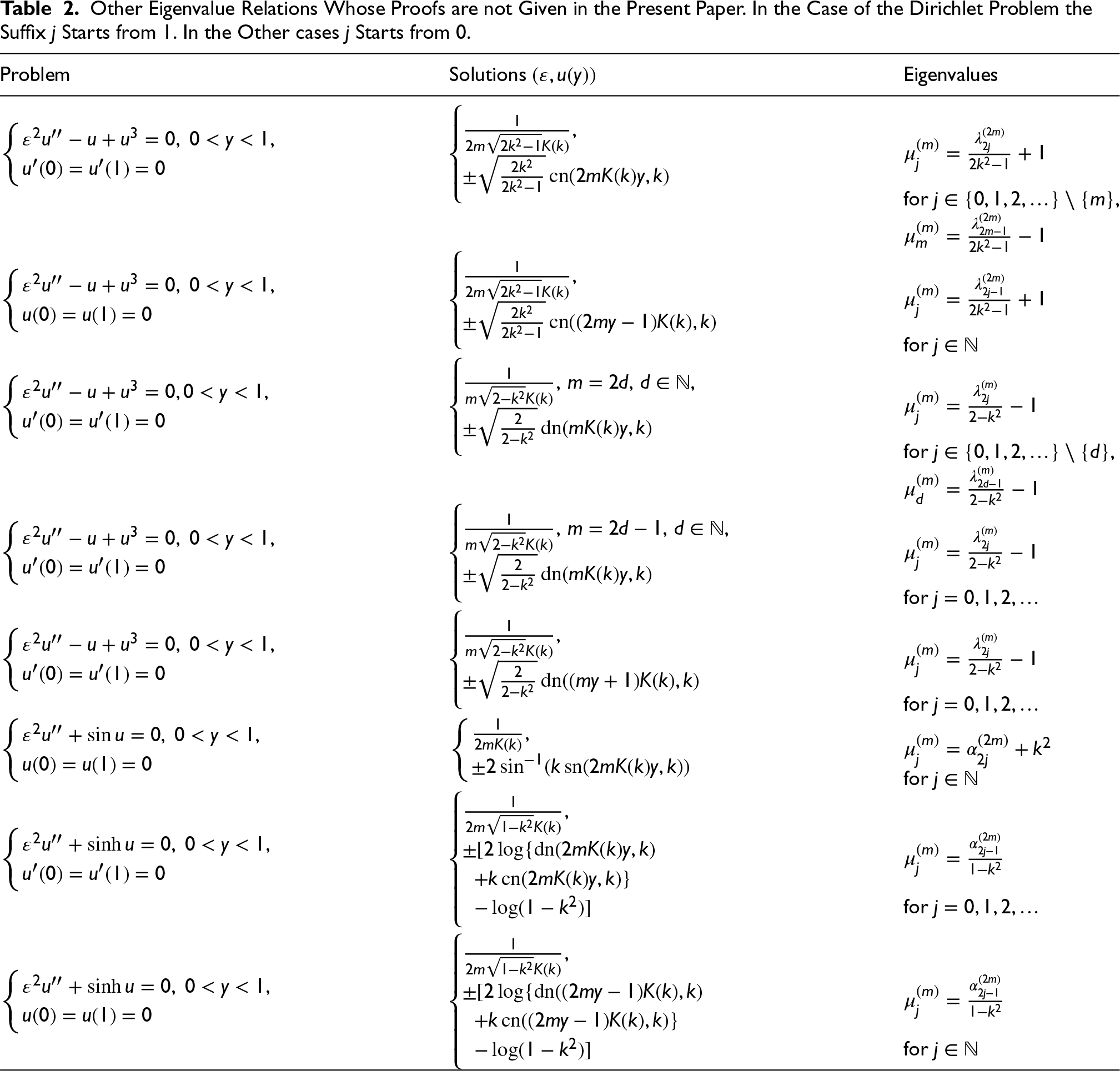
As seen in derivations of (1.13), (1.18) and (1.23), Theorems 1.1 and 1.3 with eigenvalue relations lead to asymptotic formulas for all eigenvalues as $ε \to 0$ . The third main result is eigenvalue relations given in Tables 1 and 2. Eigenvalue relations in Table 1 are proved in Section 6, but proofs of those of Table 2 are omitted. Explicit forms of asymptotic formulas as $ε \to 0$ are omitted, since it can be calculated in the same way.

Table 1.
The Eigenvalues of the Following Problems are Related to $α_{j}^{(n)}$ ( $ℓ = 1$ ) and $λ_{j}^{(n)}$ ( $ℓ = 2$ ) Given in Theorems 1.1 and 1.3. These Eigenvalue Relations are Proved in the Present Paper. In the Case of a Dirichlet Problem the Suffix $j$ Starts from $1$ . In the Other Cases $j$ Starts from $0$ .

Problem Solutions $(ε, u (y))$ Eigenvalues

(1) $ε^{2} u^{″} + u - u^{3} = 0$ , $y \in R / Z$ ${\begin{cases} \frac{1}{4 m \sqrt{1 + k^{2}} K (k)}, \\ \pm \sqrt{\frac{2 k^{2}}{1 + k^{2}}} sn (4 m K (k) y, k) \end{cases}$ $μ_{j}^{(m)} = \frac{λ_{j}^{(2 m)}}{1 + k^{2}} + 1$

for $j = 0, 1, 2, \dots$

(2) ${\begin{cases} ε^{2} u^{″} + u - u^{3} = 0, 0 < y < 1, \\ u^{'} (0) = u^{'} (1) = 0 \end{cases}$ ${\begin{cases} \frac{1}{2 m \sqrt{1 + k^{2}} K (k)}, \\ \pm \sqrt{\frac{2 k^{2}}{1 + k^{2}}} sn ((2 m y + 1) K (k), k) \end{cases}$ $μ_{j}^{(m)} = \frac{λ_{2 j}^{(2 m)}}{1 + k^{2}} + 1$

for $j = 0, 1, 2, \dots$

(3) ${\begin{cases} ε^{2} u^{″} + u - u^{3} = 0, 0 < y < 1, \\ u (0) = u (1) = 0 \end{cases}$ ${\begin{cases} \frac{1}{2 m \sqrt{1 + k^{2}} K (k)}, \\ \pm \sqrt{\frac{2 k^{2}}{1 + k^{2}}} sn (2 m K (k) y, k) \end{cases}$ $μ_{j}^{(m)} = \frac{λ_{2 j}^{(2 m)}}{1 + k^{2}} + 1$

for $j \in N ∖ {2 m}$ ,

$μ_{2 m}^{(m)} = \frac{λ_{4 m - 1}^{(2 m)}}{1 + k^{2}} + 1$

(4) $ε^{2} u^{″} - u + u^{3} = 0$ , $y \in R / Z$ ${\begin{cases} \frac{1}{4 m \sqrt{2 k^{2} - 1} K (k)}, \\ \pm \sqrt{\frac{2 k^{2}}{2 k^{2} - 1}} cn (4 m K (k) y, k) \end{cases}$ $μ_{j}^{(m)} = \frac{λ_{j}^{(2 m)}}{2 k^{2} - 1} - 1$

for $j = 0, 1, 2, \dots$

(5) $ε^{2} u^{″} - u + u^{3} = 0$ , $y \in R / Z$ ${\begin{cases} \frac{1}{4 m \sqrt{2 - k^{2}} K (k)}, \\ \pm \sqrt{\frac{2}{2 - k^{2}}} dn (2 m K (k) y, k) \end{cases}$ $μ_{j}^{(m)} = \frac{λ_{j}^{(m)}}{2 - k^{2}} - 1$

for $j = 0, 1, 2, \dots$

(6) $ε^{2} u^{″} + \sin u = 0$ , $y \in R / Z$ ${\begin{cases} \frac{1}{4 m K (k)}, \\ \pm 2 \sin^{- 1} (k sn (4 m K (k) y, k)) \end{cases}$ $μ_{j}^{(m)} = α_{j}^{(2 m)} + k^{2}$

for $j = 0, 1, 2, \dots$

(7) ${\begin{cases} ε^{2} u^{″} + \sin u = 0, 0 < y < 1, \\ u^{'} (0) = u^{'} (1) = 0 \end{cases}$ ${\begin{cases} \frac{1}{2 m K (k)}, \\ \pm 2 \sin^{- 1} (k sn ((2 m y + 1) K (k), k)) \end{cases}$ $μ_{j}^{(m)} = α_{2 j}^{(2 m)} + k^{2}$

for $j = 0, 1, 2, \dots$

(8) $ε^{2} u^{″} + \sinh u = 0$ , $y \in R / Z$ ${\begin{cases} \frac{1}{4 m \sqrt{1 - k^{2}} K (k)}, \\ \pm [2 \log {dn (4 m K (k) y, k) \\ + k cn (4 m K (k) y, k)} - \log (1 - k^{2})] \end{cases}$ $μ_{j}^{(m)} = \frac{α_{j}^{(2 m)}}{1 - k^{2}}$

for $j = 0, 1, 2, \dots$

(9) ${\begin{cases} ε^{2} u^{″} + \cosh u = 0, | y | < 1, \\ u (- 1) = u (1) = 0 \end{cases}$ ${\begin{cases} \frac{1}{\sqrt{1 - k^{2}} K (k)}, \\ 2 \sinh^{- 1} (\sqrt{\frac{k^{2}}{1 - k^{2}}} cn (K (k) y, k)) \end{cases}$ $μ_{j} = \frac{α_{2 j - 1}^{(2)}}{1 - k^{2}} + 1$

for $j \in N$

${\begin{cases} ε^{2} u^{″} + e^{u} = 0, | y | < 1, \\ u (- 1) = u (1) = 0 \end{cases}$ ${\begin{cases} \frac{\cosh τ}{\sqrt{2} τ}, \\ 2 \log \frac{\cosh τ}{\cosh τ y} \end{cases}$

Table 2.
Other Eigenvalue Relations Whose Proofs are not Given in the Present Paper. In the Case of the Dirichlet Problem the Suffix $j$ Starts from $1$ . In the Other cases $j$ Starts from $0$ .

Problem Solutions $(ε, u (y))$ Eigenvalues

${\begin{cases} ε^{2} u^{″} - u + u^{3} = 0, 0 < y < 1, \\ u^{'} (0) = u^{'} (1) = 0 \end{cases}$ ${\begin{cases} \frac{1}{2 m \sqrt{2 k^{2} - 1} K (k)}, \\ \pm \sqrt{\frac{2 k^{2}}{2 k^{2} - 1}} cn (2 m K (k) y, k) \end{cases}$ $μ_{j}^{(m)} = \frac{λ_{2 j}^{(2 m)}}{2 k^{2} - 1} + 1$

for $j \in {0, 1, 2, \dots} ∖ {m}$ ,

$μ_{m}^{(m)} = \frac{λ_{2 m - 1}^{(2 m)}}{2 k^{2} - 1} - 1$

${\begin{cases} ε^{2} u^{″} - u + u^{3} = 0, 0 < y < 1, \\ u (0) = u (1) = 0 \end{cases}$ ${\begin{cases} \frac{1}{2 m \sqrt{2 k^{2} - 1} K (k)}, \\ \pm \sqrt{\frac{2 k^{2}}{2 k^{2} - 1}} cn ((2 m y - 1) K (k), k) \end{cases}$ $μ_{j}^{(m)} = \frac{λ_{2 j - 1}^{(2 m)}}{2 k^{2} - 1} + 1$

for $j \in N$

${\begin{cases} ε^{2} u^{″} - u + u^{3} = 0, 0 < y < 1, \\ u^{'} (0) = u^{'} (1) = 0 \end{cases}$ ${\begin{cases} \frac{1}{m \sqrt{2 - k^{2}} K (k)}, m = 2 d, d \in N, \\ \pm \sqrt{\frac{2}{2 - k^{2}}} dn (m K (k) y, k) \end{cases}$ $μ_{j}^{(m)} = \frac{λ_{2 j}^{(m)}}{2 - k^{2}} - 1$

for $j \in {0, 1, 2, \dots} ∖ {d}$ ,

$μ_{d}^{(m)} = \frac{λ_{2 d - 1}^{(m)}}{2 - k^{2}} - 1$

${\begin{cases} ε^{2} u^{″} - u + u^{3} = 0, 0 < y < 1, \\ u^{'} (0) = u^{'} (1) = 0 \end{cases}$ ${\begin{cases} \frac{1}{m \sqrt{2 - k^{2}} K (k)}, m = 2 d - 1, d \in N, \\ \pm \sqrt{\frac{2}{2 - k^{2}}} dn (m K (k) y, k) \end{cases}$ $μ_{j}^{(m)} = \frac{λ_{2 j}^{(m)}}{2 - k^{2}} - 1$

for $j = 0, 1, 2, \dots$

${\begin{cases} ε^{2} u^{″} - u + u^{3} = 0, 0 < y < 1, \\ u^{'} (0) = u^{'} (1) = 0 \end{cases}$ ${\begin{cases} \frac{1}{m \sqrt{2 - k^{2}} K (k)}, \\ \pm \sqrt{\frac{2}{2 - k^{2}}} dn ((m y + 1) K (k), k) \end{cases}$ $μ_{j}^{(m)} = \frac{λ_{2 j}^{(m)}}{2 - k^{2}} - 1$

for $j = 0, 1, 2, \dots$

${\begin{cases} ε^{2} u^{″} + \sin u = 0, 0 < y < 1, \\ u (0) = u (1) = 0 \end{cases}$ ${\begin{cases} \frac{1}{2 m K (k)}, \\ \pm 2 \sin^{- 1} (k sn (2 m K (k) y, k)) \end{cases}$ $μ_{j}^{(m)} = α_{2 j}^{(2 m)} + k^{2}$

for $j \in N$

${\begin{cases} ε^{2} u^{″} + \sinh u = 0, 0 < y < 1, \\ u^{'} (0) = u^{'} (1) = 0 \end{cases}$ ${\begin{cases} \frac{1}{2 m \sqrt{1 - k^{2}} K (k)}, \\ \pm [2 \log {dn (2 m K (k) y, k) \\ + k cn (2 m K (k) y, k)} \\ - \log (1 - k^{2})] \end{cases}$ $μ_{j}^{(m)} = \frac{α_{2 j - 1}^{(2 m)}}{1 - k^{2}}$

for $j = 0, 1, 2, \dots$

${\begin{cases} ε^{2} u^{″} + \sinh u = 0, 0 < y < 1, \\ u (0) = u (1) = 0 \end{cases}$ ${\begin{cases} \frac{1}{2 m \sqrt{1 - k^{2}} K (k)}, \\ \pm [2 \log {dn ((2 m y - 1) K (k), k) \\ + k cn ((2 m y - 1) K (k), k)} \\ - \log (1 - k^{2})] \end{cases}$ $μ_{j}^{(m)} = \frac{α_{2 j - 1}^{(2 m)}}{1 - k^{2}}$

for $j \in N$

The two equations $ε^{2} u^{″} + \sin u = 0$ ( $ℓ = 1$ ) and $ε^{2} u^{″} + u - u^{3} = 0$ ( $ℓ = 2$ ) became model cases. After (Wakasa & Yotsutani, 2008, 2015), the scalar field equation $ε^{2} u^{″} - u + u^{p} = 0$ with $p = 3$ was studied in Miyamoto et al. (2023). The scalar field equation has two families of solutions which can be expressed as $cn$ - and $dn$ -functions which are in (4) and (5) in Table 1. In Miyamoto et al. (2023) it was found that solutions of the $dn$ -function of the Neumann problem corresponded to the case $ℓ = 2$ and the asymptotic formula was established. In this article, we study the cases of a $cn$ - and $dn$ -function of the periodic boundary value problem. In Aizawa et al. (2023) the cases of $ε^{2} u^{″} + \sinh u = 0$ with Dirichlet and Neumann problems were studied. In this paper we study the case $ε^{2} u^{″} + \sinh u = 0$ with periodic boundary condition. The Dirichlet problem of $ε^{2} u^{″} + \cosh u = 0$ is also studied.

We study the Dirichlet problem of $ε^{2} u^{″} + e^{u} = 0$ which was already considered in Miyamoto and Wakasa (2019). Although the eigenvalue relation does not exist, this problem can be seen as the limit case $k \to 1$ of (1.2) in a certain sense. Lastly, we mention the case $ℓ = 3$ in Subsection 6.5. The equation (1.1) with $ℓ = 3$ appears in the linearization problem of $ε^{2} u^{″} - u + u^{2} = 0$ . Therefore, a counterpart of Theorem 1.1 (and 1.3) is required. However, the case $ℓ = 3$ is difficult, and it may be a future work. Eigenvalue relations about eight more problems are shown in Table 2. Their proofs are omitted.

Let us explain technical details. An integral representation of two independent solutions of the ODE in (1.1) is known (Proposition 2.13), and it is written explicitly when $ℓ = 1, 2$ . This representation is often written in terms of Weierstrass’s $℘$ function. In this paper we write the integral representation in terms of Jacobi’s elliptic function, using a relation between a $℘$ -function and $sn$ -function (Proposition 2.8). Combining the integral representation and a theory of Hill’s operator, we show a multiplicity of each eigenvalue of (1.1). In Wakasa and Yotsutani (2008, 2015) various limit formulas related to complete elliptic integrals were developed. Using those limit formulas, we prove Theorems 1.1 and 1.3.

This paper consists of seven sections. In Section 2 we recall a theory of Hill’s equation. We also collect useful properties of the Lamé equation. In particular, integral representations of two independent solutions are given. In Section 3 we prove a simplicity of the eigenvalues given in Theorems 1.1 (i) and 1.3 (i). In Sections 4 and 5 we prove Theorems 1.1 (ii) and 1.3 (ii), respectively. In Section 6 we prove the eigenvalue relations in Table 1. We also study the Dirichlet problem $ε^{2} u^{″} + e^{u} = 0$ in details. Section 7 is an appendix. We recall definitions and basic properties of complete elliptic integrals $K (k)$ , $E (k)$ and $Π (ν, k)$ and Jacobi’s elliptic functions $sn (x, k)$ , $cn (x, k)$ and $dn (x, k)$ . We also recall basic facts of Weierstrass’s elliptic function $℘ (z)$ . We collect various limit formulas for complete elliptic integrals.
2. Fundamental Results

Problem	Solutions $(ε, u (y))$	Eigenvalues
(1) $ε^{2} u^{″} + u - u^{3} = 0$ , $y \in R / Z$	${\begin{cases} \frac{1}{4 m \sqrt{1 + k^{2}} K (k)}, \\ \pm \sqrt{\frac{2 k^{2}}{1 + k^{2}}} sn (4 m K (k) y, k) \end{cases}$	$μ_{j}^{(m)} = \frac{λ_{j}^{(2 m)}}{1 + k^{2}} + 1$
		for $j = 0, 1, 2, \dots$
(2) ${\begin{cases} ε^{2} u^{″} + u - u^{3} = 0, 0 < y < 1, \\ u^{'} (0) = u^{'} (1) = 0 \end{cases}$	${\begin{cases} \frac{1}{2 m \sqrt{1 + k^{2}} K (k)}, \\ \pm \sqrt{\frac{2 k^{2}}{1 + k^{2}}} sn ((2 m y + 1) K (k), k) \end{cases}$	$μ_{j}^{(m)} = \frac{λ_{2 j}^{(2 m)}}{1 + k^{2}} + 1$
		for $j = 0, 1, 2, \dots$
(3) ${\begin{cases} ε^{2} u^{″} + u - u^{3} = 0, 0 < y < 1, \\ u (0) = u (1) = 0 \end{cases}$	${\begin{cases} \frac{1}{2 m \sqrt{1 + k^{2}} K (k)}, \\ \pm \sqrt{\frac{2 k^{2}}{1 + k^{2}}} sn (2 m K (k) y, k) \end{cases}$	$μ_{j}^{(m)} = \frac{λ_{2 j}^{(2 m)}}{1 + k^{2}} + 1$
		for $j \in N ∖ {2 m}$ ,
		$μ_{2 m}^{(m)} = \frac{λ_{4 m - 1}^{(2 m)}}{1 + k^{2}} + 1$
(4) $ε^{2} u^{″} - u + u^{3} = 0$ , $y \in R / Z$	${\begin{cases} \frac{1}{4 m \sqrt{2 k^{2} - 1} K (k)}, \\ \pm \sqrt{\frac{2 k^{2}}{2 k^{2} - 1}} cn (4 m K (k) y, k) \end{cases}$	$μ_{j}^{(m)} = \frac{λ_{j}^{(2 m)}}{2 k^{2} - 1} - 1$
		for $j = 0, 1, 2, \dots$
(5) $ε^{2} u^{″} - u + u^{3} = 0$ , $y \in R / Z$	${\begin{cases} \frac{1}{4 m \sqrt{2 - k^{2}} K (k)}, \\ \pm \sqrt{\frac{2}{2 - k^{2}}} dn (2 m K (k) y, k) \end{cases}$	$μ_{j}^{(m)} = \frac{λ_{j}^{(m)}}{2 - k^{2}} - 1$
		for $j = 0, 1, 2, \dots$
(6) $ε^{2} u^{″} + \sin u = 0$ , $y \in R / Z$	${\begin{cases} \frac{1}{4 m K (k)}, \\ \pm 2 \sin^{- 1} (k sn (4 m K (k) y, k)) \end{cases}$	$μ_{j}^{(m)} = α_{j}^{(2 m)} + k^{2}$
		for $j = 0, 1, 2, \dots$
(7) ${\begin{cases} ε^{2} u^{″} + \sin u = 0, 0 < y < 1, \\ u^{'} (0) = u^{'} (1) = 0 \end{cases}$	${\begin{cases} \frac{1}{2 m K (k)}, \\ \pm 2 \sin^{- 1} (k sn ((2 m y + 1) K (k), k)) \end{cases}$	$μ_{j}^{(m)} = α_{2 j}^{(2 m)} + k^{2}$
		for $j = 0, 1, 2, \dots$
(8) $ε^{2} u^{″} + \sinh u = 0$ , $y \in R / Z$	${\begin{cases} \frac{1}{4 m \sqrt{1 - k^{2}} K (k)}, \\ \pm [2 \log {dn (4 m K (k) y, k) \\ + k cn (4 m K (k) y, k)} - \log (1 - k^{2})] \end{cases}$	$μ_{j}^{(m)} = \frac{α_{j}^{(2 m)}}{1 - k^{2}}$
		for $j = 0, 1, 2, \dots$
(9) ${\begin{cases} ε^{2} u^{″} + \cosh u = 0, \| y \| < 1, \\ u (- 1) = u (1) = 0 \end{cases}$	${\begin{cases} \frac{1}{\sqrt{1 - k^{2}} K (k)}, \\ 2 \sinh^{- 1} (\sqrt{\frac{k^{2}}{1 - k^{2}}} cn (K (k) y, k)) \end{cases}$	$μ_{j} = \frac{α_{2 j - 1}^{(2)}}{1 - k^{2}} + 1$
		for $j \in N$
${\begin{cases} ε^{2} u^{″} + e^{u} = 0, \| y \| < 1, \\ u (- 1) = u (1) = 0 \end{cases}$	${\begin{cases} \frac{\cosh τ}{\sqrt{2} τ}, \\ 2 \log \frac{\cosh τ}{\cosh τ y} \end{cases}$

Problem	Solutions $(ε, u (y))$	Eigenvalues
${\begin{cases} ε^{2} u^{″} - u + u^{3} = 0, 0 < y < 1, \\ u^{'} (0) = u^{'} (1) = 0 \end{cases}$	${\begin{cases} \frac{1}{2 m \sqrt{2 k^{2} - 1} K (k)}, \\ \pm \sqrt{\frac{2 k^{2}}{2 k^{2} - 1}} cn (2 m K (k) y, k) \end{cases}$	$μ_{j}^{(m)} = \frac{λ_{2 j}^{(2 m)}}{2 k^{2} - 1} + 1$
		for $j \in {0, 1, 2, \dots} ∖ {m}$ ,
		$μ_{m}^{(m)} = \frac{λ_{2 m - 1}^{(2 m)}}{2 k^{2} - 1} - 1$
${\begin{cases} ε^{2} u^{″} - u + u^{3} = 0, 0 < y < 1, \\ u (0) = u (1) = 0 \end{cases}$	${\begin{cases} \frac{1}{2 m \sqrt{2 k^{2} - 1} K (k)}, \\ \pm \sqrt{\frac{2 k^{2}}{2 k^{2} - 1}} cn ((2 m y - 1) K (k), k) \end{cases}$	$μ_{j}^{(m)} = \frac{λ_{2 j - 1}^{(2 m)}}{2 k^{2} - 1} + 1$
		for $j \in N$
${\begin{cases} ε^{2} u^{″} - u + u^{3} = 0, 0 < y < 1, \\ u^{'} (0) = u^{'} (1) = 0 \end{cases}$	${\begin{cases} \frac{1}{m \sqrt{2 - k^{2}} K (k)}, m = 2 d, d \in N, \\ \pm \sqrt{\frac{2}{2 - k^{2}}} dn (m K (k) y, k) \end{cases}$	$μ_{j}^{(m)} = \frac{λ_{2 j}^{(m)}}{2 - k^{2}} - 1$
		for $j \in {0, 1, 2, \dots} ∖ {d}$ ,
		$μ_{d}^{(m)} = \frac{λ_{2 d - 1}^{(m)}}{2 - k^{2}} - 1$
${\begin{cases} ε^{2} u^{″} - u + u^{3} = 0, 0 < y < 1, \\ u^{'} (0) = u^{'} (1) = 0 \end{cases}$	${\begin{cases} \frac{1}{m \sqrt{2 - k^{2}} K (k)}, m = 2 d - 1, d \in N, \\ \pm \sqrt{\frac{2}{2 - k^{2}}} dn (m K (k) y, k) \end{cases}$	$μ_{j}^{(m)} = \frac{λ_{2 j}^{(m)}}{2 - k^{2}} - 1$
		for $j = 0, 1, 2, \dots$
${\begin{cases} ε^{2} u^{″} - u + u^{3} = 0, 0 < y < 1, \\ u^{'} (0) = u^{'} (1) = 0 \end{cases}$	${\begin{cases} \frac{1}{m \sqrt{2 - k^{2}} K (k)}, \\ \pm \sqrt{\frac{2}{2 - k^{2}}} dn ((m y + 1) K (k), k) \end{cases}$	$μ_{j}^{(m)} = \frac{λ_{2 j}^{(m)}}{2 - k^{2}} - 1$
		for $j = 0, 1, 2, \dots$
${\begin{cases} ε^{2} u^{″} + \sin u = 0, 0 < y < 1, \\ u (0) = u (1) = 0 \end{cases}$	${\begin{cases} \frac{1}{2 m K (k)}, \\ \pm 2 \sin^{- 1} (k sn (2 m K (k) y, k)) \end{cases}$	$μ_{j}^{(m)} = α_{2 j}^{(2 m)} + k^{2}$
		for $j \in N$
${\begin{cases} ε^{2} u^{″} + \sinh u = 0, 0 < y < 1, \\ u^{'} (0) = u^{'} (1) = 0 \end{cases}$	${\begin{cases} \frac{1}{2 m \sqrt{1 - k^{2}} K (k)}, \\ \pm [2 \log {dn (2 m K (k) y, k) \\ + k cn (2 m K (k) y, k)} \\ - \log (1 - k^{2})] \end{cases}$	$μ_{j}^{(m)} = \frac{α_{2 j - 1}^{(2 m)}}{1 - k^{2}}$
		for $j = 0, 1, 2, \dots$
${\begin{cases} ε^{2} u^{″} + \sinh u = 0, 0 < y < 1, \\ u (0) = u (1) = 0 \end{cases}$	${\begin{cases} \frac{1}{2 m \sqrt{1 - k^{2}} K (k)}, \\ \pm [2 \log {dn ((2 m y - 1) K (k), k) \\ + k cn ((2 m y - 1) K (k), k)} \\ - \log (1 - k^{2})] \end{cases}$	$μ_{j}^{(m)} = \frac{α_{2 j - 1}^{(2 m)}}{1 - k^{2}}$
		for $j \in N$

2.1. Hill’s Equation

We recall a theory of Hill’s operator. Details can be found in Magnus and Winkler (1966, Part I in pp.3–48). Let $q (x)$ be a smooth $2 K (k)$ -periodic function and let $L := - \frac{d^{2}}{d x^{2}} + q (x)$ . We consider the problem

\begin{aligned} L ϕ = κ ϕ for x \in R . \end{aligned}

There exists a sequence

{κ_{j}}_{j = 0}^{\infty}

such that

\begin{aligned} - \infty = κ_{- 1} < κ_{0} < κ_{1} \leq κ_{2} < κ_{3} \leq κ_{4} < κ_{5} \leq κ_{6} < κ_{7} \leq \dots . \end{aligned}

κ \in (κ_{2 m - 1}, κ_{2 m})

m = 0, 1, 2, \dots

, then all nontrivial solutions are unbounded. We call

(κ_{2 m - 1}, κ_{2 m})

the interval of instability. On the other hand, if

κ \in (κ_{2 m}, κ_{2 m + 1})

m = 0, 1, 2, \dots

, then all solutions are bounded. We call

(κ_{2 m}, κ_{2 m + 1})

the interval of stability. If

κ = κ_{j}

for

j \geq 0

, then there exists a periodic solution with period

2 K (k)

4 K (k)

which is bounded. In this case a boundedness of a solution independent of the periodic one is as follows: If

κ_{2 m - 1} = κ_{2 m}

, then all solutions for

κ = κ_{2 m - 1} = κ_{2 m}

are bounded, and hence two adjacent intervals of stability

(κ_{2 m - 2}, κ_{2 m - 1})

and

(κ_{2 m}, κ_{2 m + 1})

can combine to a single one

(κ_{2 m - 2}, κ_{2 m + 1})

. In the other case

κ (= κ_{j})

is a boundary point of an interval of stability and also an interval of instability. Then a solution independent of a periodic one is unbounded. Thus, we obtain the following proposition.

Proposition 2.1
There exists a subsequence ${{\tilde{κ}}_{j}}_{j = 0}^{\infty}$ of ${κ_{j}}_{j = 0}^{\infty}$ , which may be a finite subsequence, such that ${\tilde{κ}}_{0} < {\tilde{κ}}_{1} < {\tilde{κ}}_{2} < \dots$ and the following (i)–(iii) hold:

(i) The intervals of stability is $({\tilde{κ}}_{0}, {\tilde{κ}}_{1}) \cup ({\tilde{κ}}_{2}, {\tilde{κ}}_{3}) \cup \dots \cup ({\tilde{κ}}_{2 m}, {\tilde{κ}}_{2 m + 1}) \cup \dots$ . If the subsequence is finite, then the last interval is $({\tilde{κ}}_{2 m}, \infty)$ .

(ii) The intervals of instability is $(- \infty, {\tilde{κ}}_{0}) \cup ({\tilde{κ}}_{1}, {\tilde{κ}}_{2}) \cup \dots \cup ({\tilde{κ}}_{2 m - 1}, {\tilde{κ}}_{2 m}) \cup \dots$ .

(iii) If $κ = {\tilde{κ}}_{j}$ , $j \geq 0$ , then a periodic (and bounded) solution exists and all solutions independent of the periodic one are unbounded.

In Magnus and Winkler (1966) the interval of the instability is defined as the complement of the intervals of stability in $R$ . In this paper we adopt a different definition of the interval of instability, which is based on Proposition 2.1.
2.2. The Lamé Equation on $C$

Let $ℓ$ be a positive integer. Let $Φ (z)$ , $z \in C$ , be a complex-valued function. We consider the Lamé equation of the form

\begin{aligned} - \frac{d^{2}}{d z^{2}} Φ + ℓ (ℓ + 1) ℘ (z; 2 ω_{1}, 2 ω_{3}) Φ = λ Φ, \end{aligned}

(2.1)

where

\begin{aligned} ω_{1} = K (k), ω_{3} = K (\sqrt{1 - k^{2}}) \sqrt{- 1}, 0 < k < 1 \end{aligned}

and

℘ (z; 2 ω_{1}, 2 ω_{3})

denotes Weierstrass’s elliptic function. A definition and basic properties of

℘ (z)

are summarized in Subsection 7.3.

We recall known results about (2.1). Propositions in this subsection are valid for more general equations. However, we restrict ourselves to the Lamé equation. Let $h (z)$ be the product of a pair of solutions of (2.1). Then $h (x)$ satisfies

\begin{aligned} \frac{d^{3}}{d z^{3}} h - 4 {ℓ (ℓ + 1) ℘ (z) - λ} \frac{d}{d z} h - 2 ℓ (ℓ + 1) ℘^{'} (z) h = 0. \end{aligned}

(2.2)

Proposition 2.2 Takemura, 2003, Proposition 3.5

For $ℓ \geq 1$ , (2.2) has a solution

\begin{aligned} Ξ (z, λ) = c_{0} (λ) + \sum_{j = 0}^{ℓ - 1} b_{j} (λ) ℘ {(z)}^{ℓ - j}, \end{aligned}

where

c_{0} (λ)

and

b_{j} (λ)

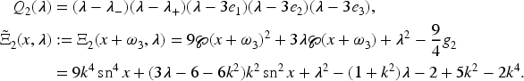
are polynomials in

λ

, they do not have common divisors and the polynomial

c_{0} (λ)

is monic. Moreover, the degree of

c_{0} (λ)

ℓ

and the degree of

b_{j} (λ)

is not more than

ℓ - 1

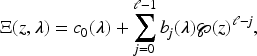
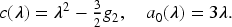
Let

\begin{aligned} Q (λ) := Ξ (z, λ)^{2} {λ - ℓ (ℓ + 1) ℘ (z)} + \frac{1}{2} Ξ (z, λ) \frac{d^{2} Ξ (z, λ)}{d z^{2}} - \frac{1}{4} {(\frac{d Ξ (z, λ)}{d z})}^{2} . \end{aligned}

(2.3)

Then the RHS is independent of

z

and it is a monic polynomial in

λ

of degree

2 ℓ + 1

. We can construct a solution of (2.1), using

Ξ (z, λ)

and

Q (λ)

Proposition 2.3 Takemura, 2003, Proposition 3.7

Let $Ξ (z, λ)$ be given by Proposition 2.2 and let $Q (λ)$ be given by (2.3). Then

\begin{aligned} Φ (z, λ) = \sqrt{Ξ (z, λ)} \exp \int \frac{\sqrt{- Q (λ)}}{Ξ (ζ, λ)} d ζ \end{aligned}

(2.4)

is a solution of (2.1).

The same expression as (2.4) appears in Whittaker and Watson (1927).

Example 2.4

Let $ω_{2} := - ω_{1} - ω_{3}$ and let

\begin{aligned} e_{1} := ℘ (ω_{1}) = \frac{2 - k^{2}}{3} > 0, e_{2} := ℘ (ω_{2}) = \frac{- 1 + 2 k^{2}}{3}, e_{3} := ℘ (ω_{3}) = \frac{- 1 - k^{2}}{3} < 0. \end{aligned}

(i) The case

ℓ = 1

\begin{aligned} Q_{1} (λ) = (λ + e_{1}) (λ + e_{2}) (λ + e_{3}), Ξ_{1} (z, λ) = ℘ (z) + λ . \end{aligned}

(ii) The case

ℓ = 2

\begin{aligned} Q_{2} (λ) = (λ^{2} - 3 g_{2}) (λ - 3 e_{1}) (λ - 3 e_{2}) (λ - 3 e_{3}), Ξ_{2} (z, λ) = 9 ℘ {(z)}^{2} + 3 λ ℘ (z) + λ^{2} - \frac{9}{4} g_{2}, \end{aligned}

where

g_{2} := - 4 (e_{1} e_{2} + e_{2} e_{3} + e_{3} e_{1}) = \frac{4}{3} (1 - k^{2} + k^{4})

(iii) The case $ℓ = 3$ ,

\begin{aligned} Q_{3} (λ) & = λ (λ^{2} + 6 e_{1} λ + 45 e_{1}^{2} - 15 g_{2}) (λ^{2} + 6 e_{2} λ + 45 e_{2}^{2} - 15 g_{2}) (λ^{2} + 6 e_{3} λ + 45 e_{3}^{2} - 15 g_{2}), \\ Ξ_{3} (z, λ) & = 225 ℘ {(z)}^{3} + 45 λ ℘ {(z)}^{2} + 6 (λ^{2} - \frac{75}{8} g_{2}) ℘ (z) + λ^{3} - 15 g_{2} λ - \frac{225}{4} g_{3}, \end{aligned}

where

g_{3} := 4 e_{1} e_{2} e_{3} = \frac{4}{27} (2 - k^{2}) (1 - 2 k^{2}) (1 + k^{2})

The cases $ℓ = 1, 2, 3$ in Example 2.4 correspond to $(ℓ_{0}, ℓ_{1}, ℓ_{2}, ℓ_{3}) = (1, 0, 0, 0)$ , $(2, 0, 0, 0)$ , $(3, 0, 0, 0)$ in Takemura (2005, Section 6), respectively. These formulas also can be found in Takemura (2006, Example 1 in p.107) and Takemura (2007).

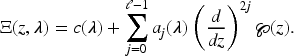
We rewrite the function $Ξ (z, λ)$ as follows:

\begin{aligned} Ξ (z, λ) = c (λ) + \sum_{j = 0}^{ℓ - 1} a_{j} (λ) {(\frac{d}{d z})}^{2 j} ℘ (z) . \end{aligned}

Then,

c (λ)

and

a_{j} (λ)

are polynomials in

λ

, and it follows from Proposition 2.2 that the degree of

c (λ)

ℓ

and the degree of

a_{j} (λ)

is not more than

ℓ - 1

Proposition 2.5

Takemura (2004, 2005) Let $λ^{'}$ be the eigenvalue satisfying $Q (λ^{'}) = 0$ . Then there exist $p \in {0, 1}$ such that $Φ (z + 2 ω_{1}, λ^{'}) = (- 1)^{p} Φ (z, λ^{'})$ , and we have

\begin{aligned} Φ (z + 2 ω_{1}, λ) = (- 1)^{p} Φ (z, λ) \exp (- \frac{1}{2} \int_{λ^{'}}^{λ} \frac{2 ω_{1} c (μ) - 2 η_{1} a_{0} (μ)}{\sqrt{- Q (μ)}} d μ), \end{aligned}

(2.5)

for any

λ

, where

η_{1} = ζ (ω_{1})

and

ζ (x)

is the Weierstrass zeta function.

Example 2.6

(i) The case $ℓ = 1$ . The value $λ^{'} = - e_{1}$ satisfies $Q (λ^{'}) = 0$ and $p = 0$ . The polynomials $c (λ)$ and $a_{0} (λ)$ are calculated as

\begin{aligned} c (λ) = λ, a_{0} (λ) = 1. \end{aligned}

(ii) The case

ℓ = 2

. The values

λ^{'} = \pm \sqrt{3 g_{2}}

satisfy

Q (λ^{'}) = 0

and

p = 0

. We have

\begin{aligned} c (λ) = λ^{2} - \frac{3}{2} g_{2}, a_{0} (λ) = 3 λ . \end{aligned}

(iii) The case

ℓ = 3

. The value

λ^{'} = 0

satisfies

Q (λ^{'}) = 0

and

p = 0

. We have

\begin{aligned} c (λ) = λ^{3} - \frac{45}{4} g_{2} λ - \frac{135}{4} g_{3}, a_{0} (λ) = 6 (λ^{2} - \frac{15}{4} g_{2}) . \end{aligned}

Set $P (λ) = 2 ω_{1} c (λ) - 2 η_{1} a_{0} (λ)$ . Then, the degree of $P (λ)$ is $ℓ$ . If $ω_{1}$ and $ω_{3} / \sqrt{- 1}$ are positive numbers, then every coefficient of $P (λ)$ is real-valued and the polynomial $Q (λ)$ has $2 ℓ + 1$ distinct real roots (see Takemura, 2003, Proposition 3.3). Write

\begin{aligned} Q (λ) = (λ - Λ_{0}) (λ - Λ_{1}) \dots (λ - Λ_{2 ℓ}), \end{aligned}

where

Λ_{0} < Λ_{1} < \dots < Λ_{2 ℓ}

. It follows from (2.5) that

\begin{aligned} \exp (- \frac{1}{2} \int_{Λ_{j}}^{Λ_{j + 1}} \frac{P (λ)}{\sqrt{- Q (λ)}} d λ) \in {1, - 1} \end{aligned}

for

j = 0, 1, \dots, 2 ℓ

. Hence there exists an integer

N_{j}

such that

\begin{aligned} \int_{Λ_{j}}^{Λ_{j + 1}} \frac{P (λ)}{\sqrt{- Q (λ)}} d λ = 2 π \sqrt{- 1} N_{j} . \end{aligned}

(2.6)

Proposition 2.7

Assume that $ω_{1}$ and $ω_{3} / \sqrt{- 1}$ are positive numbers.

(i) We have

\begin{aligned} \int_{Λ_{2 j - 1}}^{Λ_{2 j}} \frac{P (λ)}{\sqrt{- Q (λ)}} d λ = 0, j = 1, \dots, ℓ . \end{aligned}

(2.7)

(ii) The polynomial

P (λ)

has

ℓ

distinct real roots

Λ_{1}^{(P)}, \dots, Λ_{ℓ}^{(P)}

which satisfies

Λ_{2 j - 1} < Λ_{j}^{(P)} < Λ_{2 j}

for

j = 1, \dots, ℓ

Proof.

If $Λ_{2 j - 1} < λ < Λ_{2 j}$ , then $- Q (λ) > 0$ and the integrant $P (λ) / \sqrt{- Q (λ)}$ is real-valued. Hence the integral in the left-hand side of (2.7) is real-valued for each $j = 1, \dots, ℓ$ . By combining with (2.6), we obtain (i).

If the polynomial $P (λ)$ does not have zero on the interval $(Λ_{2 j - 1}, Λ_{2 j})$ for some $j$ , then the sign of the value $P (λ) / \sqrt{- Q (λ)}$ is constant. Thus the integral in the left-hand side of (2.7) is non-zero, which contradicts to (i). Hence, the polynomial $P (λ)$ has a zero on the interval $(Λ_{2 j - 1}, Λ_{2 j})$ for any $j = 1, \dots, ℓ$ . Since the degree of the $P (λ)$ is $ℓ$ , we obtain the proposition.

2.3. The Lamé Equation on

R

The function $℘ (x)$ is a complex-valued function. However, it is known that if $z = x + ω_{3}$ and $x \in R$ , then $℘ (z) = ℘ (x + ω_{3})$ is a real-valued smooth function on $R$ . Therefore, we define

\begin{aligned} \tilde{℘} (x) := ℘ (x + ω_{3}; 2 ω_{1}, 2 ω_{3}) . \end{aligned}

Then,

\tilde{℘} (x)

is related to Jacobi’s elliptic function as follows:

Proposition 2.8
Let $0 < k < 1$ . Then,
$\begin{aligned} \tilde{℘} (x) = e_{3} + k^{2} {sn}^{2} (x, k) for x \in R . \end{aligned}$
(2.8)
Therefore, for $x \in R$ , $e_{3} \leq \tilde{℘} (x) \leq e_{2}$ ,

See Lawden (1989, Eq.(6.9.11) in p.163) for (2.8). This relation is crucial in this paper. Let $z = x + ω_{3}$ . Then, the problem (2.1) for $x \in R$ becomes
$\begin{aligned} - ϕ^{″} + ℓ (ℓ + 1) (e_{3} + k^{2} {sn}^{2} x) ϕ = λ ϕ for x \in R . \end{aligned}$
(2.9)
When $λ \in R$ , $Ξ (x + ω_{3}, λ)$ can be chosen as a real-valued function. In that case $Q (λ)$ is also a real number. Hereafter, we define $\tilde{Ξ} (x, λ) := Ξ (x + ω_{3}, λ)$ for $x \in R$ . Since $z = x + ω_{3}$ , by (2.3) we can easily check that the same $Q (λ)$ as (2.3) satisfies
$\begin{aligned} Q (λ) = \tilde{Ξ} (x, λ)^{2} {λ - ℓ (ℓ + 1) \tilde{℘} (x)} + \frac{1}{2} \tilde{Ξ} (x, λ) \frac{d^{2} \tilde{Ξ} (x, λ)}{d x^{2}} - \frac{1}{4} {(\frac{d \tilde{Ξ} (x, λ)}{d x})}^{2} . \end{aligned}$
(2.10)

Let $f_{1} (x)$ and $f_{2} (x)$ be a basis of analytic solutions to the differential equation
$\begin{aligned} - ϕ^{″} + ℓ (ℓ + 1) (e_{3} + k^{2} {sn}^{2} x) ϕ = λ ϕ \end{aligned}$
(2.11)
about $x = 0$ . Since the function $e_{3} + k^{2} {sn}^{2} x$ is analytic in the domain $D = {x \in C | | ℑ x | < | ℑ ω_{3} |}$ , the functions $f_{1} (x)$ and $f_{2} (x)$ are continued analytically on the domain $D$ . It follows from the periodicity that the functions $f_{1} (x + 2 ω_{1})$ and $f_{2} (x + 2 ω_{1})$ also satisfy the differential equation (2.11). Since $f_{1} (x)$ and $f_{2} (x)$ are a basis of solutions, there exist $a, b, c, d \in C$ such that
$\begin{aligned} f_{1} (x + 2 ω_{1}) = a f_{1} (x) + c f_{2} (x), f_{2} (x + 2 ω_{1}) = b f_{1} (x) + d f_{2} (x) . \end{aligned}$
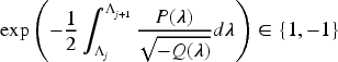
Then the values $a + d$ and $a d - b c$ do not depend on the choice of the basis $f_{1} (x)$ and $f_{2} (x)$ , and it is shown that $a d - b c = 1$ . Set
$\begin{aligned} Δ (λ) = a + d . \end{aligned}$
If $Δ (λ) > 2$ or $Δ (λ) < - 2$ , then any nonzero solutions are not bounded. If $- 2 < Δ (λ) < 2$ , then all solutions are bounded. If $Q (λ) \neq 0$ and $- 2 \leq Δ (λ) \leq 2$ , then all solutions are bounded. It follows from (2.5) that
$\begin{aligned} Δ (λ) = \pm {\exp (- \frac{1}{2} \int_{λ^{'}}^{λ} \frac{P (μ)}{\sqrt{- Q (μ)}} d μ) + \exp (\frac{1}{2} \int_{λ^{'}}^{λ} \frac{P (μ)}{\sqrt{- Q (μ)}} d μ)} . \end{aligned}$

Even or odd periodic solutions of (2.1) with period $2 K (k)$ or $4 K (k)$ are called the Lamé function.
Proposition 2.9
The following (i)–(iii) hold:

(i) If $Q (λ) > 0$ , then all solutions of (2.9) are bounded.

(ii) If $Q (λ) < 0$ , then all nontrivial solutions of (2.9) are unbounded.

(iii) If $Q (λ) = 0$ , then (2.9) has a periodic (and bounded) solution, which is the Lamé function, and all solutions independent of this solution are unbounded.

Proposition 2.9 seems to be known for experts. However, the authors could not find a proof in literature. Therefore, we show a proof.
Proof.
(i) If $λ \in R$ and $Q (λ) > 0$ , then $λ > Λ_{2 ℓ}$ or there exists $j \in {0, \dots, ℓ - 1}$ such that $Λ_{2 j} < λ < Λ_{2 j + 1}$ . In the case $λ > Λ_{2 ℓ}$ , we set $j = ℓ$ . It follows from (2.5) that
$\begin{aligned} Δ (λ) = \pm {\exp (- \frac{1}{2} \int_{Λ_{2 j}}^{λ} \frac{P (μ)}{\sqrt{- Q (μ)}} d μ) + \exp (\frac{1}{2} \int_{Λ_{2 j}}^{λ} \frac{P (μ)}{\sqrt{- Q (μ)}} d μ)} . \end{aligned}$
Since the integrant $P (μ) / \sqrt{- Q (μ)}$ is pure-imaginary for $Λ_{2 j} < μ < λ$ , we have $- 2 \leq Δ (λ) \leq 2$ . Hence, all solutions are bounded.

(ii) If $λ \in R$ and $Q (λ) < 0$ , then $λ < Λ_{0}$ or there exists $j \in {1, \dots, ℓ}$ such that $Λ_{2 j - 1} < λ < Λ_{2 j}$ . In the case $λ < Λ_{0}$ , we set $j = 0$ . Assume that $Λ_{2 j - 1} < λ \leq Λ_{j}^{(P)}$ It follows from (2.5) that
$\begin{aligned} Δ (λ) = \pm {\exp (- \frac{1}{2} \int_{Λ_{2 j - 1}}^{λ} \frac{P (μ)}{\sqrt{- Q (μ)}} d μ) + \exp (\frac{1}{2} \int_{Λ_{2 j - 1}}^{λ} \frac{P (μ)}{\sqrt{- Q (μ)}} d μ)} . \end{aligned}$
Since the integrant $P (μ) / \sqrt{- Q (μ)}$ is real and non-zero for $Λ_{2 j - 1} < μ < λ$ , we have $Δ (λ) < - 2$ or $Δ (λ) > 2$ . If $Λ_{j}^{(P)} < λ < Λ_{2 j}$ or $λ < Λ_{0}$ , then
$\begin{aligned} Δ (λ) = \pm {\exp (- \frac{1}{2} \int_{λ}^{Λ_{2 j}} \frac{P (μ)}{\sqrt{- Q (μ)}} d μ) + \exp (\frac{1}{2} \int_{λ}^{Λ_{2 j}} \frac{P (μ)}{\sqrt{- Q (μ)}} d μ)}, \end{aligned}$
the integrant $P (μ) / \sqrt{- Q (μ)}$ is real and non-zero, and we have $Δ (λ) < - 2$ or $Δ (λ) > 2$ . Therefore, any nonzero solutions are not bounded.

(iii) If $Q (λ) = 0$ , then the corresponding Lamé function is a solution. Since the degree of $Q (λ)$ is $2 ℓ + 1$ and $Q (λ)$ has $2 ℓ + 1$ different roots, each root is simple, and hence $λ$ is a boundary point of ${λ | Q (λ) > 0}$ and ${λ | Q (λ) < 0}$ . Because of (i) and (ii), $λ$ is a boundary point of the intervals of stability and also the intervals of instability. By Proposition 2.1 we see that all solutions independent of the Lamé function are unbounded.

If $ϕ (x)$ is an eigenfunction of (1.1), then $ϕ (x)$ can be regarded as a bounded periodic smooth function on $R$ , and hence $ϕ (x)$ is a bounded eigenfunction of (2.9). Thus, we obtain the following:
Proposition 2.10
All eigenvalues of (1.1) are on ${λ \in R; Q (λ) \geq 0}$ .

In the case of a Dirichlet (resp. Neumann) problem
$\begin{aligned} {\begin{cases} - ϕ^{″} + ℓ (ℓ + 1) (e_{3} + k^{2} {sn}^{2} x) ϕ = λ ϕ & for 0 < x < 2 K, \\ ϕ (0) = ϕ (2 K) = 0 (resp. ϕ^{'} (0) = ϕ^{'} (2 K) = 0) \end{cases} \end{aligned}$
an eigenfunction $ϕ (x)$ can be extended as a bounded periodic smooth function on $R$ by using odd reflection (resp. even reflection). Therefore, Proposition 2.10 holds for both Dirichlet and Neumann problems.

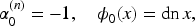
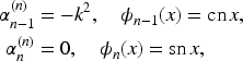
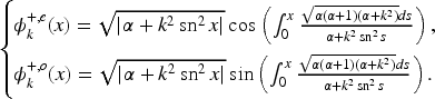
We study the case $Q (λ) = 0$ . In this case (2.9) has a periodic solution with period $2 K (k)$ or $4 K (k)$ called the Lamé function. The Lamé function can be expressed as a polynomial of $sn x$ , $cn x$ and $dn x$ . The following are examples of the Lamé function:
Example 2.11
(i) The case $ℓ = 1$ ,
$\begin{aligned} Λ_{0} = - e_{1}, ϕ (x) = dn x, Λ_{1} = - e_{2}, ϕ (x) = cn x, Λ_{2} = - e_{3}, ϕ (x) = sn x . \end{aligned}$
(ii) The case $ℓ = 2$ ,
$\begin{matrix} Λ_{0} = - \sqrt{3 g_{2}}, ϕ (x) = 1 + k^{2} + \sqrt{1 - k^{2} + k^{4}} - 3 k^{2} {sn}^{2} x \end{matrix}$

$\begin{matrix} Λ_{1} = 3 e_{3}, ϕ (x) = dn x cn x, Λ_{2} = 3 e_{2}, ϕ (x) = dn x sn x, Λ_{3} = 3 e_{1}, ϕ (x) = sn x cn x \end{matrix}$

$\begin{matrix} Λ_{4} = \sqrt{3 g_{2}}, ϕ (x) = 1 + k^{2} - \sqrt{1 - k^{2} + k^{4}} - 3 k^{2} {sn}^{2} x \end{matrix}$
Here,
$\begin{aligned} \sqrt{3 g_{2}} = 2 \sqrt{1 - k^{2} + k^{4}}, 3 e_{3} = - 1 - k^{2}, 3 e_{2} = - 1 + 2 k^{2}, 3 e_{1} = 2 - k^{2} . \end{aligned}$

The above examples can be found in Arscott (1964, p. 205).

Next we study the case $Q (λ) > 0$ .
Proposition 2.12
If $Q (λ) > 0$ , then $\tilde{Ξ} (x, λ)$ does not vanish on $x \in R$ .
Proof.
Suppose that $\tilde{Ξ} (x_{0}, λ) = 0$ . By (2.10) we have
$\begin{aligned} 0 < Q (λ) = - \frac{1}{4} {({\frac{d \tilde{Ξ} (x, λ)}{d x} |}_{x = x_{0}})}^{2} \leq 0, \end{aligned}$
which is a contradiction.

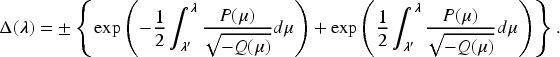
It follows from Proposition 2.12 that if $Q (λ) > 0$ , then $\tilde{Ξ} (x, λ)$ does not vanish or change sign. By Proposition 2.3 we can obtain two real-valued solutions defined for all $x \in R$ .
Proposition 2.13
Let $λ$ be such that $Q (λ) > 0$ . The following $ϕ^{e}$ and $ϕ^{o}$ are two independent solutions of (2.9) which are real-valued:
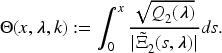
$\begin{aligned} ϕ^{e} (x) = \sqrt{| \tilde{Ξ} (x, λ) |} \cos (\int_{0}^{x} \frac{\sqrt{Q (λ)}}{| \tilde{Ξ} (s, λ) |} d s) and ϕ^{o} (x) = \sqrt{| \tilde{Ξ} (x, λ) |} \sin (\int_{0}^{x} \frac{\sqrt{Q (λ)}}{| \tilde{Ξ} (s, λ) |} d s) . \end{aligned}$

When we consider (1.1), the phase function $\int_{0}^{x} \frac{\sqrt{Q (λ)}}{| \tilde{Ξ} (s, λ) |} d s$ is important in checking the periodic boundary condition. In Sections 4 and 5 we study the phase function in detail.
2.4. The Lamée Equation on a Circle

We consider (1.1) as an eigenvalue problem.

Proposition 2.14
The following (i) and (ii) hold:

(i) If $λ$ is an eigenvalue and $Q (λ) = 0$ , then $λ$ is a simple eigenvalue and an eigenfunction is the Lamé function.

(ii) The other eigenvalues satisfy $Q (λ) > 0$ and have multiplicity $2$ . Moreover, $ϕ^{e}$ and $ϕ^{o}$ defined in Proposition 2.13 are two independent eigenfunctions.
Proof.
(i) Because of Proposition 2.9, all solutions independent of the Lamé function are unbounded on $R$ . Hence, the corresponding eigenfunction should be the Lamé function and the multiplicity of $λ$ is $1$ .

(ii) All eigenvalues other than (i) satisfy $Q (λ) > 0$ , because of Proposition 2.10. It follows from Proposition 2.13 that $ϕ^{e}$ and $ϕ^{o}$ are two independent eigenfunctions which have to be $2 n K (k)$ -periodic, and hence the multiplicity is at least $2$ . Since the equation of (1.1) is an ODE of the second order, the multiplicity is at most $2$ . Thus, the multiplicity is $2$ .
3. Simple Eigenvalues

In order to prove the simplicity of special eigenvalues we consider the following problem on $R$ :

\begin{aligned} - ϕ^{″} + (- 1 - k^{2} + 2 k^{2} {sn}^{2} x) ϕ = α ϕ for x \in R . \end{aligned}

(3.1)

Proof Proof of Theorem 1.1 (i).

By Example 2.11 we see that the following three pairs of $(α, ϕ (x))$ satisfy (3.1):

\begin{aligned} (- 1, dn x), (- k^{2}, cn x), (0, sn x) . \end{aligned}

It is obvious that

dn x

is a positive function in

X_{k}^{(n)}

. Thus,

- 1

is the first eigenvalue and hence the eigenvalue

- 1

is simple.

We consider the case where $n$ is even. Then, it is well known that the two pairs $(- k^{2}, cn x)$ and $(0, sn x)$ satisfy (1.2). Hence, they are eigenpairs. We see in the proof of Theorem 1.1 (ii) in Section 4 that (1.2) has $n - 1$ eigenvalues on ${α < - k^{2}}$ . Note that $2 [\frac{n - 1}{2}] + 1 = n - 1$ if $n$ is even. Thus, $- k^{2}$ is the $n$ -th eigenvalue, and hence $α_{n - 1} = - k^{2}$ . Since $cn x$ and $sn x$ have the same zero number on $X_{k}^{(n)}$ and $- k^{2} < 0$ , it follows from a Sturm–Liouville theory that $0$ is the eigenvalue next to $α_{n - 1}$ . Thus, $α_{n} = 0$ . It immediately follows from Proposition 2.14 that $α_{n - 1}$ and $α_{n}$ are simple eigenvalues.

We consider the case where $n$ is odd. This case is not mentioned in Theorem 1.1. The functions $cn x$ and $sn x$ are $4 K (k)$ -periodic and $2 n K (k)$ is not divisible by $4 K (k)$ . They are not solutions of (1.2). Therefore, neither $- k^{2}$ nor $0$ is an eigenvalue. The proof is complete.

We consider the following problem on $R$ :

\begin{aligned} - ϕ^{″} + (- 2 - 2 k^{2} + 6 k^{2} {sn}^{2} x) ϕ = λ ϕ for x \in R . \end{aligned}

(3.2)

Proof Proof of Theorem 1.3 (i).

By Example 2.11 (ii) we see that five pairs of $(λ, ϕ (x))$ satisfy (3.2). We easily check that $1 + k^{2} + \sqrt{1 - k^{2} + k^{4}} - 3 k^{2} {sn}^{2} x$ is positive for $x \in X_{k}^{(n)}$ . Thus, $- 2 \sqrt{1 - k^{2} + k^{4}}$ is the first eigenvalue, i.e., $λ_{0} = - 2 \sqrt{1 - k^{2} + k^{4}}$ .

We consider the case where $n$ is even. Using the same argument as in the proof of Theorem 1.1 (i), we can check that $- 1 - k^{2}$ is the $n$ -th eigenvalue and $- 1 + 2 k^{2}$ is the $n + 1$ -th eigenvalue, i.e., $λ_{n - 1} = - 1 - k^{2}$ and $λ_{n} = - 1 + 2 k^{2}$ . Note that neither $- 1 - k^{2}$ nor $- 1 + 2 k^{2}$ is an eigenvalue for odd $n$ , since both $cn x dn x$ and $sn x dn x$ are $4 K (k)$ -periodic functions and $2 n K (k)$ is not divisible by $4 K (k)$ .

Next we show that $λ_{2 n - 1} = 2 - k^{2}$ and $λ_{2 n} = 2 \sqrt{1 - k^{2} + k^{4}}$ . By proofs of Theorem 1.3 (ii) below we see that (1.4) has $2 n - 1$ eigenvalue on ${λ < 2 - k^{2}}$ whenever $n$ is odd or even. Thus, $2 - k^{2}$ is the $2 n$ -th eigenvalue, i.e., $λ_{2 n - 1} = 2 - k^{2}$ . We can easily check that $sn x cn x$ and $1 + k^{2} - \sqrt{1 - k^{2} + k^{4}} - 3 k^{2} {sn}^{2} x$ have the same zero number on $X_{k}^{(n)}$ . Thus, $2 \sqrt{1 - k^{2} + k^{4}}$ is the eigenvalue next to $λ_{2 n - 1}$ . i.e., $λ_{2 n} = 2 \sqrt{1 - k^{2} + k^{4}}$ . It follows from Proposition 2.14 that all eigenvalues associated with the Lamé functions are simple. The proof is complete.

4. Proof of Theorem 1.1

We consider the case $ℓ = 1$ . In this case it is convenient to study the following form:

\begin{aligned} - ϕ^{″} + (- 1 - k^{2} + 2 k^{2} {sn}^{2} x) ϕ = α ϕ for x \in X_{k}^{(n)}, \end{aligned}

(4.1)

where

α

is a new spectral parameter defined by

\begin{aligned} α = λ + e_{3} . \end{aligned}

The equation (4.1) is equivalent to (1.1) with

ℓ = 1

By Example 2.11 (i) we have

\begin{aligned} Q_{1} (λ) = & (λ + e_{1}) (λ + e_{2}) (λ + e_{3}) = α (α + 1) (α + k^{2}), \\ {\tilde{Ξ}}_{1} (x, α) := & Ξ_{1} (x + ω_{3}, λ) = ℘ (x + ω_{3}) + λ = α + k^{2} {sn}^{2} x . \end{aligned}

Then,

Q_{1} (λ) > 0

is equivalent to

\begin{aligned} α \in σ_{1} := (- 1, - k^{2}) \cup (0, \infty) . \end{aligned}

We find eigenvalues on

σ_{1}

. Proposition 2.12 guarantees that

{\tilde{Ξ}}_{1} (x, α)

does not vanish for

α \in σ_{1}

. It follows from Proposition 2.13 that the following

ϕ^{e}

and

ϕ^{o}

are two independent solutions of (3.1)

\begin{aligned} ϕ^{e} (x) := \sqrt{| α + k^{2} {sn}^{2} x |} \cos (Θ (x, α, k)) and ϕ^{o} (x) := \sqrt{| α + k^{2} {sn}^{2} x |} \sin (Θ (x, α, k)), \end{aligned}

(4.2)

where

\begin{aligned} Θ (x, α, k) := \int_{0}^{x} \frac{\sqrt{α (α + 1) (α + k^{2})}}{| α + k^{2} {sn}^{2} s |} d s . \end{aligned}

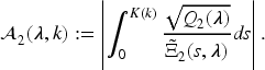
We define

\begin{aligned} M (α, k) := \int_{0}^{K (k)} \frac{\sqrt{α (α + 1) (α + k^{2})}}{α + k^{2} {sn}^{2} s} d s \end{aligned}

and

\begin{aligned} A (α, k) := | M (α, k) | . \end{aligned}

Since the integrand of

Θ

2 K (k)

-periodic, we see that

Θ (2 n K (k), α, k) = 2 n A (α, k)

. Therefore,

ϕ^{e}

and

ϕ^{o}

are solutions of (4.1) if and only if

\begin{aligned} 2 n A (α, k) = 2 π j for a nonnegative integer j . \end{aligned}

(4.3)

In this case

α

is an eigenvalue of (4.1) and the multiplicity is

2

. In this section we study

A (α, k)

to solve (4.3).

Lemma 4.1

For each fixed $k \in (0, 1)$ , the function $A (α, k)$ is continuous for $α \in σ_{1}$ .

Lemma 4.1 is obvious. The proof is omitted.

Lemma 4.2

The following hold:

(i) $lim_{α \to - 1^{+}} A (α, k) = 0$ .

(ii) $lim_{α \to (- k^{2})^{-}} A (α, k) = \frac{π}{2}$ .

(iii) $lim_{α \to 0^{+}} A (α, k) = \frac{π}{2}$ .

(iv) $lim_{α \to \infty} A (α, k) = \infty$ .

Proof.

The assertions (i), (ii), (iii), and (iv) follow from Lemma 7.2(i), (ii), (iii), and (iv), respectively.

Lemma 4.3

For each fixed $k \in (0, 1)$ , the function $A (α, k)$ is increasing for $α \in σ_{1}$ .

Proof.

Let $k \in (0, 1)$ be fixed. Let $θ (α) := A (α, k)$ and $ϕ := ϕ^{o}$ for simplicity. The function $ϕ (x)$ satisfies

\begin{aligned} {\begin{cases} ϕ^{″} + (α + 1 + k^{2} - 2 k^{2} {sn}^{2} x) ϕ = 0, & 0 < x < 2 n K (k), \\ ϕ (0) > 0, & ϕ^{'} (0) = 0 \end{cases} \end{aligned}

Since

ϕ

satisfies a Sturm–Liouville equation, we see that if

α

increases, then by Prüfer transformation

ϕ (x)

oscillates more rapidly. Hence,

(ϕ (2 n K (k)), ϕ^{'} (2 n K (k)))

rotates in the clockwise direction around the origin as

α

increases. Then,

θ (α)

is an increasing function on each connected component of

σ_{1}

. On the other hand,

θ (α)

is defined on

(- 1, - k^{2}) \cup (0, \infty)

. Because of Lemma 4.2 (ii) and (iii),

\begin{aligned} θ (α_{1}) < lim_{α \to - (k^{2})^{-}} θ (α) = \frac{π}{2} = lim_{α \to 0^{+}} θ (α) < θ (α_{2}) for α_{1} \in (- 1, - k^{2}) and α_{2} \in (0, \infty) . \end{aligned}

This indicates that

θ (α)

is an increasing function on the whole set of

σ_{1}

Proof Proof of Theorem 1.1 (ii).

Let $θ (α) := A (α, k)$ . Because of Lemmas 4.1–4.3, the continuous function $θ (α)$ is increasing in $α \in (- 1, - k^{2})$ , $lim_{α \to - 1} θ (α) = 0$ and $lim_{α \to - k^{2}} θ (α) = π / 2$ . Therefore, (4.3) has a unique solution for each $j \in {1, 2, \dots, [\frac{n - 1}{2}]}$ . Each solution gives arise an eigenvalue with multiplicity $2$ , and an associated eigenfunction has $2 j$ zeros in $X_{k}^{(n)}$ . Hence this eigenvalue is $α_{2 j - 1} = α_{2 j}$ .

First, we consider the case $α_{2 j - 1}^{(n)} (= α_{2 j}^{(n)})$ for $j \in {1, 2, \dots, [\frac{n - 1}{2}]}$ . Let $\tilde{α} = α_{2 j - 1}^{(n)} = α_{2 j}^{(n)}$ for simplicity. Then,

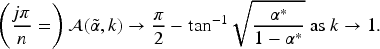
\begin{aligned} A (\tilde{α}, k) = \frac{j π}{n} . \end{aligned}

(4.4)

Lemmas 4.2 and 4.3 indicate that a solution

\tilde{α}

of (4.4) is unique and

- 1 < \tilde{α} < - k^{2}

. Hence,

\begin{aligned} 0 < \frac{- \tilde{α} - k^{2}}{1 - k^{2}} < 1. \end{aligned}

Letting

k \to 1

, we have a convergent subsequence of

\tilde{α}

which is still denoted by

\tilde{α}

. Then,

\begin{aligned} there exists α^{*} \in [0, 1] such that lim_{k \to 1} \frac{- \tilde{α} - k^{2}}{1 - k^{2}} = α^{*} . \end{aligned}

(4.5)

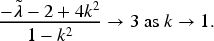
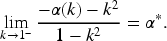
By Lemma 7.4 we have

\begin{aligned} (\frac{j π}{n} =) A (\tilde{α}, k) \to \frac{π}{2} - \tan^{- 1} \sqrt{\frac{α^{*}}{1 - α^{*}}} as k \to 1. \end{aligned}

Solving

\tan^{- 1} \sqrt{\frac{α^{*}}{1 - α^{*}}} = \frac{π}{2} - \frac{j π}{n}

with respect to

α^{*}

, we have

\begin{aligned} α^{*} = 1 - \sin^{2} (\frac{j π}{n}) . \end{aligned}

Note that the limit

α^{*}

is unique. By the limit in (4.5) we have

\begin{aligned} (α_{2 j - 1}^{(n)} = α_{2 j}^{(n)} =) \tilde{α} = - 1 + (\sin^{2} (\frac{j π}{n}) + o (1)) (1 - k^{2}) as k \to 1. \end{aligned}

Second, we consider the case $α_{2 j - 1}^{(n)} (= α_{2 j}^{(n)})$ for $j \in {[\frac{n + 2}{2}], [\frac{n + 2}{2}] + 1, \dots}$ . Because of Lemmas 4.2 and 4.3, the continuous function $θ (α)$ is increasing in $α \in (0, \infty)$ , $lim_{α \to 0} θ (α) = π / 2$ and $lim_{α \to \infty} θ (α) = \infty$ . Therefore, (4.3) has a unique solution for each $j \in {[\frac{n + 2}{2}], [\frac{n + 2}{2}] + 1, \dots}$ . By the same argument as in (ii) we see that the solution gives arise an eigenvalue with multiplicity $2$ which is denoted by $α_{2 j - 1}^{(n)} = α_{2 j}^{(n)}$ .

Let $\tilde{α} := α_{2 j - 1}^{(n)} = α_{2 j}^{(n)}$ for simplicity. Then,

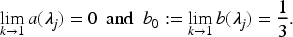
\begin{aligned} \frac{j π}{n} = A (\tilde{α}, k) \geq \int_{0}^{K (k)} \frac{\sqrt{\tilde{α} (\tilde{α} + k^{2}) (\tilde{α} + k^{2})}}{\tilde{α} + k^{2}} d s = \sqrt{\tilde{α}} K (k) . \end{aligned}

Therefore,

\sqrt{\tilde{α}} \leq \frac{j π}{n K (k)}

. We define

\begin{aligned} \hat{α} := \tilde{α} K {(k)}^{2} . \end{aligned}

(4.6)

Then,

0 \leq \sqrt{\hat{α}} \leq \frac{j π}{n}

. Letting

k \to 1

, we have a convergent subsequence of

\hat{α}

which is still denoted by

\hat{α}

. Then,

\begin{aligned} there exists {\hat{α}}^{*} \in [0, {(\frac{j π}{n})}^{2}] such that \hat{α} \to {\hat{α}}^{*} . \end{aligned}

(4.7)

We define

\begin{aligned} J (ν, k) := \int_{0}^{K (k)} \frac{\sqrt{ν + 1} d s}{1 + ν {sn}^{2} s} - \frac{1}{\sqrt{ν + 1}} K (k) . \end{aligned}

Let

ν = \frac{k^{2}}{\tilde{α}}

. Then,

\begin{aligned} \sqrt{\tilde{α} + 1} J (\frac{k^{2}}{\tilde{α}}, k) = \int_{0}^{K (k)} \frac{\sqrt{\tilde{α} (\tilde{α} + 1) (\tilde{α} + k^{2})}}{| \tilde{α} + k^{2} {sn}^{2} s |} d s - \sqrt{\frac{\tilde{α} (\tilde{α} + 1)}{\tilde{α} + k^{2}}} K (k) . \end{aligned}

(4.8)

Since

\tilde{α} \to 0

k \to 1

, we see that

\frac{k^{2}}{\tilde{α}} \to \infty

k \to 1

. By Lemma 7.3 we have

\begin{aligned} \sqrt{\tilde{α} + 1} J (\frac{k^{2}}{\tilde{α}}, k) \to \frac{π}{2} as k \to 1. \end{aligned}

(4.9)

Putting

\tilde{α} = \frac{\hat{α}}{K {(k)}^{2}}

into the last term of (4.8), we have

\begin{aligned} \sqrt{\frac{\tilde{α} (\tilde{α} + 1)}{\tilde{α} + k^{2}}} K (k) = \sqrt{\frac{\hat{α} (\frac{\hat{α}}{K {(k)}^{2}} + 1)}{\frac{\hat{α}}{K {(k)}^{2}} + k^{2}}} \to \sqrt{{\hat{α}}^{*}} as k \to 1. \end{aligned}

(4.10)

Letting

k \to 1

, by (4.8), (4.9) and (4.10) we have

\begin{aligned} \frac{π}{2} = \frac{j π}{n} - \sqrt{{\hat{α}}^{*}}, \end{aligned}

and hence

\begin{aligned} {\hat{α}}^{*} = \frac{(2 j - n)^{2} π^{2}}{4 n^{2}} . \end{aligned}

By (4.6) and (4.7) we have

\begin{aligned} (α_{2 j - 1}^{(n)} = α_{2 j}^{(n)} =) \tilde{α} = \frac{(2 j - n)^{2} π^{2}}{4 n^{2}} \frac{1}{K {(k)}^{2}} + o (\frac{1}{K {(k)}^{2}}) as k \to 1. \end{aligned}

The set

{α_{j}^{(n)}}_{j = 0}^{\infty}

consists of all the eigenvalues, since we have examined all

α \in closure (σ_{1})

in proofs of Theorem 1.1 (i) and (ii). Every eigenvalue in Theorem 1.1 (ii) has multiplicity

2

, since

ϕ^{e}

and

ϕ^{o}

are solutions of (4.1). The proof is complete.

5. Proof of Theorem 1.3

We consider the case $ℓ = 2$ , i.e.,

\begin{aligned} - ϕ^{″} + (- 2 - 2 k^{2} + 6 k^{2} {sn}^{2} x) ϕ = λ ϕ for x \in X_{k}^{(n)}, \end{aligned}

(5.1)

which is equivalent to (1.1) with

ℓ = 2

. Let us consider the problem (3.2). Let

\begin{aligned} λ_{-} := - 2 \sqrt{1 - k^{2} + k^{4}} and λ_{+} := 2 \sqrt{1 - k^{2} + k^{4}} . \end{aligned}

Since

3 g_{2} = 4 (1 - k^{2} + k^{4})

, by Example 2.11 (ii) we have

\begin{aligned} Q_{2} (λ) & = (λ - λ_{-}) (λ - λ_{+}) (λ - 3 e_{1}) (λ - 3 e_{2}) (λ - 3 e_{3}), \\ {\tilde{Ξ}}_{2} (x, λ) & := Ξ_{2} (x + ω_{3}, λ) = 9 ℘ (x + ω_{3})^{2} + 3 λ ℘ (x + ω_{3}) + λ^{2} - \frac{9}{4} g_{2} \\ = 9 k^{4} {sn}^{4} x + (3 λ - 6 - 6 k^{2}) k^{2} {sn}^{2} x + λ^{2} - (1 + k^{2}) λ - 2 + 5 k^{2} - 2 k^{4} . \end{aligned}

Then,

Q_{2} (λ) > 0

is equivalent to

\begin{aligned} λ \in σ_{2} := (λ_{-}, 3 e_{3}) \cup (3 e_{2}, 3 e_{1}) \cup (λ_{+}, \infty) . \end{aligned}

We find eigenvalues on

σ_{2}

. Proposition 2.12 guarantees that

{\tilde{Ξ}}_{2} (x, λ)

does not vanish for

λ \in σ_{2}

. It follows from Proposition 2.13 that the following

ϕ^{e}

and

ϕ^{o}

are two independent solutions of (3.2):

\begin{aligned} ϕ^{e} (x) := \sqrt{| {\tilde{Ξ}}_{2} (x, λ) |} \cos (Θ (x, λ, k)) and ϕ^{o} (x) := \sqrt{| {\tilde{Ξ}}_{2} (x, λ) |} \sin (Θ (x, λ, k)), \end{aligned}

where

\begin{aligned} Θ (x, λ, k) := \int_{0}^{x} \frac{\sqrt{Q_{2} (λ)}}{| {\tilde{Ξ}}_{2} (s, λ) |} d s . \end{aligned}

We define

\begin{aligned} A_{2} (λ, k) := | \int_{0}^{K (k)} \frac{\sqrt{Q_{2} (λ)}}{{\tilde{Ξ}}_{2} (s, λ)} d s | . \end{aligned}

It follows from the same argument as in the case

ℓ = 1

that

ϕ^{e}

and

ϕ^{o}

are solutions of (5.1) if and only if

\begin{aligned} 2 n A_{2} (λ, k) = 2 π j for a nonnegative integer j . \end{aligned}

We consider the case

\begin{aligned} λ \in (λ_{-}, 3 e_{3}) \cup (3 e_{2}, 3 e_{1}) . \end{aligned}

Then,

{\tilde{Ξ}}_{2} (x, λ)

can be factored as follows:

\begin{aligned} {\tilde{Ξ}}_{2} (x, λ) = 9 k^{4} (k^{2} {sn}^{2} x + α (λ)) (k^{2} {sn}^{2} x + β (λ)), \end{aligned}

where

\begin{aligned} α (λ) & = \frac{1}{6} [λ - 2 (1 + k^{2}) - \sqrt{3 {4 (1 - k^{2} + k^{4}) - λ^{2}}}], \\ β (λ) & = \frac{1}{6} [λ - 2 (1 + k^{2}) + \sqrt{3 {4 (1 - k^{2} + k^{4}) - λ^{2}}}] . \end{aligned}

Then, by direct calculation we obtain

\begin{aligned} \frac{\sqrt{Q_{2} (λ)}}{{\tilde{Ξ}}_{2} (x, λ)} = \frac{\sqrt{α (λ) (α (λ) + 1) (α (λ) + k^{2})}}{α (λ) + k^{2} {sn}^{2} s} - \frac{\sqrt{β (λ) (β (λ) + 1) (β (λ) + k^{2})}}{β (λ) + k^{2} {sn}^{2} s} . \end{aligned}

Thus, we obtain

\begin{aligned} A_{2} (λ, k) = | M (α (λ), k) - M (β (λ), k) | . \end{aligned}

Next, we consider the case

\begin{aligned} λ \in (λ_{+}, \infty) . \end{aligned}

Then,

{\tilde{Ξ}}_{2} (x, k)

cannot be factored.

Lemma 5.1

For each fixed $k \in (0, 1)$ , the function $A_{2} (λ, k)$ is continuous for $λ \in σ_{2}$ .

We omit the proof.

Lemma 5.2

The following hold:

(i) $lim_{λ \to (λ_{-})^{+}} A_{2} (λ, k) = 0$ .

(ii) $lim_{λ \to (3 e_{3})^{-}} A_{2} (λ, k) = \frac{π}{2}$ .

(iii) $lim_{λ \to (3 e_{2})^{+}} A_{2} (λ, k) = \frac{π}{2}$ .

(iv) $lim_{λ \to (3 e_{1})^{-}} A_{2} (λ, k) = π$ .

(v) $lim_{λ \to (λ_{+})^{+}} A_{2} (λ, k) = π$ .

(vi) $lim_{λ \to \infty} A_{2} (λ, k) = \infty$ .

Proof.

We omit signs of convergence.

(i) As $λ \to λ_{-}$ ,

\begin{aligned} α (λ) \to α (λ_{-}) = \frac{λ_{-} - 2 - 2 k^{2}}{6} and β (λ) \to β (λ_{-}) = \frac{λ_{-} - 2 - 2 k^{2}}{6}, \end{aligned}

and hence

α (λ_{-}) = β (λ_{-})

. Therefore,

\begin{aligned} lim_{λ \to λ_{-}} A_{2} (λ, k) = | M (α (λ_{-}), k) - M (β (λ_{-}), k) | = 0. \end{aligned}

(ii) As

λ \to 3 e_{3}

\begin{aligned} α (λ) \to - 1 and β (λ) \to - k^{2} . \end{aligned}

By Lemma 7.2 (i) and (ii) we have

\begin{aligned} lim_{λ \to 3 e_{3}} A_{2} (λ, k) = lim_{λ \to 3 e_{3}} | M (α (λ, k) - M (β (λ), k) | = | 0 - (- \frac{π}{2}) | = \frac{π}{2} . \end{aligned}

(iii) As

λ \to 3 e_{2}

\begin{aligned} α (λ) \to - 1 and β (λ) \to 0. \end{aligned}

By Lemma 7.2 (i) and (iii) we have

\begin{aligned} lim_{λ \to 3 e_{2}} A_{2} (λ, k) = lim_{λ \to 3 e_{2}} | M (α (λ, k) - M (β (λ), k) | = | 0 - \frac{π}{2} | = \frac{π}{2} . \end{aligned}

(iv) As

λ \to 3 e_{1}

\begin{aligned} α (λ) \to - k^{2} and β (λ) \to 0. \end{aligned}

By Lemma 7.2 (ii) and (iii) we have

\begin{aligned} lim_{λ \to 3 e_{1}} A_{2} (λ, k) = lim_{λ \to 3 e_{1}} | M (α (λ, k) - M (β (λ), k) | = | - \frac{π}{2} - \frac{π}{2} | = π . \end{aligned}

(v) Let

\begin{aligned} a (λ) := \frac{1}{12 k^{4}} {λ^{2} - 4 (1 - k^{2} + k^{4})} and b (λ) := \frac{- 1}{6 k^{2}} (λ - 2 - 2 k^{2}) . \end{aligned}

Then,

\begin{aligned} A_{2} (λ, k) = \frac{2 \sqrt{3 (λ - 3 e_{1}) (λ - 3 e_{2}) (λ - 3 e_{3})}}{9 k^{2}} \int_{0}^{K (k)} \frac{\sqrt{a (λ)} d s}{a (λ) + (b (λ) - {sn}^{2} s)^{2}} . \end{aligned}

λ \to λ_{+}

\begin{aligned} a (λ) \to 0 and b (λ) \to b_{0} := \frac{- 1}{6 k^{2}} (λ_{+} + 6 e_{3}) . \end{aligned}

By Lemma 7.5 we have

\begin{aligned} lim_{λ \to λ_{+}} A_{2} (λ, k) = \frac{2 \sqrt{3 (λ_{+} - 3 e_{1}) (λ_{+} - 3 e_{2}) (λ_{+} - 3 e_{3})}}{9 k^{2}} \frac{π}{2 \sqrt{b_{0} (1 - b_{0}) (1 - k^{2} b_{0})}} . \end{aligned}

Using

λ_{+} = \sqrt{3 g_{2}}

g_{2} = - 4 (e_{1} e_{2} + e_{2} e_{3} + e_{3} e_{1})

and

e_{1} + e_{2} + e_{3} = 0

, we have

\begin{aligned} \frac{2 \sqrt{3}}{9 k^{2}} \sqrt{(λ_{+} - 3 e_{1}) (λ_{+} - 3 e_{2}) (λ_{+} - 3 e_{3})} = & \frac{2 \sqrt{3}}{9 k^{2}} {λ_{+}^{3} + 9 (e_{1} e_{2} + e_{2} e_{3} + e_{3} e_{1}) λ_{+} - 27 e_{1} e_{2} e_{3}}^{1 / 2} \\ = & \frac{{(\sqrt{3} g_{2} \sqrt{g_{2}} - 36 e_{1} e_{2} e_{3})}^{1 / 2}}{3 k^{2}} . \end{aligned}

Using

e_{3} + k^{2} = e_{2}

and

e_{3} + 1 = e_{1}

, we have

\begin{aligned} \frac{π}{2 \sqrt{b_{0} (1 - b_{0}) (1 - k^{2} b_{0})}} = & \frac{π}{2} {\frac{- 1}{6 k^{2}} (λ_{+} + 6 e_{3}) (1 + \frac{λ_{+} + 6 e_{3}}{6 k^{2}}) (1 + \frac{λ_{+} + 6 + e_{3}}{6})}^{- 1 / 2} \\ = & \frac{π}{2} {\frac{- 1}{216 k^{4}} (λ_{+} + 6 e_{1}) (λ_{+} + 6 e_{2}) (λ_{+} + 6 e_{3})}^{- 1 / 2} \\ = & \frac{π}{2} {\frac{- 1}{216 k^{4}} (λ_{+}^{3} - 9 g_{2} λ_{+} - 216 e_{1} e_{2} e_{3})}^{- 1 / 2} \\ = & \frac{3 k^{2} π}{{(\sqrt{3} g_{2} \sqrt{g_{2}} - 36 e_{1} e_{2} e_{3})}^{1 / 2}} . \end{aligned}

Thus,

\begin{aligned} lim_{λ \to λ_{+}} A_{2} (λ, k) = \frac{{(\sqrt{3} g_{2} \sqrt{g_{2}} - 36 e_{1} e_{2} e_{3})}^{1 / 2}}{3 k^{2}} \frac{3 k^{2} π}{{(\sqrt{3} g_{2} \sqrt{g_{2}} - 36 e_{1} e_{2} e_{3})}^{1 / 2}} = π . \end{aligned}

(vi) Since

b (λ) = (2 + 2 k^{2} - λ) / 6 k^{2} < 0

for large

λ > 0

, we have

\begin{aligned} \int_{0}^{K (k)} \frac{d s}{a (λ) + (b (λ) - {sn}^{2} s)^{2}} \geq & \int_{0}^{K (k)} \frac{d s}{a (λ) + (b (λ) - {sn}^{2} s)^{2}} \\ = & \frac{K (k)}{a (λ) + (b (λ) - 1)^{2}} = \frac{9 k^{4}}{(λ - 3 e_{1}) (λ - 3 e_{3})}, \end{aligned}

(5.2)

where we have used

a (λ) + (b (λ) - 1)^{2} = (λ - 3 e_{1}) (λ - 3 e_{3}) / 9 k^{4}

. Using (5.2), we have

\begin{aligned} A_{2} (λ, k) = & \frac{\sqrt{(λ - λ_{+}) (λ - λ_{-}) (λ - 3 e_{1}) (λ - 3 e_{2}) (λ - 3 e_{3})}}{9 k^{4}} \int_{0}^{K (k)} \frac{d s}{a (λ) + (b (λ) - {sn}^{2} s)^{2}} \\ \geq & \sqrt{\frac{(λ - λ_{-}) (λ - 3 e_{2})}{(λ - 3 e_{1}) (λ - 3 e_{3})}} \sqrt{λ - λ_{+}} K (k) \geq c \sqrt{λ - λ_{+}} K (k), \end{aligned}

because there exists

c > 0

such that

\sqrt{\frac{(λ - λ_{-}) (λ - 3 e_{2})}{(λ - 3 e_{1}) (λ - 3 e_{3})}} > c

for

λ > λ_{+}

. Since

\begin{aligned} A_{2} (λ, k) \geq c \sqrt{λ - λ_{+}} K (k) \to \infty as λ \to \infty, \end{aligned}

the assertion (vi) holds.

Lemma 5.3

For each fixed $k \in (0, 1)$ , the function $A_{2} (λ, k)$ is increasing for $λ \in σ_{2}$ .

Proof.

Let $θ (λ) := A_{2} (λ, k)$ . In a similar way to the proof of Lemma 4.3 we can prove that $θ (λ)$ is increasing in each connected component of $σ_{2}$ . By Lemma 5.2 we see the following:

\begin{aligned} lim_{λ \to λ_{-}} θ (λ) < θ (λ_{1}) < lim_{λ \to 3 e_{3}} θ (λ) = \frac{π}{2} = lim_{λ \to 3 e_{2}} θ (λ) < θ (λ_{2}) < lim_{λ \to 3 e_{1}} θ (λ) = π = lim_{λ \to λ_{+}} θ (λ) < θ (λ_{3}) \end{aligned}

for

λ_{+} < λ_{1} < 3 e_{3}

3 e_{2} < λ_{2} < 3 e_{1}

and

λ_{+} < λ_{3}

. Thus,

θ (λ)

is an increasing function on the whole set of

σ_{2}

Proof of Theorem 1.3. Proof of Theorem 1.3.

(i) We can obtain candidates in a similar way to the proof of Theorem 1.1 (i). We can check that five (resp. three) pairs are eigenpairs for $n$ even (resp. odd), using Example 2.11 (ii). We omit details.

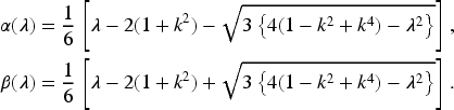
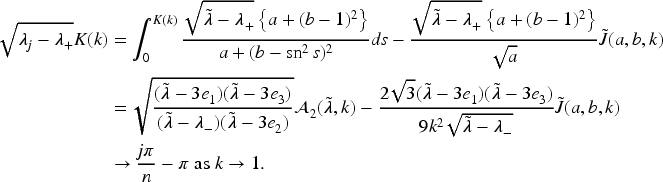
(ii) Let us consider the first case. Let $j \in {1, 2, \dots, n - 1}$ be fixed. Let $\tilde{λ} = λ_{2 j - 1}^{(n)} = λ_{2 j}^{(n)}$ . We consider the equation

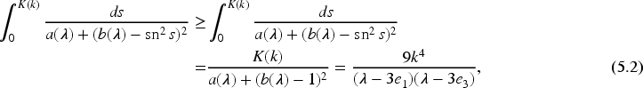
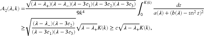
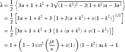
\begin{aligned} A_{2} (λ, k) = \frac{j π}{n} . \end{aligned}

(5.3)

Lemmas 5.1 and 5.2 indicate that a solution

\tilde{λ}

of (5.3) is unique and

λ_{-} < \tilde{λ} < 3 e_{3}

. Since

\begin{aligned} - 2 \sqrt{1 - k^{2} + k^{4}} < \tilde{λ} < - 1 - k^{2}, \end{aligned}

(5.4)

we have

\begin{aligned} 3 < \frac{- \tilde{λ} - 2 + 4 k^{2}}{1 - k^{2}} < \frac{2}{1 - k^{2}} (\sqrt{1 - k^{2} + k^{4}} + 1 - 2 k^{2}) = \frac{6 k^{2}}{\sqrt{1 - k^{2} + k^{4}} - 1 + 2 k^{2}} \to 3 as k \to 1. \end{aligned}

Thus,

\begin{aligned} \frac{- \tilde{λ} - 2 + 4 k^{2}}{1 - k^{2}} \to 3 as k \to 1. \end{aligned}

By (5.4) we have

\begin{aligned} 0 < \frac{\sqrt{4 (1 - k^{2} + k^{4}) - {\tilde{λ}}^{2}}}{\sqrt{3} (1 - k^{2})} < 1. \end{aligned}

(5.5)

Letting

k \to 1

, we have a convergent subsequence of

\tilde{λ}

which is still denoted by

\tilde{λ}

. Then there exists

λ^{*} \in [0, 1]

such that

\begin{aligned} \frac{\sqrt{4 (1 - k^{2} + k^{4}) - {\tilde{λ}}^{2}}}{\sqrt{3} (1 - k^{2})} \to \sqrt{λ^{*}} as k \to 1. \end{aligned}

Then, by (5.4) and (5.5) we have

\begin{aligned} \frac{- α (\tilde{λ}) - k^{2}}{1 - k^{2}} & = \frac{1}{6} \frac{- \tilde{λ} - 2 + 4 k^{2}}{1 - k^{2}} + \frac{1}{2} \frac{\sqrt{4 (1 - k^{2} + k^{4}) - {\tilde{λ}}^{2}}}{\sqrt{3} (1 - k^{2})} \to \frac{1 + \sqrt{λ^{*}}}{2} as k \to 1, \end{aligned}

(5.6)

\begin{aligned} \frac{- β (\tilde{λ}) - k^{2}}{1 - k^{2}} & = \frac{1}{6} \frac{- \tilde{λ} - 2 + 4 k^{2}}{1 - k^{2}} - \frac{1}{2} \frac{\sqrt{4 (1 - k^{2} + k^{4}) - {\tilde{λ}}^{2}}}{\sqrt{3} (1 - k^{2})} \to \frac{1 - \sqrt{λ^{*}}}{2} as k \to 1. \end{aligned}

By Lemma 7.4 we see that, as

k \to 1

\begin{aligned} (\frac{j π}{n} =) A_{2} (\tilde{λ}, k) & \to | - \frac{π}{2} + \tan^{- 1} \sqrt{\frac{1 - \sqrt{λ^{*}}}{1 + \sqrt{λ^{*}}}} - (- \frac{π}{2} + \tan^{- 1} \sqrt{\frac{1 + \sqrt{λ^{*}}}{1 - \sqrt{λ^{*}}}}) | \\ = | - \tan^{- 1} \sqrt{\frac{1 + \sqrt{λ^{*}}}{1 - \sqrt{λ^{*}}}} - (- \frac{π}{2} + \tan^{- 1} \sqrt{\frac{1 + \sqrt{λ^{*}}}{1 - \sqrt{λ^{*}}}}) | = 2 \tan^{- 1} \sqrt{\frac{1 + \sqrt{λ^{*}}}{1 - \sqrt{λ^{*}}}} - \frac{π}{2} . \end{aligned}

Solving

\begin{aligned} \frac{j π}{n} = 2 \tan^{- 1} \sqrt{\frac{1 + \sqrt{λ^{*}}}{1 - \sqrt{λ^{*}}}} - \frac{π}{2} \end{aligned}

with respect to

λ^{*}

, we have

\begin{aligned} λ^{*} = \sin^{2} (\frac{j π}{n}) . \end{aligned}

Using (5.6), we have

\begin{aligned} α (\tilde{λ}) + k^{2} = - \frac{1}{2} (\sin (\frac{j π}{n}) + 1) (1 - k^{2}) + o (1 - k^{2}) . \end{aligned}

(5.7)

Since

λ_{-} < \tilde{λ} < 3 e_{1}

\tilde{λ}

is the smaller root of

\begin{aligned} λ^{2} - (3 α + 1 + k^{2}) λ + 9 α^{2} + 6 (1 + k^{2}) α - 2 + 5 k^{2} - 2 k^{4} = 0. \end{aligned}

Note that the larger root is in

(3 e_{2}, 3 e_{1})

. By (5.7) we have

\begin{aligned} \tilde{λ} & = \frac{1}{2} {3 α + 1 + k^{2} - 3 \sqrt{(1 - k^{2})^{2} - 2 (1 + k^{2}) α - 3 α^{2}}} \\ = \frac{1}{2} [3 α + 1 + k^{2} - 3 {1 + 2 (α + k^{2}) - 3 (α + k^{2})^{2} - 4 (α + k^{2}) (1 - k^{2})}^{1 / 2}] \\ = \frac{1}{2} [3 α + 1 + k^{2} - 3 {1 + \frac{1}{2} {2 (α + k^{2}) - 3 (α + k^{2})^{2} - 4 (α + k^{2}) (1 - k^{2})} \\ - \frac{4}{8} (α + k^{2})^{2} + o ((1 - k^{2})^{2})}] \\ = - 2 + (1 - k^{2}) + \frac{3}{4} (\sin^{2} (\frac{j π}{n}) - 1) (1 - k^{2})^{2} + o ((1 - k^{2})^{2}) as k \to 1. \end{aligned}

Next, we consider the second case. Let $j \in {n + 1, n + 2, \dots, 2 n - 1}$ be fixed. Let $\tilde{λ} = λ_{2 j - 1}^{(n)} = λ_{2 j}^{(n)}$ for simplicity. We consider (5.3). Lemmas 5.1 and 5.2 indicate that a solution $\tilde{λ}$ of (5.3) is unique and $3 e_{2} < \tilde{λ} < 3 e_{1}$ . By elementary argument we see that $- 1 < α (\tilde{λ}) < - k^{2}$ . Therefore,

\begin{aligned} 0 < \frac{- α (\tilde{λ}) - k^{2}}{1 - k^{2}} < 1. \end{aligned}

Letting

k \to 1

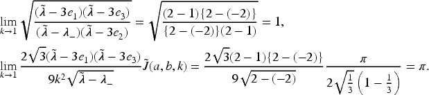
, we have a convergent subsequence of

\tilde{λ}

which is denoted by

\tilde{λ}

. Then,

\begin{aligned} there exists α^{*} \in [0, 1] such that lim_{k \to 1} \frac{- α (\tilde{λ}) - k^{2}}{1 - k^{2}} = α^{*} . \end{aligned}

(5.8)

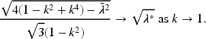
By Lemma 7.4 we have

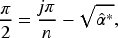
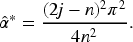
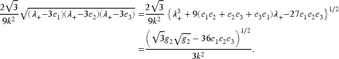
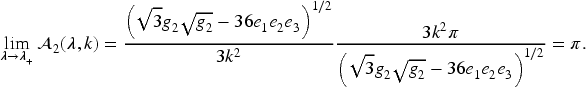
\begin{aligned} M (α (\tilde{λ}), k) \to - (\frac{π}{2} - \tan^{- 1} \sqrt{\frac{α^{*}}{1 - α^{*}}}) as k \to 1. \end{aligned}

(5.9)

On the other hand, by elementary argument we see that

β (3 e_{2}) = β (3 e_{1})

β (λ) > 0

for

3 e_{3} < λ < 3 e_{1}

and

β (λ)

has a unique maximum point

\hat{λ}

3 e_{2} < λ < 3 e_{1}

which satisfies

\sqrt{3 {4 (1 - k^{2} + k^{4}) - {\hat{λ}}^{2}}} = 3 \hat{λ}

. Hence,

\begin{aligned} 0 \leq β (\tilde{λ}) \leq β (\hat{λ}) = \frac{1}{6} {\hat{λ} - 2 (1 + k^{2}) + 3 \hat{λ}} \leq \frac{1}{6} {12 e_{1} - 2 (1 + k^{2})} = 1 - k^{2} . \end{aligned}

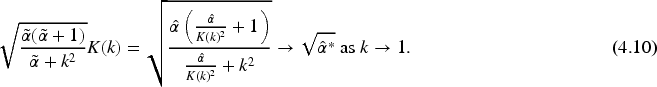
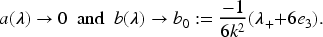
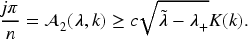
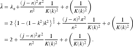
In particular,

β (\tilde{λ}) \to 0

k \to 1

. Using Lemma 7.1, we have

\begin{aligned} 0 \leq \sqrt{β (\tilde{λ})} K (k) \leq \sqrt{1 - k^{2}} K (k) = \sqrt{1 - k^{2}} (\log \frac{1}{\sqrt{1 - k^{2}}} + 2 \log 2 + o (1)) \to 0 as k \to 1. \end{aligned}

(5.10)

Let

J (ν, k)

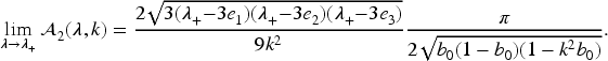
be defined by (7.5). By Lemma 7.3 and (5.10) we have

\begin{aligned} M (β (\tilde{λ}), k) = \sqrt{β (\tilde{λ}) + 1} J (\frac{k^{2}}{β (\tilde{λ}), k}) + \sqrt{\frac{β (\tilde{λ}) (β (\tilde{λ}) + 1)}{β (\tilde{λ}) + k^{2}}} K (k) \to \frac{π}{2} as k \to 1. \end{aligned}

(5.11)

Thus, by (5.9) and (5.11) we see that, as

k \to 1

\begin{aligned} (\frac{j π}{n} =) A_{2} (\tilde{λ}, k) = & | M (β (\tilde{λ}), k) - M (α (\tilde{λ}), k) | \\ \to & | \frac{π}{2} + (\frac{π}{2} - \tan^{- 1} \sqrt{\frac{α^{*}}{1 - α^{*}}}) | = π - \tan^{- 1} \sqrt{\frac{α^{*}}{1 - α^{*}}} . \end{aligned}

Solving

\begin{aligned} \frac{j π}{n} = π - \tan^{- 1} \sqrt{\frac{α^{*}}{1 - α^{*}}} \end{aligned}

with respect to

α^{*}

, we have

\begin{aligned} α^{*} = \sin^{2} (\frac{j π}{n}) . \end{aligned}

By (5.8) we have

\begin{aligned} α (\tilde{λ}) + k^{2} = - (\sin^{2} (\frac{j π}{n}) + o (1)) (1 - k^{2}) as k \to 1. \end{aligned}

(5.12)

Since

3 e_{2} < \tilde{λ} < 3 e_{1}

\tilde{λ}

is the larger root of

\begin{aligned} λ - (3 α + 1 + k^{2}) λ + 9 α^{2} + 6 (1 + k^{2}) α - 2 + 5 k^{2} - 2 k^{4} = 0. \end{aligned}

Note that the smaller root is in

(λ_{-}, 3 e_{3})

. Using (5.12), we have

\begin{aligned} \tilde{λ} & = \frac{1}{2} {3 α + 1 + k^{2} + 3 \sqrt{(1 - k^{2})^{2} - 2 (1 + k^{2}) α - 3 α^{2}}} \\ = \frac{1}{2} [3 α + 1 + k^{2} + 3 {1 + 2 (α + k^{2}) + o (1 - k^{2})}^{1 / 2}] \\ = \frac{1}{2} [3 α + 1 + k^{2} + 3 {1 + (α + k^{2}) + o (1 - k^{2})}] \\ = 1 + (1 - 3 \sin^{2} (\frac{j π}{n}) + o (1)) (1 - k^{2}) as k \to 1. \end{aligned}

We consider the third case. Let $j \in {2 n + 1, 2 n + 2, \dots}$ . Let $\tilde{λ} = λ_{2 j - 1}^{(n)} = λ_{2 j}^{(n)}$ for simplicity. We have

\begin{aligned} \frac{j π}{n} = A_{2} (λ, k) \geq c \sqrt{\tilde{λ} - λ_{+}} K (k) . \end{aligned}

This implies that

lim_{k \to 1} (\tilde{λ} - λ_{+}) = 0

, and hence

\begin{aligned} lim_{k \to 1} \tilde{λ} = 2. \end{aligned}

(5.13)

Let

\begin{aligned} a (λ) := \frac{1}{12 k^{4}} {λ^{2} - 4 (1 - k^{2} + k^{4})} and b (λ) := \frac{1}{6 k^{2}} (2 + 2 k^{2} - λ) . \end{aligned}

Then,

\begin{aligned} lim_{k \to 1} a (λ_{j}) = 0 and b_{0} := lim_{k \to 1} b (λ_{j}) = \frac{1}{3} . \end{aligned}

Moreover,

\begin{aligned} A_{2} (λ, k) = \frac{2 \sqrt{3 a (λ - 3 e_{1}) (λ - 3 e_{2}) (λ - 3 e_{3})}}{9 k^{2}} \int_{0}^{K (k)} \frac{d s}{a + (b - {sn}^{2} s)^{2}} . \end{aligned}

Using (5.13),

\begin{aligned} \sqrt{a (λ)} = \frac{1}{2 \sqrt{3} k^{2}} \sqrt{(λ - λ_{+}) (λ - λ_{-})} and a (λ) + (b (λ) - 1)^{2} = \frac{1}{9 k^{4}} (λ - 3 e_{1}) (λ - 3 e_{3}), \end{aligned}

by Lemma 7.6 we have

\begin{aligned} \sqrt{λ_{j} - λ_{+}} K (k) & = \int_{0}^{K (k)} \frac{\sqrt{\tilde{λ} - λ_{+}} {a + (b - 1)^{2}}}{a + (b - {sn}^{2} s)^{2}} d s - \frac{\sqrt{\tilde{λ} - λ_{+}} {a + (b - 1)^{2}}}{\sqrt{a}} \tilde{J} (a, b, k) \\ = \sqrt{\frac{(\tilde{λ} - 3 e_{1}) (\tilde{λ} - 3 e_{3})}{(\tilde{λ} - λ_{-}) (\tilde{λ} - 3 e_{2})}} A_{2} (\tilde{λ}, k) - \frac{2 \sqrt{3} (\tilde{λ} - 3 e_{1}) (\tilde{λ} - 3 e_{3})}{9 k^{2} \sqrt{\tilde{λ} - λ_{-}}} \tilde{J} (a, b, k) \\ \to \frac{j π}{n} - π as k \to 1. \end{aligned}

Here we used

\begin{aligned} lim_{k \to 1} \sqrt{\frac{(\tilde{λ} - 3 e_{1}) (\tilde{λ} - 3 e_{3})}{(\tilde{λ} - λ_{-}) (\tilde{λ} - 3 e_{2})}} = \sqrt{\frac{(2 - 1) {2 - (- 2)}}{{2 - (- 2)} (2 - 1)}} = 1, \\ lim_{k \to 1} \frac{2 \sqrt{3} (\tilde{λ} - 3 e_{1}) (\tilde{λ} - 3 e_{3})}{9 k^{2} \sqrt{\tilde{λ} - λ_{-}}} \tilde{J} (a, b, k) = \frac{2 \sqrt{3} (2 - 1) {2 - (- 2)}}{9 \sqrt{2 - (- 2)}} \frac{π}{2 \sqrt{\frac{1}{3}} (1 - \frac{1}{3})} = π . \end{aligned}

Lemma 7.1 indicates that

(1 - k^{2}) K {(k)}^{2} \to 0

k \to 1

, and hence

\begin{aligned} 1 - k^{2} = o (\frac{1}{K {(k)}^{2}}) . \end{aligned}

(5.14)

Using (5.14), we have

\begin{aligned} \tilde{λ} & = λ_{+} + \frac{(j - n)^{2} π^{2}}{n^{2}} \frac{1}{K {(k)}^{2}} + o (\frac{1}{K {(k)}^{2}}) \\ = 2 {1 - (1 - k^{2}) k^{2}}^{\frac{1}{2}} + \frac{(j - n)^{2} π^{2}}{n^{2}} \frac{1}{K {(k)}^{2}} + o (\frac{1}{K {(k)}^{2}}) \\ = 2 + \frac{(j - n)^{2} π^{2}}{n^{2}} \frac{1}{K {(k)}^{2}} + o (\frac{1}{K {(k)}^{2}}) . \end{aligned}

The set

{λ_{j}^{(n)}}_{j = 0}^{\infty}

consist of all the eigenvalues, since we have examined all

λ \in closure (σ_{2})

in proofs of Theorem 1.3 (i) and (ii). Every eigenvalue in Theorem 1.3 (ii) has multiplicity

2

, since

ϕ^{e}

and

ϕ^{o}

are solutions of (5.1). The proof is complete.

6. Applications

In this section let $u (y)$ denote an unknown function of nonlinear problems, and let $μ_{j}^{(m)}$ denote an eigenvalue for a linearization around an $m$ -mode solution $u_{m} (y)$ . Moreover, in the case of a periodic or Neumann boundary condition $j$ starts from $0$ , i.e., the first eigenvalue is $μ_{0}^{(m)}$ . However in the case of a Dirichlet boundary condition $j$ starts from $1$ , i.e., the first eigenvalue is $μ_{1}^{(m)}$ .

6.1. Allen–Cahn Equation

(1) We consider the nonlinear problem with periodic boundary condition:

\begin{aligned} ε^{2} u^{″} + u - u^{3} = 0 for y \in R / Z . \end{aligned}

All nontrivial solutions can be expressed as

\begin{aligned} ε_{m} = \frac{1}{4 m \sqrt{1 + k^{2}} K (k)} and u_{m}^{\pm} (y) = \pm \sqrt{\frac{2 k^{2}}{1 + k^{2}}} sn (4 m K (k) y + y_{0}, k) \end{aligned}

for

y_{0} \in R

m = 1, 2, \dots

and

0 < k < 1

. We consider the solutions with

y_{0} = 0

. The linearized eigenvalue problem becomes

\begin{aligned} ε^{2} ψ^{″} + {1 - {(u_{m}^{\pm})}^{2}} ψ = - μ ψ for y \in R / Z . \end{aligned}

Since

1 - (u_{m}^{+})^{2} = 1 - (u_{m}^{-})^{2}

, an eigenvalue for

u_{m}^{+}

is equal to that for

u_{m}^{-}

, and hence

μ_{j}^{(m)}

denotes the eigenvalue for both

u_{m}^{+}

and

u_{m}^{-}

. Then, the linearization problem around

u_{m}^{\pm}

\begin{aligned} - \frac{1}{16 m^{2} (1 + k^{2}) K {(k)}^{2}} ψ^{″} + {- 1 + \frac{6 k^{2}}{1 + k^{2}} {sn}^{2} (4 m K (k) y, k)} ψ = μ ψ for y \in R / Z . \end{aligned}

Let

x := 4 m K (k) y

and

ϕ (x) := ψ (y)

. Then,

\begin{aligned} - ϕ^{″} + {- 2 - 2 k^{2} + 6 k^{2} {sn}^{2} (x, k)} ϕ = (1 + k^{2}) (μ - 1) ϕ for x \in R / 4 m K (k) Z . \end{aligned}

(6.1)

The problem (6.1) is equivalent to (1.4) with

n = 2 m

. Thus,

(1 + k^{2}) (μ_{j}^{(m)} - 1) = λ_{j}^{(2 m)}

for

j = 0, 1, 2, \dots

, and hence

\begin{aligned} μ_{j}^{(m)} = \frac{1}{1 + k^{2}} λ_{j}^{(2 m)} + 1 for j = 0, 1, 2, \dots . \end{aligned}

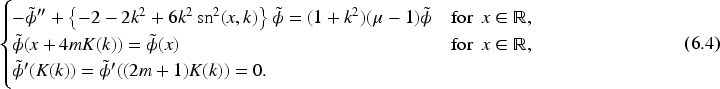
(2) We consider the Dirichlet problem

\begin{aligned} {\begin{cases} ε^{2} u^{″} + u - u^{3} = 0 & for 0 < y < 1, \\ u (0) = u (1) = 0. \end{cases} \end{aligned}

Then, all nontrivial solutions can be expressed as

\begin{aligned} ε_{m} = \frac{1}{2 m \sqrt{1 + k^{2}} K (k)} and u_{m}^{\pm} (y) = \pm \sqrt{\frac{2 k^{2}}{1 + k^{2}}} sn (2 m K (k) y, k) \end{aligned}

for

m = 1, 2, \dots

and

0 < k < 1

. The linearization problem around

u_{m}^{\pm}

\begin{aligned} {\begin{cases} - \frac{1}{4 m^{2} (1 + k^{2}) K {(k)}^{2}} ψ^{″} + {- 1 + \frac{6 k^{2}}{1 + k^{2}} {sn}^{2} (2 m K (k) y, k)} ψ = μ ψ for 0 < y < 1, \\ ψ (0) = ψ (1) = 0. \end{cases} \end{aligned}

Let

x := 2 m (K) y

and

ϕ (x) = ψ (y)

. Then,

\begin{aligned} {\begin{cases} - ϕ^{″} + {- 2 - 2 k^{2} + 6 k^{2} {sn}^{2} (x, k)} ϕ = (1 + k^{2}) (μ - 1) ϕ for 0 < x < 2 m K (k), \\ ϕ (0) = ϕ (2 m K (k)) = 0. \end{cases} \end{aligned}

By odd reflection we extend

ϕ (x)

\tilde{ϕ} (x)

defined on

R

. Then,

\tilde{ϕ} (x)

satisfies

\begin{aligned} {\begin{cases} - {\tilde{ϕ}}^{″} + {- 2 - 2 k^{2} + 6 k^{2} {sn}^{2} (x, k)} \tilde{ϕ} = (1 + k^{2}) (μ - 1) \tilde{ϕ} & for x \in R, \\ \tilde{ϕ} (x + 4 m K (k)) = \tilde{ϕ} (x) & for x \in R, \\ \tilde{ϕ} (0) = \tilde{ϕ} (2 m K (k)) = 0. \end{cases} \end{aligned}

(6.2)

We choose all eigenfunctions of (1.4) with

n = 2 m

that satisfy (6.2). Since

n (= 2 m)

is even, in Theorem 1.3 (i) only

ϕ_{n} (x)

and

ϕ_{2 n - 1} (x)

satisfy (6.2). In Theorem 1.3 (ii) every eigenvalue has multiplicity

2

, i.e.,

λ_{j - 1}^{(2 m)} = λ_{j}^{(2 m)}

for

j \in 2 N ∖ {2 m, 4 m}

. An eigenfunction

ϕ^{o} (x)

associated with

λ_{j}^{(2 m)}

j \in 2 N ∖ {2 m, 4 m}

, satisfies (6.2). Thus, we obtain

\begin{aligned} μ_{j}^{(m)} = {\begin{cases} 1 + λ_{2 j}^{(2 m)} / (1 + k^{2}) & for j \in {1, 2, \dots, m - 1}, & (by (ii)) \\ 1 + λ_{2 m - 1}^{(2 m)} / (1 + k^{2}) = 3 k^{2} / (1 + k^{2}) & for j = m, & (by (i)) \\ 1 + λ_{2 j}^{(2 m)} / (1 + k^{2}) & for j \in {m + 1, \dots, 2 m - 1}, & (by (ii)) \\ 1 + λ_{4 m - 1}^{(2 m)} / (1 + k^{2}) = 3 / (1 + k^{2}) & for j = 2 m, & (by (i)) \\ 1 + λ_{2 j}^{(2 m)} / (1 + k^{2}) & for j \in {2 m + 1, 2 m + 2, \dots} . & (by (ii)) \end{cases} \end{aligned}

It is equivalent to the following:

\begin{aligned} μ_{j}^{(m)} = 1 + \frac{λ_{2 j}^{(2 m)}}{1 + k^{2}} for j \in N ∖ {2 m}, μ_{2 m}^{(m)} = 1 + \frac{λ_{4 m - 1}^{(2 m)}}{1 + k^{2}} . \end{aligned}

(3) We consider the Neumann problem

\begin{aligned} {\begin{cases} ε^{2} u^{″} + u - u^{3} = 0 & for 0 < y < 1, \\ u^{'} (0) = u^{'} (1) = 0. \end{cases} \end{aligned}

(6.3)

All nontrivial solutions can be expressed by

\begin{aligned} ε_{m} := \frac{1}{2 m \sqrt{1 + k^{2}} K (k)} and u_{m}^{\pm} (y) := \pm \sqrt{\frac{2 k^{2}}{1 + k^{2}}} sn ((2 m y + 1) K (k), k) \end{aligned}

for

m = 1, 2, \dots

and

0 < k < 1

. The linearization problem around

u_{m}^{\pm}

\begin{aligned} {\begin{cases} - \frac{1}{4 m^{2} (1 + k^{2}) K {(k)}^{2}} ψ^{″} + {- 1 + \frac{6 k^{2}}{1 + k^{2}} {sn}^{2} ((2 m y + 1) K (k), k)} ψ = μ ψ & for 0 < y < 1, \\ ψ^{'} (0) = ψ^{'} (2 m K (k)) = 0. \end{cases} \end{aligned}

Let

x := (2 m y + 1) K (k)

and

ϕ (x) := ψ (y)

. Then,

\begin{aligned} {\begin{cases} - ϕ^{″} + {- 2 - 2 k^{2} + 6 k^{2} {sn}^{2} (x, k)} ϕ = (1 + k^{2}) (μ - 1) ϕ & for K (k) < x < (2 m + 1) K (k), \\ ϕ^{'} (K (k)) = ϕ^{'} ((2 m + 1) K (k)) = 0. \end{cases} \end{aligned}

By even reflection we extend

ϕ (x)

\tilde{ϕ} (x)

defined on

R

. Then,

\tilde{ϕ} (x)

satisfies

\begin{aligned} {\begin{cases} - {\tilde{ϕ}}^{″} + {- 2 - 2 k^{2} + 6 k^{2} {sn}^{2} (x, k)} \tilde{ϕ} = (1 + k^{2}) (μ - 1) \tilde{ϕ} & for x \in R, \\ \tilde{ϕ} (x + 4 m K (k)) = \tilde{ϕ} (x) & for x \in R, \\ {\tilde{ϕ}}^{'} (K (k)) = {\tilde{ϕ}}^{'} ((2 m + 1) K (k)) = 0. \end{cases} \end{aligned}

(6.4)

We choose all eigenfunctions of (1.4) with

n = 2 m

that satisfies (6.4). Since

n (= 2 m)

is even, in Theorem 1.3 (i) only

ϕ_{0} (x)

ϕ_{n} (x)

and

ϕ_{2 n} (x)

satisfy (6.4). In Theorem 1.3 (ii) every eigenvalue has multiplicity

2

. An eigenfunction

\begin{aligned} (\cos x_{0}) ϕ^{e} (x) + (\sin x_{0}) ϕ^{o} (x) = \sqrt{| {\tilde{Ξ}}_{2} (x, λ) |} \cos (\int_{0}^{x} \frac{\sqrt{Q_{2} (λ)}}{| {\tilde{Ξ}}_{2} (s, λ) |} d s - \int_{0}^{K (k)} \frac{\sqrt{Q_{2} (λ)}}{| {\tilde{Ξ}}_{2} (s, λ) |} d s) \end{aligned}

associated with

λ_{j}^{(2 m)}

j \in 2 N ∖ {2 m, 4 m}

, satisfies (6.4), where

x_{0} := \int_{0}^{K (k)} \frac{\sqrt{Q_{2} (λ)}}{| {\tilde{Ξ}}_{2} (s, λ) |} d s

. Since

{0, 2 m, 4 m} \cup (2 N ∖ {2 m, 4 m}) = {0, 2, 4, 6, \dots}

, we obtain

\begin{aligned} μ_{j}^{(m)} = \frac{λ_{2 j}^{(2 m)}}{1 + k^{2}} + 1 for j \in {0, 1, 2, \dots} . \end{aligned}

6.2. Scalar Field Equation

(4) In this subsection we consider only periodic boundary value problem

\begin{aligned} ε^{2} u^{″} - u + u^{3} = 0 for y \in R / Z . \end{aligned}

(6.5)

Dirichlet and Neumann problems can be treated in the same way as in Subsection 6.1. All sign-changing solutions of (6.5) can be expressed by

\begin{aligned} ε_{m} := \frac{1}{4 m \sqrt{2 k^{2} - 1} K (k)} and u_{m}^{(c, \pm)} (y) := \pm \sqrt{\frac{2 k^{2}}{2 k^{2} - 1}} cn (4 m K (k) y + y_{0}, k) \end{aligned}

for

y_{0} \in R

m = 1, 2, \dots

and

1 / \sqrt{2} < k < 1

. We consider the case

y_{0} = 0

. Using the same method as the problem (6.3), we obtain

\begin{aligned} - ϕ^{″} + {- 2 - 2 k^{2} + 6 k^{2} {sn}^{2} (x, k)} ϕ = (2 k^{2} - 1) (μ + 1) ϕ for x \in R / 4 m K (k) Z . \end{aligned}

Comparing this problem with (1.4), we obtain the following relation:

\begin{aligned} μ_{j}^{(m)} = \frac{λ_{j}^{(2 m)}}{2 k^{2} - 1} - 1 for j = 0, 1, 2, \dots . \end{aligned}

(5) The problem (6.5) has the following positive and negative solutions:

\begin{aligned} ε_{m} := \frac{1}{2 m \sqrt{2 - k^{2}} K (k)} and u_{m}^{(d, \pm)} (y) := \pm \sqrt{\frac{2}{2 - k^{2}}} dn (2 m K (k) y + y_{0}, k) \end{aligned}

for

y_{0} \in R

m = 1, 2, \dots

and

0 < k < 1

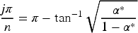
. See Miyamoto et al. (2023) for details. We also consider the case

y_{0} = 0

. Then, we have

\begin{aligned} - ϕ^{″} + {- 2 - 2 k^{2} + 6 k^{2} {sn}^{2} (x, k)} ϕ = (2 - k^{2}) (μ + 1) ϕ for x \in R / 2 m K (k) Z . \end{aligned}

In this case the following relation holds:

\begin{aligned} μ_{j}^{(m)} = \frac{λ_{j}^{(m)}}{2 - k^{2}} - 1 for j = 0, 1, 2, \dots . \end{aligned}

6.3. sine-Poisson Equation and Other Equations

(6) We consider the sine-Poisson equation

\begin{aligned} ε^{2} u^{″} + \sin u = 0 for y \in R / Z . \end{aligned}

This problem has nontrivial solutions

\begin{aligned} ε_{m} := \frac{1}{4 m K (k)} and u_{m}^{\pm} (y) := \pm 2 \sin^{- 1} (k sn (4 m K (k) y + y_{0}, k)) . \end{aligned}

for

y_{0} \in R

m = 1, 2, \dots

and

0 < k < 1

. See Wakasa and Yotsutani (2008) for details. We consider the case

y_{0} = 0

. Let

x := 4 m K (k) y

. Then the linearized eigenvalue problem can be transformed into

\begin{aligned} - ϕ^{″} + {- 1 - k^{2} + 2 k^{2} {sn}^{2} (x, k)} ϕ = (μ - k^{2}) ϕ for x \in R / 4 m K (k) Z . \end{aligned}

Thus, an eigenvalue

μ_{j}^{(m)}

can be related to the eigenvalue

α_{j}^{(2 m)}

of (1.2) with

n = 2 m

. Specifically, we have

\begin{aligned} μ_{j}^{(m)} = α_{j}^{(2 m)} + k^{2} for j = 0, 1, 2, \dots . \end{aligned}

(7) Details of this case are omitted. The eigenvalue relation is given by (1.21).

(8) We consider the sinh-Poisson equation

\begin{aligned} ε^{2} u^{″} + \sinh u = 0 for y \in R / Z . \end{aligned}

All solutions can be expressed by

\begin{aligned} ε_{m} & := \frac{1}{4 m \sqrt{1 - k^{2}} K (k)} and \\ u_{m}^{\pm} (y) & := \pm [2 \log {dn (4 m K (k) y + y_{0}, k) + k cn (4 m K (k) y + y_{0}, k)} - \log (1 - k^{2})] . \end{aligned}

Details can be found in Aizawa et al. (2023). We consider the case

y_{0} = 0

. Let

x := 4 m K (k) y

. Then the linearized eigenvalue problem can be transformed into

\begin{aligned} - ϕ^{″} + {- 1 - k^{2} + 2 k^{2} {sn}^{2} (x, k)} ϕ = (1 - k^{2}) μ ϕ for x \in R / 4 m K (k) Z . \end{aligned}

Therefore,

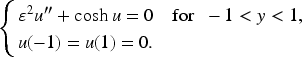
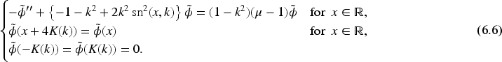
\begin{aligned} μ_{j}^{(m)} = \frac{α_{j}^{(2 m)}}{1 - k^{2}} for j = 0, 1, 2, \dots . \end{aligned}

(9) We consider the Dirichlet problem

\begin{aligned} {\begin{cases} ε^{2} u^{″} + \cosh u = 0 & for - 1 < y < 1, \\ u (- 1) = u (1) = 0. \end{cases} \end{aligned}

All solutions can be expressed as

\begin{aligned} ε_{m} := \frac{1}{\sqrt{1 - k^{2}} K (k)} and u (x) := 2 \sinh^{- 1} (\sqrt{\frac{k^{2}}{1 - k^{2}}} cn (K (k) y, k)) \end{aligned}

for

0 < k < 1

. Let

x := K (k) y

. The linearization problem becomes

\begin{aligned} {\begin{cases} - ϕ^{″} + {- 1 - k^{2} + 2 k^{2} {sn}^{2} (x, k)} ϕ = (1 - k^{2}) (μ - 1) ϕ & for - K (k) < x < K (k), \\ ϕ (- K (k)) = ϕ (K (k)) = 0. \end{cases} \end{aligned}

By odd reflection we extend

ϕ (x)

\tilde{ϕ} (x)

defined on

R

. Then

\tilde{ϕ}

satisfies

\begin{aligned} {\begin{cases} - {\tilde{ϕ}}^{″} + {- 1 - k^{2} + 2 k^{2} {sn}^{2} (x, k)} \tilde{ϕ} = (1 - k^{2}) (μ - 1) \tilde{ϕ} & for x \in R, \\ \tilde{ϕ} (x + 4 K (k)) = \tilde{ϕ} (x) & for x \in R, \\ \tilde{ϕ} (- K (k)) = \tilde{ϕ} (K (k)) = 0. \end{cases} \end{aligned}

(6.6)

Since

\tilde{ϕ}

4 K (k)

-periodic, we set

n = 2

. In Theorem 1.1 (i) only

ϕ_{n - 1} (x)

satisfies (6.6). Every eigenfunction in Theorem 1.1 (ii) has multiplicity

2

, i.e.,

α_{j - 1}^{(2)} = α_{j}^{(2)}

for

j \in 2 N ∖ {2}

. An eigenfunction

(\cos x_{0}) ϕ^{e} (x) + (\sin x_{0}) ϕ^{o} (x)

associated with

α_{j}^{(2)}

j \in {3, 5, 7, \dots}

, satisfies (6.6), where

x_{0} = \int_{0}^{K (k)} \frac{\sqrt{Q_{1} (λ)}}{{\tilde{Ξ}}_{1} (y, λ)} d y

. Since

{1} \cup {3, 5, 7, \dots} = {1, 3, 5, \dots}

, we obtain

\begin{aligned} μ_{j} = \frac{α_{j}^{(2)}}{1 - k^{2}} + 1 for j = 1, 3, 5, \dots . \end{aligned}

6.4. 1D Gel’fand Problem

We consider the Dirichlet problem

\begin{aligned} {\begin{cases} ε^{2} u^{″} + e^{u} = 0 & for - 1 < y < 1, \\ u (- 1) = u (1) = 0. \end{cases} \end{aligned}

Then, all solutions can be written as follows:

\begin{aligned} ε := \frac{\cosh τ}{\sqrt{2} τ} and u (y) := 2 \log \frac{\cosh τ}{\cosh τ y} \end{aligned}

for

τ > 0

. Let

x := τ y

. The linearization problem can be transformed into the following:

\begin{aligned} {\begin{cases} - η^{″} - 2 ({sech}^{2} x) η = 2 μ ({sech}^{2} τ) η & for - τ < x < τ, \\ η (- τ) = η (τ) = 0, \end{cases} \end{aligned}

(6.7)

where

η (x)

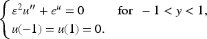
is an unknown function. We consider the following ODE

\begin{aligned} - ϕ^{″} - 2 ({sech}^{2} x) ϕ = α ϕ for x \in R, \end{aligned}

(6.8)

where

ϕ (x)

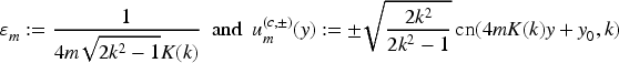
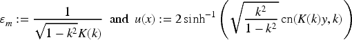
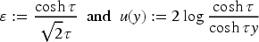
is an unknown function. The equation (6.8) has the Pöschl–Teller potential

- ℓ (ℓ + 1) {sech}^{2} x

with

ℓ = 1

for which all eigenvalues of

- ϕ^{″} - ℓ (ℓ + 1) ({sech}^{2} x) ϕ = α ϕ

L^{2} (R)

can be obtained explicitly, i.e., the eigenvalues are

{- 1, - 4, - 9, \dots, - ℓ^{2}}

. It is known that the spectral set of (6.8) is

{- 1} \cup [0, \infty)

, where

[0, \infty)

is a continuous spectrum. Bounded solutions of the ODE in (6.8) are given by

\begin{aligned} {\begin{aligned} ϕ^{+, e} (x) & = \sqrt{α + \tanh^{2} x} \cos (\sqrt{α} x + \tan^{- 1} (\frac{\tanh x}{\sqrt{α}})) \\ ϕ^{+, o} (x) & = \sqrt{α + \tanh^{2} x} \sin (\sqrt{α} x + \tan^{- 1} (\frac{\tanh x}{\sqrt{α}})) \end{aligned} for α > 0, \\ ϕ^{0, o} (x) = \tanh x for α = 0, \\ ϕ^{- 1, e} (x) = sech x for α = - 1. \end{aligned}

Therefore, putting

α = 2 μ {sech}^{2} τ

and finding all solutions satisfying

ϕ (\pm τ) = 0

, we obtain all eigenvalues

μ_{j}

. Details can be found in Miyamoto and Wakasa (2019).

Now, let us study a relation between (6.8) and (4.1) on $X_{k}^{(2)}$ . It is known that

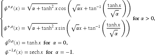
\begin{aligned} sn (x, k) \to \tanh x uniformly for x in any compact interval as k \to 1 . \end{aligned}

Therefore, roughly speaking, (4.1) converges to (6.8) as

k \to 1

. We show that a solution of (4.1) converges to that of (6.8) as

k \to 1

. When

α > 0

, two independent solutions of (4.1) are given by (4.2), i.e.,

\begin{aligned} {\begin{cases} ϕ_{k}^{+, e} (x) = \sqrt{| α + k^{2} {sn}^{2} x |} \cos (\int_{0}^{x} \frac{\sqrt{α (α + 1) (α + k^{2})} d s}{α + k^{2} {sn}^{2} s}), \\ ϕ_{k}^{+, o} (x) = \sqrt{| α + k^{2} {sn}^{2} x |} \sin (\int_{0}^{x} \frac{\sqrt{α (α + 1) (α + k^{2})} d s}{α + k^{2} {sn}^{2} s}) . \end{cases} \end{aligned}

By the dominated convergence theorem we see that, as

k \to 1

\begin{aligned} ϕ_{k}^{+, e} (x) \to ϕ^{+, e} (x) and ϕ_{k}^{+, o} (x) \to ϕ^{+, o} (x), \end{aligned}

because of the integral formula

\begin{aligned} \int_{0}^{x} \frac{\sqrt{α} (α + 1) d s}{α + \tanh^{2} s} = \sqrt{α} x + \tan^{- 1} (\frac{\tanh x}{\sqrt{α}}) . \end{aligned}

When

α = 0

, we see that, as

k \to 1

\begin{aligned} ϕ_{2}^{(2)} (x) = sn (x, k) \to \tanh x = ϕ^{0, o} (x) . \end{aligned}

When

α = - k^{2}

, we see that, as

k \to 1

\begin{aligned} ϕ_{1}^{(2)} (x) = cn (x, k) \to sech x = ϕ^{- 1, e} (x) . \end{aligned}

When

α = - 1

, we see that, as

k \to 1

\begin{aligned} ϕ_{0}^{(2)} (x) = dn (x, k) \to sech x = ϕ^{- 1, e} (x) . \end{aligned}

In summary, (6.8) can be seen as the limit case of (4.1) as

k \to 1

. However, the domain in (6.7) is not the limit of the domain in (4.1), and hence the eigenvalue relation does not exist.

6.5. Scalar Field Equation with

p = 2

We consider the periodic boundary value problem

\begin{aligned} ε^{2} u^{″} - u + u^{2} = 0 for y \in R / Z . \end{aligned}

(6.9)

The problem (6.9) has positive solutions

\begin{aligned} ε := \frac{1}{4 m (1 - k^{2} + k^{4})^{1 / 4} K (k)} and u_{m} (y) := \frac{1 + k^{2} + \sqrt{1 - k^{2} + k^{4}} - 3 k^{2} {sn}^{2} (2 m K (k) y + y_{0})}{2 \sqrt{1 - k^{2} + k^{4}}} \end{aligned}

for

y_{0} \in R

m = 1, 2, \dots

and

0 < k < 1

. We consider the case

y_{0} = 0

. Let

x := 2 m K (k) y

. Then the linearization problem can be transformed into

\begin{aligned} - ϕ^{″} + {- 4 \sqrt{1 - k^{2} + k^{4}} (k^{2} + \sqrt{1 - k^{2} + k^{4}}) + 12 k^{2} {sn}^{2} x} ϕ \\ = 4 \sqrt{1 - k^{2} + k^{4}} μ ϕ for x \in R / 2 m K (k) Z . \end{aligned}

Since

12 = ℓ (ℓ + 1)

, the asymptotic formula for (1.1) with

ℓ = 3

is required. Two independent solutions of the ODE in (1.1) are given by Proposition 2.13 with Example 2.4 (iii). However, an analysis of the phase function

\int_{0}^{x} \frac{\sqrt{Q_{3} (λ)}}{{\tilde{Ξ}}_{3} (s, λ)} d s

{\tilde{Ξ}}_{3} (s, λ) := Ξ (s + ω_{3}, λ)

, is difficult, since

{\tilde{Ξ}}_{3} (s, λ)

is a cubic polynomial and the root formula is complicated. The case

ℓ = 3

is left open.

7 Appendix: Complete Elliptic Integrals and Elliptic Functions

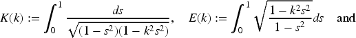
7.1. Complete Elliptic Integral

Let $k \in [0, 1)$ and $ν \in C$ . The complete elliptic integrals of the first, second and third kind are defined by

\begin{aligned} K (k) & := \int_{0}^{1} \frac{d s}{\sqrt{(1 - s^{2}) (1 - k^{2} s^{2})}}, E (k) := \int_{0}^{1} \sqrt{\frac{1 - k^{2} s^{2}}{1 - s^{2}}} d s and \end{aligned}

\begin{aligned} Π (ν, k) & := \int_{0}^{1} \frac{d s}{(1 + ν s^{2}) \sqrt{(1 - s^{2}) (1 - k^{2} s^{2})}}, \end{aligned}

(7.1)

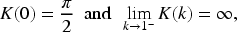
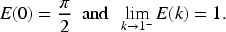
respectively. Then,

K (k)

is a monotone increasing function in

k

\begin{aligned} K (0) = \frac{π}{2} and lim_{k \to 1^{-}} K (k) = \infty, \end{aligned}

and

E (k)

is a monotone decreasing function in

k

\begin{aligned} E (0) = \frac{π}{2} and lim_{k \to 1^{-}} E (k) = 1. \end{aligned}

Lemma 7.1

Let $k \in (0, 1)$ . Then,

\begin{aligned} lim_{k \to 1^{-}} (K (k) - \log \frac{1}{\sqrt{1 - k^{2}}} - 2 \log 2) = 0. \end{aligned}

Therefore,

1 - k^{2} = 16 e^{- 2 K (k)} (1 + o (1))

k \to 1^{-}

See Byrd and Friedman (1971, Eq.112.01 in p.11) for Lemma 7.1.

7.2. Jacobi’s Elliptic Function

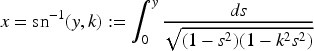
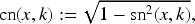
Let $k \in (0, 1)$ . Jacobi’s elliptic function $sn (x, k)$ is an odd, periodic and analytic function with the period $4 K (k)$ as a function for the real domain, and the inverse of $sn (x, k)$ is defined locally by

\begin{aligned} x = {sn}^{- 1} (y, k) := \int_{0}^{y} \frac{d s}{\sqrt{(1 - s^{2}) (1 - k^{2} s^{2})}} \end{aligned}

for

y \in [0, 1]

. The function

y = sn (x, k)

is a solution of

\begin{aligned} {\begin{cases} y^{″} + (1 + k^{2}) y - 2 k^{2} y^{3} = 0 & for x \in R, \\ y (0) = 0, y^{'} (0) = 1. \end{cases} \end{aligned}

The function

cn (x, k)

is an even and

4 K (k)

-periodic function defined locally by

\begin{aligned} cn (x, k) := \sqrt{1 - {sn}^{2} (x, k)}, \end{aligned}

for

x \in [0, K (k)]

. Then,

{sn}^{2} (x, k) + {cn}^{2} (x, k) = 1

. Moreover,

y (x) := cn (x, k)

is a solution of

\begin{aligned} {\begin{cases} y^{″} + (1 - 2 k^{2}) y + 2 k^{2} y^{3} = 0 & for x \in R, \\ y (0) = 1, y^{'} (0) = 0. \end{cases} \end{aligned}

The function

dn (ξ, k)

is an even and

2 K (k)

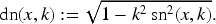
-periodic positive function defined by

\begin{aligned} dn (x, k) := \sqrt{1 - k^{2} {sn}^{2} (x, k)} . \end{aligned}

Then,

k^{2} {sn}^{2} (x, k) + {dn}^{2} (x, k) = 1

. Moreover,

y := dn (x, k)

is a solution of

\begin{aligned} {\begin{cases} y^{″} - (2 - k^{2}) y + 2 y^{3} = 0 & for x \in R, \\ y (0) = 1, y^{'} (0) = 0. \end{cases} \end{aligned}

Using the transformation $s = sn (x, k)$ in (7.1), we obtain the following expression of $Π (ν, k)$ :

\begin{aligned} Π (ν, k) = \int_{0}^{K (k)} \frac{d x}{1 + ν {sn}^{2} (x, k)}, \end{aligned}

where we used

\frac{d}{d x} sn x = cn x dn x

and

\sqrt{(1 - {sn}^{2} x) (1 - k^{2} {sn}^{2} x)} = cn x dn x

for

0 \leq x \leq K (k)

7.3. Weierstrass’s Elliptic Function

Let $k \in (0, 1)$ . In this paper we use Weierstrass’s elliptic function only of the following form:

\begin{aligned} ℘ (z; 2 ω_{1}, 2 ω_{3}) := \frac{1}{z^{2}} + \sum_{n^{2} + m^{2} \neq 0} {\frac{1}{(z - 2 m ω_{1} - 2 n ω_{3})^{2}} - \frac{1}{(2 m ω_{1} + 2 n ω_{3})^{2}}} \end{aligned}

for

z \in C

, where

\begin{aligned} ω_{1} := K (k) and ω_{3} := K (\sqrt{1 - k^{2}}) \sqrt{- 1} . \end{aligned}

The function

℘ (z)

has singularities at

z \in {2 m ω_{1} + 2 n ω_{3} \in C; (n, m) \in Z^{2}}

and it is a doubly periodic in the sense

\begin{aligned} ℘ (z + 2 ω_{1}) = ℘ (z) = ℘ (z + 2 ω_{3}) and ℘^{'} (z + 2 ω_{1}) = ℘^{'} (z) = ℘^{'} (z + 2 ω_{3}) \end{aligned}

Let

ω_{2} := - ω_{1} - ω_{3}

. We define

\begin{aligned} e_{1} := ℘ (ω_{1}), e_{2} := ℘ (ω_{2}) and e_{3} := ℘ (ω_{3}) . \end{aligned}

Then, it is known that

\begin{aligned} e_{1} = \frac{2 - k^{2}}{3} > 0, e_{2} = \frac{- 1 + 2 k^{2}}{3}, e_{3} = \frac{- 1 - k^{2}}{3} < 0, \end{aligned}

(7.2)

and hence

e_{3} < e_{2} < e_{1}

and

e_{1} + e_{2} + e_{3} = 0

. See Lawden (1989, Eq. (6.9.10) in p.163) for (7.2). Let

\begin{aligned} g_{2} := - 4 (e_{1} e_{2} + e_{2} e_{3} + e_{3} e_{1}) and g_{3} := 4 e_{1} e_{2} e_{3} . \end{aligned}

The following relation holds:

\begin{aligned} ℘^{'} {(z)}^{2} = 4 (℘ (z) - e_{1}) (℘ (z) - e_{2}) (℘ (z) - e_{3}) = 4 ℘ {(z)}^{3} - g_{2} ℘ (z) - g_{3} . \end{aligned}

These relations are used in the proof of Example 2.4. A reader can consult (Lawden, 1989, Chapter 6) for details of

℘ (z)

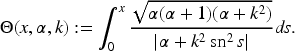
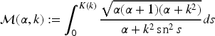
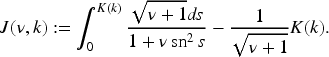
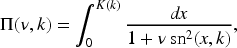
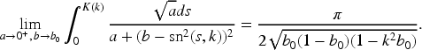
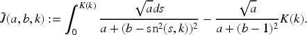
7.4. A Variant of the Complete Elliptic Integral of the Third Kind

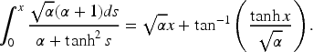
Let $k \in (0, 1)$ . We use the following variant of the complete elliptic integral of the third kind

\begin{aligned} M (α, k) := \int_{0}^{K (k)} \frac{\sqrt{α (α + 1) (α + k^{2})}}{α + k^{2} {sn}^{2} (s, k)} d s \end{aligned}

for

α \in (- 1, - k^{2}) \cup (0, \infty)

. Let

ν := k^{2} / α

. Then,

M

and

Π

have the following relation:

\begin{aligned} M (α, k) = sgn (ν) \sqrt{\frac{(ν + 1) (ν + k^{2})}{ν}} \int_{0}^{K (k)} \frac{d s}{1 + ν {sn}^{2} (s, k)} = sgn (ν) \sqrt{\frac{(ν + 1) (ν + k^{2})}{ν}} Π (ν, k) \end{aligned}

for

ν \in (- 1, - k^{2}) \cup (0, \infty)

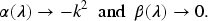
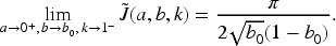
The function $M$ has the following limits at the end points of $(- 1, - k^{2}) \cup (0, \infty)$ .

Lemma 7.2

Let $k \in (0, 1)$ and $α \in (- 1, - k^{2}) \cup (0, \infty)$ . Then, the following hold:

(i) $lim_{α \to - 1} M (α, k) = 0$ .

(ii) $lim_{α \to - k^{2}} M (α, k) = - \frac{π}{2}$ .

(iii) $lim_{α \to 0} M (α, k) = \frac{π}{2}$ .

(iv) $lim_{α \to \infty} M (α, k) = \infty$ .

(i) and (iv) are trivial. Let $ν := k^{2} / α$ . (ii) follows from

\begin{aligned} lim_{ν \to - 1^{+}} \sqrt{1 + ν} Π (ν, k) = \frac{π}{2 \sqrt{1 - k^{2}}} . \end{aligned}

(7.3)

(iii) follows from

\begin{aligned} lim_{ν \to \infty} \sqrt{1 + ν} Π (ν, k) = \frac{π}{2} . \end{aligned}

(7.4)

See Wakasa and Yotsutani (2015, Lemma 7.4) for proofs of (7.3) and (7.4).

Lemma 7.3–7.6 are used to calculate the limit of eigenvalues. Those proofs can be found in Wakasa and Yotsutani (2015).

Lemma 7.3

Let

\begin{aligned} J (ν, k) := \int_{0}^{K (k)} \frac{\sqrt{ν + 1} d s}{1 + ν {sn}^{2} (s, k)} - \frac{K (k)}{\sqrt{ν + 1}} . \end{aligned}

(7.5)

Then,

\begin{aligned} lim_{ν \to \infty, k \to 1^{-}} J (ν, k) = \frac{π}{2} . \end{aligned}

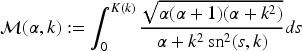
Lemma 7.4

Suppose that $α$ is a continuous function on $(0, 1)$ with $- 1 < α (k) < - k^{2}$ for $k \in (0, 1)$ . Assume that there exists $α^{*} \in [0, 1]$ such that

\begin{aligned} lim_{k \to 1^{-}} \frac{- α (k) - k^{2}}{1 - k^{2}} = α^{*} . \end{aligned}

Then,

\begin{aligned} lim_{k \to 1^{-}} M (α (k), k) = lim_{k \to 1^{-}} \int_{0}^{K (k)} \frac{\sqrt{α (k) (α (k) + 1) (α (k) + k^{2})}}{α (k) + k^{2} {sn}^{2} (s, k)} d s = - \frac{π}{2} + \tan^{- 1} \sqrt{\frac{α^{*}}{1 - α^{*}}} . \end{aligned}

Lemma 7.5

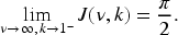
Suppose that $a > 0$ and $b, b_{0} \in (0, 1)$ . Then for each $k \in (0, 1)$ ,

\begin{aligned} lim_{a \to 0^{+}, b \to b_{0}} \int_{0}^{K (k)} \frac{\sqrt{a} d s}{a + (b - {sn}^{2} (s, k))^{2}} = \frac{π}{2 \sqrt{b_{0} (1 - b_{0}) (1 - k^{2} b_{0})}} . \end{aligned}

Lemma 7.6

Suppose that $a > 0$ , $b$ , $b_{0} \in (0, 1)$ and $k \in (0, 1)$ . Let

\begin{aligned} \tilde{J} (a, b, k) := \int_{0}^{K (k)} \frac{\sqrt{a} d s}{a + (b - {sn}^{2} (s, k))^{2}} - \frac{\sqrt{a}}{a + (b - 1)^{2}} K (k) . \end{aligned}

Then,

\begin{aligned} lim_{a \to 0^{+}, b \to b_{0}, k \to 1^{-}} \tilde{J} (a, b, k) = \frac{π}{2 \sqrt{b_{0}} (1 - b_{0})} . \end{aligned}

Footnotes

Acknowledgments

YM was supported by JSPS KAKENHI Grant Number 24K00530. KT was supported by JSPS KAKENHI Grant Number 22K03368. TW was supported by JSPS KAKENHI Grant Number 24K06814.

ORCID iDs

Yasuhito Miyamoto

Kouichi Takemura

Tohru Wakasa

Funding

The authors received no financial support for the research, authorship and/or publication of this article.

Declaration of Conflicting Interests

The authors declared no potential conflicts of interest with respect to the research, authorship, and/or publication of this article.

Data Availability

Data sharing is not applicable to this article as no new data were created or analyzed in this study.

References

Aizawa

Miyamoto

Wakasa

(2023). Asymptotic formulas of the eigenvalues for the linearization of a one-dimensional sinh-poisson equation. Journal of Elliptic and Parabolic Equations, 9, 1043–1070.

Arscott

(1964). Periodic differential equations: An introduction to mathieu, lamé, and allied functions. International series of monographs in pure and applied mathematics (vol. 66). The Macmillan Company x+284 pp.

Byrd

Friedman

(1971). Handbook of elliptic integrals for engineers and scientists, Die grundlehren Der Mathematischen Wissenschaften (2nd ed., Vol. 67). Springer-Verlag.

Carr

Pego

(1989). Metastable patterns in solutions of

u_{t} = ϵ^{2} u_{x x} - f (u)

. Communications on Pure and Applied Mathematics, 42, 523–576.

de Groen

Karadzhov

(2002). Metastability in the shadow system for Gierer–Meinhardt’s equations. Electronic Journal of Differential Equations, 2002, 22.

Eckmann

Rougemont

(1998). Coarsening by ginzburg-landau dynamics. Communications in Mathematical Physics, 199, 441–470.

Funakubo

Otsuki

Toyoda

(1990). Sphalerons of

O (3)

nonlinear sigma model on a circle. Progress of Theoretical Physics, 83, 118–133.

Iron

Ward

(2000). A metastable spike solution for a nonlocal reaction-diffusion model. SIAM Journal on Applied Mathematics, 60, 778–802.

Lawden

(1989). Elliptic functions and applications. Applied mathematical sciences (Vol. 80). Springer-Verlag. xiv+334 pp. ISBN: 0-387-96965-9.

10.

Liang

Müller-Kirsten

Tchrakian

(1992). Solitons, bounces and sphalerons on a circle. Physics Letters B, 282, 105–110.

11.

Magnus

Winkler

(1966). Hill’s Equation, Interscience Tracts in Pure and Applied Mathematics, No. 20. Interscience Publishers John Wiley & Sons. viii+127 pp.

12.

Manton

Samols

(1988). Sphalerons on a circle. Physics Letters B, 207, 179–184.

13.

Miyamoto

Takemura

Wakasa

(2023). Asymptotic formulas of the eigenvalues for the linearization of the scalar field equation. Proceedings of the Royal Society of Edinburgh Section A: Mathematics, 155, 307–344.

14.

Miyamoto

Wakasa

(2019). Exact eigenvalues and eigenfunctions for a one-dimensional Gel’fand problem. Journal of Mathematical Physics, 60, 021506.

15.

Smondyrev

Vansant

Peeters

Devreese

(1995). Nonlinear Schrödinger equation on a circle. Physical Review B, 52, 231–237.

16.

Takemura

(2003). The Heun equation and the Calogero–Moser–Sutherland system. I. The bethe ansatz method. Communications in Mathematical Physics, 235, 467–494.

17.

Takemura

(2004). The Heun equation and the Calogero–Moser–Sutherland system. III. The finite gap property and the monodromy. Journal of Nonlinear Mathematical Physics, 11, 21–46.

18.

Takemura

(2005). The Heun equation and the Calogero–Moser–Sutherland system. IV. The Hermite–Krichever ansatz. Communications in Mathematical Physics, 258, 367–403.

19.

Takemura

(2006). On eigenvalues of Lamé operator. Sūrikaisekikenkyūsho Kōkyūroku, 1480, 104–116.

20.

Takemura

(2007). Towards finite-gap integration of the inozemtsev model. Symmetry, Integrability and Geometry: Methods and Applications, 3, 038.

21.

Wakasa

(2006). Exact eigenvalues and eigenfunctions associated with linearization for Chafee–Infante problem. Funkcialaj Ekvacioj, 49, 321–336.

22.

Wakasa

Yotsutani

(2008). Representation formulas for some 1-dimensional linearized eigenvalue problems. Communications on Pure and Applied Mathematics, 7, 745–763.

23.

Wakasa

Yotsutani

(2015). Limiting classification on linearized eigenvalue problems for 1-dimensional Allen–Cahn equation I-asymptotic formulas of eigenvalues. Journal of Differential Equations, 258, 3960–4006.

24.

Whittaker

Watson

(1927). A course of modern analysis. An introduction to the general theory of infinite processes and of analytic functions; With an account of the principal transcendental functions. Reprint of the fourth edition, Cambridge mathematical library. Cambridge University Press.