Asymptotic Expansions for the Transmission Eigenvalues of Periodic Scatterers of Bounded Support

Abstract

We consider the transmission eigenvalues for a bounded scatterer with a periodically varying index of refraction, and derive the first-order corrections to the limiting transmission eigenvalues. We assume the scatterer contrast to be of one sign, in which case the transmission eigenvalue problem can be written in terms of operators corresponding to a fourth-order partial differential equation with periodic coefficients. We perform two scale asymptotics for this biharmonic-type homogenization problem and show convergence estimates, which require a boundary corrector function, and this boundary corrector function appears in the formula for the transmission eigenvalues correction.

Keywords

homogenization transmission eigenvalues fourth-order elliptic scattering theory boundary correctors

1. Introduction

The transmission eigenvalue problem plays a fundamental role in scattering theory for inhomogeneous media. Transmission eigenvalues correspond to interrogating frequencies at which there exists an incident field that does not scatter by the medium. Despite its deceptively simple formulation—two elliptic partial differential equations (PDEs) in a bounded domain (one governing wave propagation in the scattering medium and the other in the background that occupies the support of the medium) that share the same Cauchy data on the boundary—the problem presents a remarkably intricate mathematical structure. In particular, it is a non-self-adjoint eigenvalue problem for a non-strongly elliptic operator, making the investigation of its spectral properties highly challenging. We refer the reader to Cakoni et al. (2023) for the significance of this problem in scattering phenomena and inverse scattering theory.

More precisely, let $n (x)$ denote the refractive index of an inhomogeneous medium of bounded support, which is a perturbation of the homogeneous background medium with refractive index scaled to one. Define $\bar{D} := supp (n - 1)$ . The transmission eigenvalue problem is then formulated as finding $v \neq 0$ and $w \neq 0$ satisfying

\begin{aligned} {\begin{aligned} Δ w + k^{2} n (x) w & = 0 in D, \\ Δ v + k^{2} v & = 0 in D, \\ w - v & = 0 on \partial D, \\ \frac{\partial w}{\partial ν} - \frac{\partial v}{\partial ν} & = 0 on \partial D, \end{aligned} \end{aligned}

(1)

where

k > 0

is the wave number, proportional to the interrogating frequency

ω

. In this formulation,

u := w - v

corresponds to the scattered field, which by virtue of the boundary conditions (provided

\partial D

has some regularity), can be extended by zero into the exterior of

D

, whereas

v

is the restriction to

D

of the incoming incident wave. This formulation shows that a necessary condition for an incident wave to remain unscattered by the inhomogeneity

(D, n)

is the existence of a nontrivial solution to (1). The transmission eigenvalue problem is known to be non-self-adjoint (Cakoni et al., 2023), and complex transmission eigenvalues may occur, although only the real ones are physically relevant to nonscattering. Values of

k \in C

for which (1) admits nontrivial solutions

(w, v)

are called transmission eigenvalues. Note that it can be shown that real transmission eigenvalues can be determined from measured scattering data (Cakoni, Colton, et al., 2010, 2023; Kirsch & Lechleiter, 2013), hence they can be used to determine information about refractive index

n

when solving the inverse scattering problem. There is a vast literature on the spectral analysis of the transmission eigenvalue problem. The discreteness of the spectrum, completeness of eigenfunctions, and Weyl’s asymptotics have been established under various assumptions on

n - 1

in Fornerod and Nguyen (2023), Kirsch (2016), Robbiano (2013), and Vodev (2018, 2025). In particular, if

n - 1

has a fixed sign uniformly in

D

, then there exists an infinite sequence of real transmission eigenvalues accumulating only at

+ \infty

Figure 1.

Inhomogeneity $D$ of bounded support with periodic refractive index $n (x / ϵ)$ with period cell of size $ϵ$ .

In this work, we deal with the perturbation analysis of transmission eigenvalues when the inhomogeneous medium $(D, n)$ , with $D \subset R^{d}$ for $d = 2, 3$ bounded, is periodic and highly oscillating. More precisely, let $ϵ > 0$ denote the characteristic size of the periodic unit cell, which is assumed to be small relative to the size of $D$ , and let $Y = [0, 1]^{d}$ be the rescaled unit cell. We assume that the refractive index is given by

\begin{aligned} n_{ϵ} (x) := n (x / ϵ) \in L^{\infty} (D), \end{aligned}

with

n

periodic in

y = x / ϵ

with period

Y

. That is, inside

D

n_{ϵ}

is the restriction of a periodic function with cell size

ϵ

to the bounded domain

D

, while outside of

D

n_{ϵ} \equiv 1

. We note that the domain

D

does not itself depend on

ϵ

. See Figure 1 for a sketch of the geometry. Our concern is how the real transmission eigenvalues perturb as

ϵ \to 0

. The homogenization theory for the corresponding direct scattering problem has been developed in Cakoni et al. (2019, 2020), while the convergence of the real transmission eigenvalues to those of the homogenized medium was proven in Cakoni, Haddar, et al. (2015). The main goal of this paper is to provide an explicit first-order correction term in the asymptotic expansion of the real transmission eigenvalue. Since the correction to the homogenized transmission eigenvalue can be determined, the hope is that this correction term captures microstructural information of the periodic medium. Such asymptotic analyses have been carried out for transmission eigenvalue problems in media containing small-size perturbations as the perturbation size tends to zero in Cakoni, Moskow, et al. (2015) and Cakoni et al. (2017). Our perturbation analysis is based on the work of Osborn (1975), extended to nonlinear eigenvalue problems in Moskow (2015) and Furia and Moskow (2025). In particular, our approach makes use of the expression given in Furia and Moskow (2025).

In this paper, we formulate the transmission eigenvalue problem as a nonlinear eigenvalue problem for a fourth-order partial differential operator given by (10). Using two scale asymptotics for the resolvent of the bi-Laplacian-type operator, we establish higher-order convergence estimates as $ϵ \to 0$ . While homogenization for periodic higher-order PDEs is known (Francfort, 1992; Niu et al., 2018; Niu & Xu, 2019; Pastukhova, 2017), these higher-order estimates, including boundary corrector functions, appear to be new. We show first that the homogenized problem reduces to the eigenvalue problem with cell-averaged refractive index $\bar{n}$ , recovering (Cakoni, Haddar, et al., 2015). We then construct higher-order correctors: the first-order expansion includes only a boundary correction (consistent with the homogenization of direct scattering problems Cakoni et al., 2019, 2020), while higher orders involve both bulk and boundary terms. The resolvent estimates yield asymptotics for simple real transmission eigenvalues, based on the formula in Furia and Moskow (2025, Theorem 3.2). The leading correction involves the boundary corrector integrated against the scaled eigenfunction. The boundary corrector satisfies a fourth-order boundary value problem with oscillatory coefficients, and it is highly desirable to understand the limiting behavior of the boundary corrector as $ϵ \to 0$ . This is a delicate issue in the theory of homogenization, and for the state-of-the-art of this question for second-order PDEs is discussed in Gérard-Varet and Masmoudi (2011, 2012), Moskow and Vogelius (1997a), and Santosa and Vogelius (1993). Here, although we can prove that the boundary corrector is $L^{2}$ -bounded with respect to $ϵ$ , and thus admits weak subsequential limit(s), we characterize its (nonzero) limit only in one dimension. We find that the first-order corrections are not unique and depend on the interaction of the boundary of the scatterer with the microstructure. The two- and three-dimensional cases, which are technically more involved, will be addressed in a subsequent paper.

2. Description of Problem

We assume that the bounded domain $D \subset R^{d}$ has $C^{2}$ boundary, and as stated in the introduction, we assume that $n (y)$ is a bounded periodic function of $y$ in the cell $Y = [0, 1]^{d}$ . Let $H_{0}^{2} (D)$ denote the Sobolev space given by

\begin{aligned} H_{0}^{2} (D) := {u \in H^{2} (D) : u = \frac{\partial u}{\partial ν} = 0 on \partial D}, \end{aligned}

or, equivalently, the

H^{2}

closure of

C_{0}^{\infty} (D)

functions, equipped with the inner product

\begin{aligned} (u, v)_{H_{0}^{2} (D)} = (Δ u, Δ v)_{L^{2} (D)} . \end{aligned}

Consider now the interior transmission eigenvalue problem (1) formulated above, which has a periodic coefficient with period

ϵ > 0

, small compared to its support

D

. Letting

τ := k^{2}

, we wish to find nontrivial

w, v \in L^{2} (D)

with

w - v \in H_{0}^{2} (D)

satisfying

\begin{aligned} Δ w + τ n (x / ϵ) w & = 0 in D, \end{aligned}

(2)

\begin{aligned} Δ v + τ v & = 0 in D, \end{aligned}

(3)

\begin{aligned} w & = v on \partial D, \end{aligned}

(4)

\begin{aligned} \frac{\partial w}{\partial ν} & = \frac{\partial v}{\partial ν} on \partial D . \end{aligned}

(5)

Note that the boundary conditions are equivalent to saying that

w - v \in H_{0}^{2} (D)

. Here the eigenvalue parameter is

τ := k^{2}

. As already mentioned, the transmission eigenvalue problem is not self-adjoint, and in the spherical symmetric case it is known to have complex eigenvalues (Cakoni et al., 2023, Chapter 6). Here, we are concerned only with the real transmission eigenvalue, since they are the ones which can be measured from scattering data. More precisely, here transmission eigenvalues refer to values of

τ \in R_{+}

for which the problems (2)–(5) have a nontrivial solution. In this work, we limit ourselves to the case when

n (x / ϵ) - 1

is of one sign, and for the calculations, we assume that

n (x / ϵ) - 1 \geq c > 0

, with

c

independent of

ϵ

. In this case, an infinite number of real transmission eigenvalues are known to exist (Cakoni, Gintides, et al., 2010). We are interested in the behavior of these transmission eigenvalues as the period size

ϵ

approaches zero. It is known from the work (Cakoni, Haddar, et al., 2015) that the real transmission eigenvalues

{λ_{ϵ}}

(omitting indexing) converge to those corresponding to

{λ_{0}}

for the “homogenized” transmission eigenvalue problem, that is, those corresponding to

\begin{aligned} Δ w + τ \bar{n} w & = 0 in D, \end{aligned}

(6)

\begin{aligned} Δ v + τ v & = 0 in D \end{aligned}

(7)

\begin{aligned} w & = v on \partial D, \end{aligned}

(8)

\begin{aligned} \frac{\partial w}{\partial ν} & = \frac{\partial v}{\partial ν} on \partial D, \end{aligned}

(9)

where

\bar{n}

denotes the period cell average

\begin{aligned} \bar{n} = \frac{1}{| Y |} \int_{Y} n (y) d y . \end{aligned}

Our motivation here is to find the next order term, that is, the corrections

τ^{(1)}

, where each

\begin{aligned} τ_{ϵ} = τ_{0} + ϵ τ^{(1)} + o (ϵ) . \end{aligned}

From the work (Cakoni, Gintides, et al., 2010), for this setup, we have that the transmission eigenvalue problem (2) is equivalent to the fourth-order nonlinear eigenvalue problem: Find $τ$ such that there exist nontrivial $u = w - v \in H_{0}^{2} (D)$ , such that

\begin{aligned} (Δ + τ n_{ϵ}) \frac{1}{n_{ϵ} - 1} (Δ + τ) u = 0, \end{aligned}

(10)

where we use

n_{ϵ}

to denote the periodic

\begin{aligned} n_{ϵ} = n (x / ϵ) . \end{aligned}

We can state this in variational form as follows: Find

u \in H_{0}^{2} (D)

such that

\begin{aligned} \int_{D} \frac{1}{n_{ϵ} - 1} (Δ u + τ u) (Δ ϕ + τ n_{ϵ} ϕ) d x = 0 for all ϕ \in H_{0}^{2} (D) . \end{aligned}

(11)

Following Cakoni, Gintides, et al. (2010), we rewrite this in terms of variationally defined operators. Let us define the bounded bilinear forms on

H_{0}^{2} (D) \times H_{0}^{2} (D)

\begin{aligned} A_{τ, ϵ} (u, ϕ) = {(\frac{1}{n_{ϵ} - 1} (Δ u + τ u), (Δ ϕ + τ ϕ))}_{L^{2} (D)} + τ^{2} (u, ϕ)_{L^{2} (D)} \end{aligned}

(12)

and

\begin{aligned} B (u, ϕ) = (\nabla u, \nabla ϕ)_{L^{2} (D)} . \end{aligned}

(13)

By the Riesz representation theorem, these bilinear forms define bounded operators

A_{τ, ϵ} : H_{0}^{2} (D) \to H_{0}^{2} (D)

and

B : H_{0}^{2} (D) \to H_{0}^{2} (D),

which are such that

\begin{aligned} A_{τ, ϵ} (u, ϕ) = (A_{τ, ϵ} u, ϕ)_{H_{0}^{2} (D)} and B (u, ϕ) = (B u, ϕ)_{H_{0}^{2} (D)}, \end{aligned}

(14)

for all

u, ϕ \in H_{0}^{2} (D)

. We may also find it convenient to write these variationally defined operators using PDE notation. For given

f \in H^{2} (D)

, we have that

\begin{aligned} A_{τ, ϵ}^{- 1} f = {((Δ + τ) \frac{1}{n_{ϵ} - 1} (Δ + τ) + τ^{2})}^{- 1} Δ Δ f \end{aligned}

and

\begin{aligned} B f = (Δ Δ)^{- 1} Δ f, \end{aligned}

where the inverses of the fourth-order operators have range in

H_{0}^{2} (D)

, where solutions are unique. We also note that the operator

B : H^{2} (D) \to H_{0}^{2} (D)

has a bounded extension on

L^{2} (D)

; for any

f \in L^{2} (D)

Δ f

is understood in the sense of

H^{- 2} (D)

, the dual of

H_{0}^{2} (D)

. We continue to use

B

to denote this operator

B : L^{2} (D) \to H_{0}^{2} (D)

, so that

B

is clearly compact from

L^{2} (D)

to itself. Furthermore,

A_{τ, ϵ}

is invertible on

H_{0}^{2} (D)

for positive real

τ

, and the coercivity constant is independent of

τ

(Cakoni & Haddar, 2009). The variational form (11) of the transmission eigenvalue problem is equivalent to finding

u \in L^{2} (D)

such that

\begin{aligned} (I - τ A_{τ, ϵ}^{- 1} B) u = 0. \end{aligned}

(15)

Define the linear operator

T_{ϵ} (τ) : L^{2} (D) \to L^{2} (D)

for

ϵ \geq 0

and

τ \in C

such that

\begin{aligned} T_{ϵ} (τ) & := A_{τ, ϵ}^{- 1} B \\ = {((Δ + τ) \frac{1}{n_{ϵ} - 1} (Δ + τ) + τ^{2})}^{- 1} Δ, \end{aligned}

(16)

so we can write (15) as

\begin{aligned} τ T_{ϵ} (τ) u = u, \end{aligned}

(17)

and its limiting problem

\begin{aligned} τ T_{0} (τ) u = u . \end{aligned}

(18)

Here

T_{0}

is defined as

\begin{aligned} T_{0} (τ) & := A_{τ, 0}^{- 1} B \\ = {((Δ + τ) \frac{1}{\bar{n} - 1} (Δ + τ) + τ^{2})}^{- 1} Δ, \end{aligned}

(19)

where

A_{τ, 0}

is defined as in (14), but with

n_{ϵ}

replaced with its limiting value

n_{0} = \bar{n}

We have now rephrased the problem as a nonlinear eigenvalue perturbation problem. That is, a transmission eigenvalue $τ_{ϵ}$ is a value for $τ$ such that there exists a nontrivial $u \in L^{2} (D)$ satisfying

\begin{aligned} τ_{ϵ} T_{ϵ} (τ_{ϵ}) u = u \end{aligned}

for

ϵ > 0

. A limiting transmission eigenvalue is a value

τ_{0}

such that there exists nontrivial

u \in L^{2} (D)

, such that

\begin{aligned} τ_{0} T_{0} (τ_{0}) u = u . \end{aligned}

In order to find a correction formula for the transmission eigenvalues of the perturbed problem in terms of the eigenvalues and eigenvectors of the background problem, we will apply a result in Moskow (2015), an application of Osborn’s theorem for approximating the eigenvalues of compact operators (Osborn, 1975). Let

τ_{ϵ}

be the eigenvalue associated with the nonlinear eigenvalue problem (17) and let

τ_{0}

be the eigenvalue corresponding to the limiting eigenvalue problem (18). In this paper, we will derive an expression for the next order correction term

τ^{(1)}

in the asymptotic expansion

\begin{aligned} τ_{ϵ} = τ_{0} + ϵ τ^{(1)} + o (ϵ) . \end{aligned}

Remark 1

For the sake of presentation, we present the calculations for the case when $n_{ϵ} > 1$ uniformly in $D$ . A similar analysis can be done in the case $0 < n_{ϵ} < 1$ uniformly in $D$ . In this case, the definition of the coercive part (12) is replaced (see Cakoni et al., 2023, Section 4.2)

\begin{aligned} {\tilde{A}}_{τ, ϵ} (u, ϕ) = {(\frac{1}{1 - n_{ϵ}} (Δ u + τ n_{ϵ} u), (Δ ϕ + τ n_{ϵ} ϕ))}_{L^{2} (D)} + τ^{2} (n_{ϵ} u, ϕ)_{L^{2} (D)}, \end{aligned}

with the corresponding operators defined accordingly.

3. Operator Convergence: A Fourth-Order Homogenization Problem

In order to apply the eigenvalue correction theorem, we will need to explore the convergence of $T_{ϵ} (τ)$ to $T_{0} (τ)$ , or more precisely, we will need an asymptotic expansion with respect to $ϵ$ for $T_{ϵ} (τ)$ and corresponding norm estimates. We need to focus on $A_{τ, ϵ}^{- 1}$ , since all of the $ϵ$ dependence is in this operator. Note that if

\begin{aligned} u_{ϵ} = A_{τ, ϵ}^{- 1} f, \end{aligned}

then

u_{ϵ} \in H_{0}^{2} (D)

is the variational solution to

\begin{aligned} (Δ + τ) \frac{1}{n (x / ϵ) - 1} (Δ + τ) u_{ϵ} + τ^{2} u_{ϵ} = Δ Δ f in D, \end{aligned}

(20)

where

n (y)

is periodic on the period cell

Y

. For simplicity of exposition, we let

\begin{aligned} a (x / ϵ) = \frac{1}{n (x / ϵ) - 1} \end{aligned}

(21)

and

\begin{aligned} h = Δ Δ f, \end{aligned}

so that

u_{ϵ} \in H_{0}^{2} (D)

solves

\begin{aligned} (Δ + τ) a (x / ϵ) (Δ + τ) u_{ϵ} + τ^{2} u_{ϵ} = h in D; \end{aligned}

(22)

the periodic homogenization problem, which is the subject of this section. We note that such fourth-order periodic problems have been studied in the past, see, for example, Pastukhova (2017) and Francfort (1992), and so the expansion of the main part of the operator is not new. Here, we focus on obtaining high enough order

L^{2}

norm estimates, which we will need to apply the eigenvalue perturbation theorem. These estimates require the introduction and analysis of a fourth-order boundary corrector function.

3.1. Formal Asymptotics

We proceed by assuming that $a (y) \geq a_{0} > 0$ is positive, bounded in $L^{\infty}$ , and periodic, and we do standard two scale asymptotic expansions. Let $y = x / ϵ$ so that from the chain rule

\begin{aligned} \nabla = \nabla_{x} + \frac{1}{ϵ} \nabla_{y}, \end{aligned}

and assume the ansatz for the solution

u_{ϵ}

of (22)

\begin{aligned} u_{ϵ} \approx u_{0} (x, y) + ϵ u^{(1)} (x, y) + ϵ^{2} u^{(2)} (x, y) + \dots, \end{aligned}

(23)

where each

u^{(i)} (x, y)

is periodic in the fast variable

y

in the sense of

H_{♯}^{2} (Y)

, where

H_{♯}^{2} (Y)

is defined to be

H^{2}

functions on the torus, defined in terms of the decay of the Fourier coefficients. Equivalently, this is all

H^{2} (Y)

functions, which are also in

H^{2}

across the matching boundaries (the closure of smooth functions on the torus in the

H^{2}

norm). We note that

\begin{aligned} Δ = Δ_{x} + \frac{2}{ϵ} \nabla_{y} \cdot \nabla_{x} + \frac{1}{ϵ^{2}} Δ_{y} . \end{aligned}

We could proceed by plugging the ansatz (23) into (22); however, we will instead rewrite (22) as a second-order system. The use of a lower-order system both simplifies the derivation of the terms in the ansatz and potentially allows for lower regularity assumptions. To this end, we let

v_{ϵ} = a (x / ϵ) (Δ + τ) u_{ϵ}

so that the pair

(u_{ϵ}, v_{ϵ})

solves

\begin{aligned} a (x / ϵ) (Δ + τ) u_{ϵ} & = v_{ϵ}, \end{aligned}

(24)

\begin{aligned} (Δ + τ) v_{ϵ} + τ^{2} u_{ϵ} & = h, \end{aligned}

and so we also expand

\begin{aligned} v_{ϵ} \approx v_{0} (x, y) + ϵ v^{(1)} (x, y) + ϵ^{2} v^{(2)} (x, y) + \dots . \end{aligned}

(25)

We plug the ansatz into the system,

\begin{aligned} a (y) (Δ_{x} + \frac{2}{ϵ} \nabla_{y} \cdot \nabla_{x} + \frac{1}{ϵ^{2}} Δ_{y} + τ) (u_{0} + ϵ u^{(1)} + ϵ^{2} u^{(2)} + \dots) \\ = v_{0} + ϵ v^{(1)} + ϵ^{2} v^{(2)} + \dots (Δ_{x} + \frac{2}{ϵ} \nabla_{y} \cdot \nabla_{x} + \frac{1}{ϵ^{2}} Δ_{y} + τ) \\ \times (v_{0} + ϵ v^{(1)} + ϵ^{2} v^{(2)} + \dots) + τ^{2} (u_{0} + ϵ u^{(1)} + ϵ^{2} u^{(2)} + \dots) = h, \end{aligned}

(26)

and set equal the coefficients of like powers of epsilon to obtain the equations

\begin{matrix} \begin{aligned} \frac{1}{ϵ^{2}} : a Δ_{y} u_{0} & = 0, \\ Δ_{y} v_{0} & = 0, \end{aligned} \end{matrix}

(27)

\begin{matrix} \begin{aligned} \frac{1}{ϵ} : 2 a \nabla_{x} \nabla_{y} u_{0} + a Δ_{y} u^{(1)} & = 0, \\ 2 \nabla_{x} \nabla_{y} v_{0} + Δ_{y} v^{(1)} & = 0, \end{aligned} \end{matrix}

(28)

\begin{matrix} \begin{aligned} ϵ^{0} : a (Δ_{x} + τ) u_{0} + 2 a \nabla_{x} \cdot \nabla_{y} u^{(1)} + a Δ_{y} u^{(2)} & = v_{0}, \\ (Δ_{x} + τ) v_{0} + 2 \nabla_{x} \cdot \nabla_{y} v^{(1)} + Δ_{y} v^{(2)} + τ^{2} u_{0} & = h, \end{aligned} \end{matrix}

(29)

\begin{matrix} \begin{aligned} ϵ : a (Δ_{x} + τ) u^{(1)} + 2 a \nabla_{x} \cdot \nabla_{y} u^{(2)} + a Δ_{y} u^{(3)} & = v^{(1)}, \\ (Δ_{x} + τ) v^{(1)} + 2 \nabla_{x} \cdot \nabla_{y} v^{(2)} + Δ_{y} v^{(3)} + τ^{2} u^{(1)} & = 0, \end{aligned} \end{matrix}

(30)

\begin{matrix} \begin{aligned} ϵ^{2} : a (Δ_{x} + τ) u^{(2)} + 2 a \nabla_{x} \cdot \nabla_{y} u^{(3)} + a Δ_{y} u^{(4)} & = v^{(2)}, \\ (Δ_{x} + τ) v^{(2)} + 2 \nabla_{x} \cdot \nabla_{y} v^{(3)} + Δ_{y} v^{(4)} + τ^{2} u^{(2)} & = 0, \end{aligned} \end{matrix}

(31)

and, in general, for

n \geq 1

, the equation corresponding to

ϵ^{n}

\begin{aligned} ϵ^{n} : a (Δ_{x} + τ) u^{(n)} + 2 a \nabla_{x} \cdot \nabla_{y} u^{(n + 1)} + a Δ_{y} u^{(n + 2)} & = v^{(n)}, \end{aligned}

(32)

\begin{aligned} (Δ_{x} + τ) v^{(n)} + 2 \nabla_{x} \cdot \nabla_{y} v^{(n + 1)} + Δ_{y} v^{(n + 2)} + τ^{2} u^{(n)} & = 0. \end{aligned}

First, we observe that the first two sets of equations (27) and (28) imply that the first terms do not depend on

y

, that is,

u_{0} = u_{0} (x)

v_{0} = v_{0} (x)

u^{(1)} = u^{(1)} (x)

, and

v^{(1)} (x) = v_{0} (x)

. Since

v_{0} (x)

does not depend on

y

, the first equation in (29) suggests that we should take

\begin{aligned} u^{(2)} (x, y) = χ (y) (Δ_{x} + τ) u_{0} (x), \end{aligned}

(33)

where

\begin{aligned} a + a Δ_{y} χ = c, \end{aligned}

for some constant

c

. Periodicity implies that we must have

c = {\bar{a^{- 1}}}^{- 1}

, leading to

\begin{aligned} Δ_{y} χ (y) = {\bar{a^{- 1}}}^{- 1} / a - 1. \end{aligned}

(34)

We note that a priori

u^{(2)}

could still have an additive function of

x

. Taking the

Y

cell average of (29) and using the formula for

χ

, we find the homogenized problem

\begin{aligned} (Δ_{x} + τ) {\bar{a^{- 1}}}^{- 1} (Δ_{x} + τ) u_{0} + τ^{2} u_{0} = h, \end{aligned}

(35)

accompanied by

\begin{aligned} v_{0} = {\bar{a^{- 1}}}^{- 1} (Δ_{x} + τ) u_{0} . \end{aligned}

(36)

Now, if we take

\begin{aligned} u^{(3)} = \vec{γ} (y) \cdot \nabla_{x} (Δ_{x} + τ) u_{0}, \end{aligned}

(37)

where the vector

\vec{γ}

has cell average zero and solves

\begin{aligned} - Δ_{y} \vec{γ} = 2 \nabla_{y} χ (y), \end{aligned}

(38)

we see that the first equation of (30) is satisfied with

\begin{aligned} u^{(1)} = v^{(1)} = 0. \end{aligned}

The second equation of (30) is also satisfied if we take

\begin{aligned} v^{(2)} = v^{(3)} = 0. \end{aligned}

If we do this, to satisfy the first equation of (31), we can take

\begin{aligned} u^{(4)} = α (y) (Δ_{x} + τ) (Δ_{x} + τ) u_{0} + B_{i j} (y) (D_{x}^{2})_{i j} (Δ_{x} + τ) u_{0}, \end{aligned}

(39)

where the

α (y)

has cell average zero and solves

\begin{aligned} - Δ_{y} α = χ, \end{aligned}

(40)

and matrix

B (y)

has components with cell average zero satisfying

\begin{aligned} - Δ_{y} B_{i j} = 2 \frac{\partial γ_{i}}{\partial y_{j}} . \end{aligned}

(41)

In (39), Einstein summation notation is employed, with

D^{2}

denoting the Hessian. We find then to satisfy the second equation in (31), we need a nonzero

v^{(4)}

, and taking

\begin{aligned} v^{(4)} = τ^{2} α (y) (Δ_{x} + τ) u_{0} \end{aligned}

(42)

will work. To summarize, we have thus far derived

\begin{aligned} u_{ϵ} & \approx u_{0} + ϵ^{2} u^{(2)} + ϵ^{3} u^{(3)} + ϵ^{4} u^{(4)} \dots, \end{aligned}

\begin{aligned} v_{ϵ} & \approx v_{0} + ϵ^{4} v^{(4)} + \dots, \end{aligned}

with

u^{(2)}

u^{(3)}

u^{(4)}

v_{0}

, and

v^{(4)}

given by (33), (37), (39), (36), and (42), respectively. We need to emphasize, however, that beyond second order these choices are not necessarily optimal; there may be other third- and fourth-order terms necessary if one wanted estimates of higher order.

Our solutions $u_{ϵ}$ and $u_{0}$ are in $H_{0}^{2} (D)$ , but due to the corrections, our approximation to $u_{ϵ}$ is no longer in $H_{0}^{2} (D)$ . Hence, in order to obtain high enough order convergence estimates, will need the boundary corrector functions at each order. Let $θ_{ϵ}^{(n)}$ denote the unique $H^{2} (D)$ solution to

\begin{aligned} (Δ_{x} + τ) a (x / ϵ) (Δ + τ) θ_{ϵ}^{(n)} + τ^{2} θ_{ϵ}^{(n)} & = 0 in D, \end{aligned}

(43)

\begin{aligned} θ_{ϵ}^{(n)} & = - ϵ u^{(n)} on \partial D, \\ \frac{\partial θ_{ϵ}^{(n)}}{\partial ν} & = - ϵ \frac{\partial u^{(n)}}{\partial ν} on \partial D, \end{aligned}

and define its second-order system counterpart

\begin{aligned} ψ_{ϵ}^{(n)} = a (x / ϵ) (Δ + τ) θ_{ϵ}^{(n)} . \end{aligned}

(44)

Then, the pair

(θ_{ϵ}^{(n)}, ψ_{ϵ}^{(n)})

solves

\begin{aligned} a (x / ϵ) (Δ + τ) θ_{ϵ}^{(n)} & = ψ_{ϵ}^{(n)}, \end{aligned}

(45)

\begin{aligned} (Δ + τ) ψ_{ϵ}^{(n)} + τ^{2} θ_{ϵ}^{(n)} & = 0. \end{aligned}

Remark 2

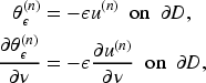
Since for our transmission eigenvalue problem $a = 1 / (n - 1)$ , we have that

\begin{aligned} Δ_{y} χ (y) = \frac{n (y) - \bar{n}}{\bar{n} - 1}, \end{aligned}

(46)

which means that

\begin{aligned} χ = \frac{β}{\bar{n} - 1}, \end{aligned}

where

β

is the first-order cell function from the homogenization of the standard transmission problem corresponding to

n

; which is

Y

-periodic, has cell average zero, and solves

\begin{aligned} Δ_{y} β (y) = n (y) - \bar{n}, \end{aligned}

(47)

see, for example, Cakoni et al. (2019, 2020).

3.2. Norm Estimates

We note that for all of the two scale functions, including the boundary data for $θ_{ϵ}^{(n)} (x)$ , we set $y = x / ϵ$ , and subsequently all resulting approximations and errors are considered as functions of the single variable $x \in D$ . The following lemma will be useful for showing convergence estimates.

Lemma 1
Assume that $z_{ϵ}, η_{ϵ}$ are in $H_{0}^{2} (D)$ and $L^{2} (D)$ , respectively, and that they satisfy the second-order system
$\begin{aligned} a (x / ϵ) (Δ + τ) z_{ϵ} - η_{ϵ} & = e, \end{aligned}$
(48)

$\begin{aligned} (Δ + τ) η_{ϵ} + τ^{2} z_{ϵ} & = f . \end{aligned}$
Then, there exists $C$ independent of $ϵ$ such that
$\begin{aligned} ‖ z_{ϵ} ‖_{H_{0}^{2} (D)} \leq C (‖ e ‖_{L^{2} (D)} + ‖ f ‖_{H^{- 2} (D)}) . \end{aligned}$
(49)
Proof.
Consider
$\begin{aligned} \int_{D} a (Δ + τ) z_{ϵ} (Δ + τ) z_{ϵ} & = \int_{D} η_{ϵ} (Δ + τ) z_{ϵ} + \int_{D} e (Δ + τ) z_{ϵ} \\ = \int_{D} (Δ + τ) η_{ϵ} z_{ϵ} + \int_{D} e (Δ + τ) z_{ϵ} \\ = - τ^{2} \int_{D} z_{ϵ} z_{ϵ} + \int_{D} f z_{ϵ} + \int_{D} e (Δ + τ) z_{ϵ}, \end{aligned}$
where in the second line we integrated by parts and used the fact that $z_{ϵ}$ has zero boundary data. Using ellipticity and Cauchy–Schwartz, we have
$\begin{aligned} c ‖ z_{ϵ} ‖_{H_{0}^{2} (D)}^{2} & \leq \int_{D} a (Δ + τ) z_{ϵ} (Δ + τ) z_{ϵ} + τ^{2} \int_{D} z_{ϵ} z_{ϵ} \\ = \int_{D} f z_{ϵ} + \int_{D} e (Δ + τ) z_{ϵ} \\ \leq ‖ f ‖_{H^{- 2} (D)} ‖ z_{ϵ} ‖_{H_{0}^{2} (D)} + ‖ e ‖_{L^{2} (D)} ‖ z_{ϵ} ‖_{H_{0}^{2} (D)} . \end{aligned}$
(50)
Dividing through by $‖ z_{ϵ} ‖_{H_{0}^{2} (D)}$ the result follows.

The next result gives us first-order convergence in $ϵ$ , which we will need to show convergence of the operators.
Proposition 1
Let $u_{ϵ}, u_{0} \in H_{0}^{2} (D)$ be the solutions to
$\begin{aligned} (Δ_{x} + τ) a (x / ϵ) (Δ + τ) u_{ϵ} + τ^{2} u_{ϵ} = h \end{aligned}$
(51)
and
$\begin{aligned} (Δ_{x} + τ) {\bar{a^{- 1}}}^{- 1} (Δ + τ) u_{0} + τ^{2} u_{0} = h, \end{aligned}$
(52)
respectively. Then
$\begin{aligned} ‖ u_{ϵ} - (u_{0} + ϵ^{2} u^{(2)} + ϵ θ_{ϵ}^{(2)}) ‖_{H_{0}^{2} (D)} \leq C ϵ ‖ u_{0} ‖_{H^{4} (D)}, \end{aligned}$
where $u^{(2)} (x, x / ϵ)$ is given by (33) and where the boundary correction $θ_{ϵ}^{(2)} (x)$ is defined by (43) for $n = 2$ .
Proof.
Let
$\begin{aligned} z_{ϵ} = u_{ϵ} - (u_{0} + ϵ^{2} u^{(2)} + ϵ θ_{ϵ}^{(2)}) \end{aligned}$
and
$\begin{aligned} η_{ϵ} = v_{ϵ} - (v_{0} + ϵ ψ_{ϵ}^{(2)}), \end{aligned}$
where $ψ_{ϵ}^{(2)}$ is given by (44) and we recall that $v_{0}$ is given by (36). Thanks to the boundary corrections, $z_{ϵ} \in H_{0}^{2} (D)$ . We calculate
$\begin{aligned} a (x / ϵ) (Δ + τ) z_{ϵ} - η_{ϵ} = - 2 ϵ a \nabla_{x} \cdot \nabla_{y} u^{(2)} - ϵ^{2} a (Δ_{x} + τ) u^{(2)} \end{aligned}$
(53)
and
$\begin{aligned} (Δ + τ) η_{ϵ} + τ^{2} z_{ϵ} = - ϵ^{2} τ^{2} u^{(2)} . \end{aligned}$
(54)
The residual contains derivatives of $u_{0}$ of fourth order or lower, and so the result follows from Lemma 1.
Corollary 1
Let $u_{ϵ}, u_{0} \in H_{0}^{2} (D)$ be the solutions to
$\begin{aligned} (Δ_{x} + τ) a (x / ϵ) (Δ + τ) u_{ϵ} + τ^{2} u_{ϵ} = h \end{aligned}$
(55)
and
$\begin{aligned} (Δ_{x} + τ) {\bar{a^{- 1}}}^{- 1} (Δ + τ) u_{0} + τ^{2} u_{0} = h, \end{aligned}$
(56)
respectively. Then, the boundary correction $θ_{ϵ}^{(2)}$ given by (43) with $n = 2$ satisfies
$\begin{aligned} ‖ θ_{ϵ}^{(2)} ‖_{H^{2} (D)} \leq C ϵ^{- 1 / 2} ‖ u_{0} ‖_{H^{4} (D)} \end{aligned}$
and hence
$\begin{aligned} ‖ u_{ϵ} - u_{0} - ϵ^{2} u^{(2)} ‖_{H^{2} (D)} \leq C ϵ^{1 / 2} ‖ u_{0} ‖_{H^{4} (D)}, \end{aligned}$
where $u^{(2)}$ is given by (33).
Proof.
From the direct calculation of derivatives on the boundary and standard interpolation, we get that
$\begin{aligned} ‖ ϵ u^{(2)} ‖_{H^{3 / 2} (\partial D)} \leq C ϵ^{- 1 / 2} ‖ u_{0} ‖_{H^{4} (D)} \end{aligned}$
and
$\begin{aligned} ‖ ϵ \frac{\partial u^{(2)}}{\partial ν} ‖_{H^{1 / 2} (\partial D)} \leq C ϵ^{- 1 / 2} ‖ u_{0} ‖_{H^{4} (D)}, \end{aligned}$
and so the bound on the boundary corrector follows from standard elliptic estimates. The result then follows from Proposition 1.

To get higher-order estimates, we need to use further terms in the asymptotic expansion.
Proposition 2
Let $u_{ϵ}, u_{0} \in H_{0}^{2} (D)$ be the solutions to
$\begin{aligned} (Δ_{x} + τ) a (x / ϵ) (Δ + τ) u_{ϵ} + τ^{2} u_{ϵ} = h \end{aligned}$
(57)
and
$\begin{aligned} (Δ_{x} + τ) {\bar{a^{- 1}}}^{- 1} (Δ + τ) u_{0} + τ^{2} u_{0} = h, \end{aligned}$
(58)
respectively. Then
$\begin{aligned} ‖ u_{ϵ} - (u_{0} + ϵ^{2} u^{(2)} + ϵ θ_{ϵ}^{(2)} + ϵ^{3} u^{(3)} + ϵ^{2} θ_{ϵ}^{(3)}) ‖_{H_{0}^{2} (D)} \leq C ϵ^{2} ‖ u_{0} ‖_{H^{5} (D)}, \end{aligned}$
where $u^{(2)}$ and $u^{(3)}$ are given by (33) and (37), and where the boundary corrections $θ_{ϵ}^{(n)}$ are defined by (43) for $n = 2, 3$ .
Proof.
Let
$\begin{aligned} z_{ϵ} = u_{ϵ} - (u_{0} + ϵ^{2} u^{(2)} + ϵ θ_{ϵ}^{(2)} + ϵ^{3} u^{(3)} + ϵ^{2} θ_{ϵ}^{(3)}) \end{aligned}$
and
$\begin{aligned} η_{ϵ} = v_{ϵ} - (v_{0} + ϵ ψ_{ϵ}^{(2)} + ϵ^{2} ψ_{ϵ}^{(3)}), \end{aligned}$
where $ψ_{ϵ}^{(2)}$ is given by (44) and we recall that $v_{0}$ is given by (36). Thanks to the boundary corrections, $z_{ϵ} \in H_{0}^{2} (D)$ . We calculate
$\begin{aligned} a (x / ϵ) (Δ + τ) z_{ϵ} - η_{ϵ} = - 2 ϵ^{2} a \nabla_{x} \cdot \nabla_{y} u^{(3)} - ϵ^{2} a (Δ_{x} + τ) u^{(2)} - ϵ^{3} a (Δ_{x} + τ) u^{(3)} \end{aligned}$
(59)
and
$\begin{aligned} (Δ + τ) η_{ϵ} + τ^{2} z_{ϵ} = - ϵ^{2} τ^{2} u^{(2)} . \end{aligned}$
(60)
Again, the residual contains up to fifth derivatives of $u_{0}$ , and so the result follows again from Lemma 1.

We have that the boundary corrector terms, $ϵ^{n - 1} θ_{ϵ}^{(n)}$ , with $θ_{ϵ}^{(n)}$ given by (43), are of order $ϵ^{n - 1}$ in general.
Lemma 2
The boundary correctors $θ_{ϵ}^{(n)}$ given by (43) for $n = 2, 3$ satisfy
$\begin{aligned} ‖ θ_{ϵ}^{(n)} ‖_{L^{2} (D)} \leq C ‖ u_{0} ‖_{H^{n + 2} (D)}, \end{aligned}$
where $C$ is independent of $ϵ$ and $u_{0}$ .
Proof.
We prove this for $n = 2$ ; the proof for $n = 3$ follows in the same way. Given any $f \in L^{2} (D)$ , consider the solution $w_{ϵ} \in H_{0}^{2} (D)$ of
$\begin{aligned} (Δ_{x} + τ) a (x / ϵ) (Δ + τ) w_{ϵ} + τ^{2} w_{ϵ} & = f in D, \end{aligned}$
(61)

$\begin{aligned} w_{ϵ} & = 0 on \partial D, \\ \frac{\partial w_{ϵ}}{\partial ν} & = 0 on \partial D . \end{aligned}$
(62)
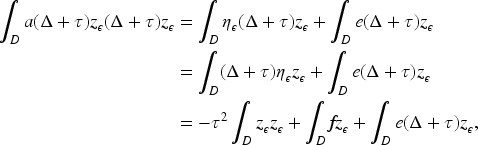
Using the equations for $θ_{ϵ}^{(2)}$ and $w_{ϵ}$ and the second Green’s identity twice, we obtain
$\begin{aligned} \int_{D} θ_{ϵ}^{(2)} f & = \int_{D} [(Δ_{x} + τ) a (x / ϵ) (Δ + τ) w_{ϵ} + τ^{2} w_{ϵ}] θ_{ϵ}^{(2)} d x \\ = \int_{\partial D} θ_{ϵ}^{(2)} \frac{\partial}{\partial ν} (a (x / ϵ) (Δ + τ) w_{ϵ}) - a (x / ϵ) (Δ + τ) w_{ϵ} \frac{\partial θ_{ϵ}^{(2)}}{\partial ν} d s . \end{aligned}$
(63)
The boundary conditions for $θ_{ϵ}^{(2)}$ then yield
$\begin{aligned} \int_{D} θ_{ϵ}^{(2)} f & = \int_{\partial D} ϵ χ (x / ϵ) (Δ + τ) u_{0} \frac{\partial}{\partial ν} (a (x / ϵ) (Δ + τ) w_{ϵ}) \\ - \int_{\partial D} ϵ a (x / ϵ) (Δ + τ) w_{ϵ} \frac{\partial}{\partial ν} (χ (x / ϵ) (Δ + τ) u_{0}) d s . \end{aligned}$
(64)
From Proposition 1 applied to the homogenization problem for $w_{ϵ}$ , we found that
$\begin{aligned} ‖ w_{ϵ} - w_{0} - ϵ^{2} w^{(2)} - ϵ θ_{ϵ}^{f} ‖_{H^{2} (D)} \leq C ϵ ‖ w_{0} ‖_{H^{4} (D)}, \end{aligned}$
(65)
where $w_{0}$ is the homogenized solution for (61), $w^{(2)}$ is the corresponding bulk correction, and $θ_{ϵ}^{f}$ is its corresponding boundary corrector (for order $n = 2$ ). From line (53) in the proof of the same proposition, we have that $η_{ϵ}$ is $O (ϵ)$ in $L^{2}$ . Likewise, $Δ η_{ϵ}$ is also bounded by the same right-hand side in $L^{2} (D)$ from (54). Hence, we have that
$\begin{aligned} ‖ η_{ϵ} ‖_{L^{2} (D, Δ)} \leq C ϵ ‖ w_{0} ‖_{H^{4} (D)}, \end{aligned}$
where we use the space (see, e.g., Valli, 2023)
$\begin{aligned} L^{2} (D, Δ) = {v \in L^{2} (D) | Δ v \in L^{2} (D)} \end{aligned}$
with norm
$\begin{aligned} ‖ v ‖_{L^{2} (D, Δ)} = ‖ v ‖_{L^{2} (D)} + ‖ Δ v ‖_{L^{2} (D)} . \end{aligned}$
It is known (see Appendix A.2) that $L^{2} (D, Δ)$ has bounded boundary traces in $H^{- 1 / 2}$ and bounded normal derivative boundary traces in $H^{- 3 / 2}$ . From this and the proof of Proposition 1, we can conclude that
$\begin{aligned} ‖ a (Δ + τ) w_{ϵ} - {\bar{a^{- 1}}}^{- 1} (Δ + τ) w_{0} - ϵ a (Δ + τ) θ_{ϵ}^{f} ‖_{H^{- 1 / 2} (\partial D)} \leq C ϵ ‖ w_{0} ‖_{H^{4} (D)} \end{aligned}$
(66)
and
$\begin{aligned} {‖ \frac{\partial}{\partial ν} (a (Δ + τ) w_{ϵ}) - {\bar{a^{- 1}}}^{- 1} \frac{\partial}{\partial ν} (Δ + τ) w_{0} - ϵ \frac{\partial}{\partial ν} (a (Δ + τ) θ_{ϵ}^{f}) ‖}_{H^{- 3 / 2} (\partial D)} \leq C ϵ ‖ w_{0} ‖_{H^{4} (D)} . \end{aligned}$
(67)
Thanks to these estimates, we can replace the $w_{ϵ}$ terms in (64), with the remainder bounded by
$\begin{aligned} C ϵ^{2} ‖ χ (x / ϵ) (Δ + τ) u_{0} ‖_{H^{3 / 2} (\partial D)} ‖ w_{0} ‖_{H^{4} (D)} \end{aligned}$
for the first term and
$\begin{aligned} C ϵ^{2} ‖ \frac{\partial}{\partial ν} χ (x / ϵ) (Δ + τ) u_{0} ‖_{H^{1 / 2} (\partial D)} ‖ w_{0} ‖_{H^{4} (D)}, \end{aligned}$
for the second term. Both of these are bounded by $C ϵ^{1 / 2} ‖ u_{0} ‖_{H^{4} (D)} ‖ w_{0} ‖_{H^{4} (D)}$ , where we abuse notation and continue to use $C$ for the constant. Since we have assumed that $D$ is smooth, we use the standard elliptic estimate that
$\begin{aligned} ‖ w_{0} ‖_{H^{4} (D)} \leq C ‖ f ‖_{L^{2} (D)}, \end{aligned}$
so the remainder is bounded by $C ϵ^{1 / 2} ‖ f ‖_{L^{2} (D)} ‖ u_{0} ‖_{H^{4} (D)}$ . Hence (64) becomes
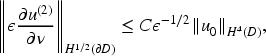
$\begin{aligned} \int_{D} θ_{ϵ}^{(2)} f & = \int_{\partial D} ϵ χ (x / ϵ) (Δ + τ) u_{0} \frac{\partial}{\partial ν} ({\bar{a^{- 1}}}^{- 1} (Δ + τ) w_{0}) d s \\ \times \int_{\partial D} ϵ^{2} χ (x / ϵ) (Δ + τ) u_{0} \frac{\partial}{\partial ν} (a (x / ϵ) (Δ + τ) θ_{ϵ}^{f}) d s \\ - \int_{\partial D} ϵ {\bar{a^{- 1}}}^{- 1} (Δ + τ) w_{0} \frac{\partial}{\partial ν} (χ (x / ϵ) (Δ + τ) u_{0}) d s \\ - \int_{\partial D} ϵ^{2} a (x / ϵ) (Δ + τ) θ_{ϵ}^{f} \frac{\partial}{\partial ν} (χ (x / ϵ) (Δ + τ) u_{0}) d s + o (1) \\ = I + I I + I I I + I V + o (1), \end{aligned}$
(68)
where the tail is bounded in absolute value by $C ϵ^{1 / 2} ‖ f ‖_{L^{2} (D)} ‖ u_{0} ‖_{H^{4} (D)}$ . The first term $I$ is clearly bounded by the same, as it in fact goes to zero $O (ϵ)$ . For the third term $I I I$ , the normal derivative produces a $1 / ϵ$ when applied to $χ$ , which cancels with the $ϵ$ , yielding that the absolute value of $I I I$ is bounded by $C ‖ f ‖_{L^{2} (D)} ‖ u_{0} ‖_{H^{4} (D)}$ . For the other two terms, we note that $a (x / ϵ) (Δ + τ) θ_{ϵ}^{f}$ is bounded by $C ϵ^{- 1 / 2} ‖ w_{0} ‖_{H^{4} (D)}$ in $L^{2} (D, Δ)$ by Corollary 1 and the equation for $θ_{ϵ}^{f}$ . Hence, we have by trace estimates for $L^{2} (D, Δ)$ (see, e.g., Appendix A.2) that
$\begin{aligned} ‖ a (x / ϵ) (Δ + τ) θ_{ϵ}^{f} ‖_{H^{- 1 / 2} (\partial D)} \leq C ϵ^{- 1 / 2} ‖ f ‖_{L^{2} (D)} \end{aligned}$
and
$\begin{aligned} ‖ \frac{\partial}{\partial ν} a (x / ϵ) (Δ + τ) θ_{ϵ}^{f} ‖_{H^{- 3 / 2} (\partial D)} \leq C ϵ^{- 1 / 2} ‖ f ‖_{L^{2} (D)} . \end{aligned}$
Using the duality pairing,
$\begin{aligned} | I I | & \leq ϵ^{2} ‖ χ (Δ + τ) u_{0} ‖_{H^{3 / 2} (\partial D)} ‖ \frac{\partial}{\partial ν} a (x / ϵ) (Δ + τ) θ_{ϵ}^{f} ‖_{H^{- 3 / 2} (\partial D)} \\ \leq C ϵ^{2} ϵ^{- 3 / 2} ‖ u_{0} ‖_{H^{4} (D)} ϵ^{- 1 / 2} ‖ f ‖_{L^{2} (D)} \end{aligned}$
(69)
and
$\begin{aligned} | I V | & \leq ϵ^{2} ‖ \frac{\partial}{\partial ν} χ (Δ + τ) u_{0} ‖_{H^{1 / 2} (\partial D)} ‖ a (x / ϵ) (Δ + τ) θ_{ϵ}^{f} ‖_{H^{- 1 / 2} (\partial D)} \\ \leq C ϵ^{2} ϵ^{- 3 / 2} ‖ u_{0} ‖_{H^{4} (D)} ϵ^{- 1 / 2} ‖ f ‖_{L^{2} (D)}, \end{aligned}$
(70)
from which we can conclude that
$\begin{aligned} | \int_{D} θ_{ϵ}^{(2)} f | \leq C ‖ u_{0} ‖_{H^{4} (D)} ‖ f ‖_{L^{2} (D)}, \end{aligned}$
from which the result follows.
Corollary 2
Let $u_{ϵ}, u_{0} \in H_{0}^{2} (D)$ be the solutions to
$\begin{aligned} (Δ_{x} + τ) a (x / ϵ) (Δ + τ) u_{ϵ} + τ^{2} u_{ϵ} = h \end{aligned}$
(71)
and
$\begin{aligned} (Δ_{x} + τ) {\bar{a^{- 1}}}^{- 1} (Δ + τ) u_{0} + τ^{2} u_{0} = h, \end{aligned}$
(72)
respectively. Then
$\begin{aligned} ‖ u_{ϵ} - (u_{0} + ϵ θ_{ϵ}^{(2)}) ‖_{L^{2} (D)} \leq C ϵ^{2} ‖ u_{0} ‖_{H^{5} (D)} \end{aligned}$
and
$\begin{aligned} ‖ u_{ϵ} - u_{0} ‖_{L^{2} (D)} \leq C ϵ ‖ u_{0} ‖_{H^{4} (D)}, \end{aligned}$
where the boundary correction $θ_{ϵ}^{(2)}$ is given by (43) with $n = 2$ .
Proof.
The first estimate follows from Proposition 2 and Lemma 2 applied to $θ_{ϵ}^{(3)}$ , and the second follows from Proposition 1 and Lemma 2 applied to $θ_{ϵ}^{(2)}$ .
4. Transmission Eigenvalue Expansions

The following result about nonlinear eigenvalue perturbations is an extension of a special case of the results in Osborn (1975). This is a slight modification of Corollary 4.1 in Moskow (2015) for the case where we assume only that the operators themselves converge pointwise (strongly), without assuming convergence of the adjoints. The necessary modifications were shown in Furia and Moskow (2025).

Theorem 1
Let $X$ be a Hilbert space with sesquilinear inner product $⟨, ⟩$ and ${T_{ϵ} (τ) : X \to X}$ be a set of compact linear operator valued functions of $τ$ , which are analytic in a region $U$ of the complex plane, such that $T_{ϵ} (τ) \to T_{0} (τ)$ pointwise as $ϵ \to 0$ uniformly for $τ \in U$ , and that ${T_{ϵ} (τ)}$ are collectively compact, uniformly in $U$ . Let $τ_{0} \neq 0$ , $τ_{0} \in U$ be a simple nonlinear eigenvalue of $T_{0}$ , define $D T_{0} (τ_{0})$ to be the derivative of $T_{0}$ with respect to $τ$ evaluated at $τ_{0}$ , and let $ϕ$ be a normalized eigenfunction. Then for any $ϵ$ small enough, there exists $τ_{ϵ}$ a simple nonlinear eigenvalue of $T_{ϵ}$ , such that if
$\begin{aligned} 1 + τ_{0}^{2} ⟨ D T_{0} (τ_{0}) ϕ, ϕ ⟩ \neq 0, \end{aligned}$
there exists a constant $C$ independent of $ϵ$ such that
$\begin{aligned} | τ_{ϵ} - (τ_{0} + \frac{τ_{0}^{2} ⟨ (T_{0} (τ_{0}) - T_{ϵ} (τ_{0})) ϕ, ϕ ⟩}{1 + τ_{0}^{2} ⟨ D T_{0} (τ_{0}) ϕ, ϕ ⟩}) | \leq C sup_{τ \in U} ‖ (T_{0} (τ) - T_{ϵ} (τ)) |_{R (E)} ‖^{2}, \end{aligned}$
(73)
where $R (E)$ is the one-dimensional eigenspace spanned by $ϕ$ .

Now, let us consider our operators
$\begin{aligned} T_{ϵ} (τ) : L^{2} (D) \to L^{2} (D), T_{ϵ} (τ) = A_{τ, ϵ}^{- 1} B, \end{aligned}$
(74)
where $A_{τ, ϵ}^{- 1} : H_{0}^{2} (D) \to H_{0}^{2} (D)$ is given by
$\begin{aligned} A_{τ, ϵ}^{- 1} f = {((Δ + τ) \frac{1}{n_{ϵ} - 1} (Δ + τ) + τ^{2})}^{- 1} Δ Δ f \end{aligned}$
and $B : L^{2} (D) \to H_{0}^{2} (D)$
$\begin{aligned} B f = (Δ Δ)^{- 1} Δ f, \end{aligned}$
so that
$\begin{aligned} T_{ϵ} (τ) f = {((Δ + τ) \frac{1}{n_{ϵ} - 1} (Δ + τ) + τ^{2})}^{- 1} Δ f \end{aligned}$
(75)
and
$\begin{aligned} T_{0} (τ) f = {((Δ + τ) \frac{1}{\bar{n} - 1} (Δ + τ) + τ^{2})}^{- 1} Δ f, \end{aligned}$
(76)
where the inverses of the fourth-order operators have range in $H_{0}^{2} (D)$ . We note that $T_{ϵ} (τ)$ and $T_{0} (τ)$ are well defined and compact on $L^{2} (D)$ . This follows because $Δ f$ makes sense in $H^{- 2} (D)$ , the dual of $H_{0}^{2} (D)$ , so that the range of both operators is in $H_{0}^{2} (D)$ , which embeds compactly in $L^{2}$ . We can therefore take $X = L^{2} (D)$ , with the usual inner product, when applying the above theorem.

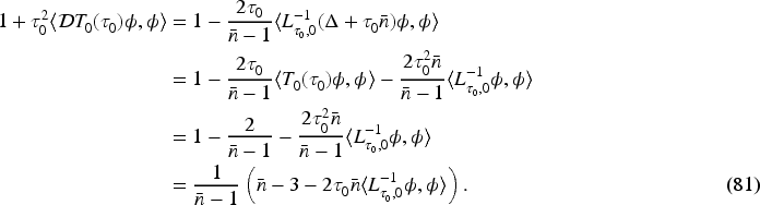
For the denominator in the correction theorem, we must compute the derivative of $T_{0} (τ)$ with respect to $τ$ , $D T_{0} (τ)$ . In fact, this derivative is computed in Cakoni, Moskow, et al. (2015), and we include the computations in Appendix A.1 for the reader’s convenience. In our case, formula (89) simplifies since our $n_{0} = \bar{n}$ is constant. In particular, the derivative $D T_{0} (τ) : L^{2} (D) \to L^{2} (D)$ is given by $D T_{0} (τ) u = - v$ , where $v \in H_{0}^{2} (D)$ solves
$\begin{aligned} Δ Δ A_{τ, 0} v = \frac{2}{\bar{n} - 1} (Δ + τ \bar{n}) A_{τ, 0}^{- 1} B u . \end{aligned}$
(77)
Note that the range of $T_{0} (τ)$ and its derivative is $H_{0}^{2} (D)$ . Next, we compute $⟨ D T_{0} (τ_{0}) ϕ, ϕ ⟩$ , where $ϕ$ is an eigenvector corresponding $τ_{0}$ . To this end, let us denote by $L_{τ, 0} : H_{0}^{2} (D) \to H^{- 2} (D)$ the mapping
$\begin{aligned} L_{τ, 0} u = ((Δ + τ) \frac{1}{\bar{n} - 1} (Δ + τ) + τ^{2}) u . \end{aligned}$
(78)
Thus, we have
$\begin{aligned} T_{0} (τ) = L_{τ, 0}^{- 1} Δ . \end{aligned}$
Note that $L_{τ, 0}$ is coercive, which means that $⟨ L_{τ, 0} u, u ⟩_{H^{- 2}, H_{0}^{2}} \geq α ‖ u ‖_{H_{0}^{2}}$ , and its inverse is well defined with range in $H_{0}^{2} (Ω)$ . Recalling also that $A_{τ_{0}, 0}^{- 1} = L_{τ, 0}^{- 1} Δ Δ$ , we have $A_{τ_{0}, 0} = (Δ Δ)^{- 1} L_{τ, 0}$ , and equation (77) becomes
$\begin{aligned} L_{τ, 0} v = \frac{2}{\bar{n} - 1} (Δ + τ \bar{n}) T_{0} (τ) u, \end{aligned}$
(79)
and hence
$\begin{aligned} D T_{0} (τ) u = - L_{τ, 0}^{- 1} \frac{2}{\bar{n} - 1} (Δ + τ \bar{n}) T_{0} (τ) u . \end{aligned}$
(80)
If we now take $τ = τ_{0}$ and $u = ϕ$ to be the $L^{2}$ -normalized homogenized transmission eigenfunction corresponding to the transmission eigenvalue $τ_{0}$ , this gives
$\begin{aligned} D T_{0} (τ_{0}) ϕ = - \frac{1}{τ_{0}} \frac{2}{\bar{n} - 1} L_{τ_{0}, 0}^{- 1} (Δ + τ_{0} \bar{n}) ϕ, \end{aligned}$
since we know that
$\begin{aligned} ϕ = τ_{0} T_{0} (τ_{0}) ϕ . \end{aligned}$
The above calculations yield
$\begin{aligned} 1 + τ_{0}^{2} ⟨ D T_{0} (τ_{0}) ϕ, ϕ ⟩ & = 1 - \frac{2 τ_{0}}{\bar{n} - 1} ⟨ L_{τ_{0}, 0}^{- 1} (Δ + τ_{0} \bar{n}) ϕ, ϕ ⟩ \\ = 1 - \frac{2 τ_{0}}{\bar{n} - 1} ⟨ T_{0} (τ_{0}) ϕ, ϕ ⟩ - \frac{2 τ_{0}^{2} \bar{n}}{\bar{n} - 1} ⟨ L_{τ_{0}, 0}^{- 1} ϕ, ϕ ⟩ \\ = 1 - \frac{2}{\bar{n} - 1} - \frac{2 τ_{0}^{2} \bar{n}}{\bar{n} - 1} ⟨ L_{τ_{0}, 0}^{- 1} ϕ, ϕ ⟩ \\ = \frac{1}{\bar{n} - 1} (\bar{n} - 3 - 2 τ_{0} \bar{n} ⟨ L_{τ_{0}, 0}^{- 1} ϕ, ϕ ⟩) . \end{aligned}$
(81)
This expression is obviously nonzero if $1 < \bar{n} \leq 3$ , since $L_{τ_{0}, 0}^{- 1}$ is nonnegative and $τ_{0} > 0$ . To compute $L_{τ_{0}, 0}^{- 1} ϕ$ for the given transmission eigenpair $(τ_{0}, ϕ)$ of the homogenized problem, one must solve
$\begin{aligned} (Δ + τ_{0}) \frac{1}{\bar{n} - 1} (Δ + τ_{0}) w + τ_{0}^{2} w = ϕ for w \in H_{0}^{2} (D) . \end{aligned}$
Thus, it is easy to numerically check if $(\bar{n} - 3 - 2 τ_{0} \bar{n} ⟨ w, ϕ ⟩) \neq 0$ . In order to evaluate the numerator, we use the asymptotic estimate developed above. To this end, we have
$\begin{aligned} T_{0} (τ_{0}) ϕ - T_{ϵ} (τ_{0}) ϕ = L_{τ_{0}, 0}^{- 1} Δ ϕ - L_{τ_{0}, ϵ}^{- 1} Δ ϕ, \end{aligned}$
where $u_{ϵ} := L_{τ_{0}, ϵ}^{- 1} Δ ϕ$ and $u_{0} := L_{τ_{0}, 0}^{- 1} Δ ϕ$ and $u_{ϵ} := L_{τ_{0}, ϵ}^{- 1} Δ ϕ$ are the solutions of
$\begin{aligned} (Δ + τ) \frac{1}{n (x / ϵ) - 1} (Δ + τ_{0}) u_{ϵ} + τ_{0}^{2} u_{ϵ} = Δ ϕ \end{aligned}$
and
$\begin{aligned} (Δ + τ) \frac{1}{\bar{n} - 1} (Δ + τ_{0}) u_{0} + τ_{0}^{2} u_{0} = Δ ϕ, \end{aligned}$
respectively. From Corollary 2, we have that
$\begin{aligned} ⟨ T_{0} (τ_{0}) ϕ - T_{ϵ} (τ_{0}) ϕ, ϕ ⟩ = - ⟨ ϵ θ_{ϵ}, ϕ ⟩ + O (ϵ^{2}), \end{aligned}$
(82)
where $θ_{ϵ}$ is the solution of
$\begin{aligned} (Δ + τ_{0}) \frac{1}{n (x / ϵ) - 1} (Δ + τ_{0}) θ_{ϵ}^{(2)} + τ_{0}^{2} θ_{ϵ}^{(2)} = 0 & in D, \\ θ_{ϵ}^{(2)} = - ϵ u^{(2)} & on \partial D, \\ \frac{\partial θ_{ϵ}^{(2)}}{\partial ν} = - ϵ \frac{\partial u^{(2)}}{\partial ν} & on \partial D, \\ with u^{(2)} = \frac{1}{τ_{0}} χ (y) (Δ_{x} + τ_{0}) ϕ χ = \frac{β}{\bar{n} - 1}, \end{aligned}$
(83)
where $β$ is $Y$ -periodic, has cell average zero, and solves
$\begin{aligned} Δ_{y} β (y) = n (y) - \bar{n}, \end{aligned}$
where we used that $u_{0} = ϕ / τ_{0}$ .
Theorem 2
Assume $n_{ϵ} := n (x / ϵ) \in L^{\infty} (D)$ is periodic in $y := x / ϵ$ for $y \in Y = [0, 1]^{d}$ , and $n (y) - 1$ is positive uniformly in $Y$ . Let $τ_{0}$ be a simple transmission eigenvalue of the homogenized problem with constant refractive index $\bar{n}$ , and $ϕ$ the corresponding eigenfunction normalized such that $‖ ϕ ‖_{L^{2} (D)} = 1$ . We assume that $\partial D$ is smooth enough so that $ϕ \in H^{5} (D)$ . Then for any $ϵ > 0$ sufficiently small, there exists a simple transmission eigenvalue $τ_{ϵ} > 0$ of the periodic media with refractive index $n (x / ϵ)$ , which satisfies the following asymptotic expansion:
$\begin{aligned} τ_{ϵ} = τ_{0} + ϵ \frac{τ_{0}^{2} (1 - \bar{n}) {⟨ θ_{ϵ}^{(2)}, ϕ ⟩}_{L^{2} (D)}}{\bar{n} - 3 - 2 τ_{0} \bar{n} ⟨ L_{τ_{0}, 0}^{- 1} ϕ, ϕ ⟩_{L^{2} (D)}} + O (ϵ^{2}) \end{aligned}$
(84)
provided that $⟨ L_{τ_{0}, 0}^{- 1} ϕ, ϕ ⟩_{L^{2} (D)} \neq (\bar{n} - 3) / (2 τ_{0} \bar{n})$ , where $θ_{ϵ}^{(2)}$ is given by (83) and $L_{τ_{0}, 0}$ is given by (78).
Proof.
First, we note that Corollary 2 gives us that for any given $f \in L^{2} (Ω)$ ,
$\begin{aligned} ‖ (T_{ϵ} (τ) - T_{0} (τ)) f ‖_{L^{2} (Ω)} \leq C_{τ} ϵ . \end{aligned}$
(85)
For $τ$ given in a bounded region of the complex plane, $C_{τ}$ can be bounded independently of $τ$ from the explicit coercivity of the fourth-order operator (Cakoni & Haddar, 2009). Hence, we have strong pointwise convergence of the operators in $L^{2} (Ω)$ . Furthermore, the operators ${T_{ϵ} (τ)}$ are collectively compact, since ${u_{ϵ} = T_{ϵ} (τ) f}$ satisfy
$\begin{aligned} ‖ u_{ϵ} ‖_{H^{2} (Ω)} \leq C ‖ f ‖_{L^{2} (Ω)}, \end{aligned}$
where $C$ is independent of $ϵ$ and $τ$ . Hence, we can apply Theorem 1. Furthermore, (85) says that the right-hand side of (73) is $O (ϵ^{2})$ , since the eigenspace $R (E)$ is finite dimensional (in fact one-dimensional in our case). We have already calculated the expressions on the left-hand side of (73); the denominator is given by (81) and the numerator is given by (82). The result follows from inserting these formulas into (73).
Remark 3
It would be desirable to have the correction value in formula (88) be independent of $ϵ$ . Note that from Lemma 2, we have that the term $⟨ θ_{ϵ}^{(2)}, ϕ ⟩$ is bounded with respect to $ϵ$ , so any sequence of $ϵ_{k} \to 0$ will have subsequential limits. We would like to characterize its limit points, or at least rewrite it in a more explicit form. For similar eigenvalue problems in second-order homogenization in bounded domains (Gérard-Varet & Masmoudi, 2011, 2012; Moskow & Vogelius, 1997a, 1997b; Santosa & Vogelius, 1993), the precise value of the boundary corrector limit is complicated by two factors: (i) The limit may not be unique if the domain has a boundary with flat parts of rational or infinite slope. We expect that the limit will be unique for smooth $D$ in which the boundary has no flat parts. (ii) Even when the limit is unique, there is no known explicit characterization of the limit. It may very well be the case that the first-order transmission eigenvalue corrections exhibit both of these complications. One needs to study the behavior of the boundary correctors for fourth-order homogenization problems, and this is the subject of future work. In the next section, we consider the one-dimensional case, which is easier to analyze, and demonstrates that the corrector is not generically zero. Furthermore, if the scatterer has flat parts with rational or infinite slope, the one-dimensional study suggests that the corrector will depend on how the boundary cuts the microstructure.
5. The One-Dimensional Case

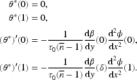
Although we explicitly took the dimension $d = 2$ or $d = 3$ , the same results clearly hold for $d = 1$ . Let us take $D = (0, 1)$ for simplicity, while noting that the following can easily be extended with small modifications to general intervals $(a, b)$ . Recalling that the eigenfunction has zero Cauchy data at the boundary, the one-dimensional boundary corrector function $θ_{ϵ}^{(2)}$ here satisfies

\begin{aligned} (\frac{d^{2}}{d x^{2}} + τ_{0}) \frac{1}{n (x / ϵ) - 1} (\frac{d^{2}}{d x^{2}} + τ_{0}) θ_{ϵ}^{(2)} + τ_{0}^{2} θ_{ϵ}^{(2)} = 0 on (0, 1), \\ θ_{ϵ}^{(2)} (0) = - ϵ \frac{β (0)}{τ_{0} (\bar{n} - 1)} \frac{d^{2} ϕ}{d x^{2}} (0), \\ θ_{ϵ}^{(2)} (1) = - ϵ \frac{β (1 / ϵ)}{τ_{0} (\bar{n} - 1)} \frac{d^{2} ϕ}{d x^{2}} (1), \\ (θ_{ϵ}^{(2)})^{'} (0) = - \frac{1}{τ_{0} (\bar{n} - 1)} \frac{d β}{d y} (0) \frac{d^{2} ϕ}{d x^{2}} (0) - ϵ \frac{β (0)}{τ_{0} (\bar{n} - 1)} \frac{d^{3} ϕ}{d x^{3}} (0), \\ (θ_{ϵ}^{(2)})^{'} (1) = - \frac{1}{τ_{0} (\bar{n} - 1)} \frac{d β}{d y} (1 / ϵ) \frac{d^{2} ϕ}{d x^{2}} (1) - ϵ \frac{β (1 / ϵ)}{τ_{0} (\bar{n} - 1)} \frac{d^{3} ϕ}{d x^{3}} (1) . \end{aligned}

(86)

In the limit, the boundary terms with

ϵ

will disappear, and so the limit will be dominated by the first terms of the Neumann data. Notice that as

ϵ \to 0

, this first term is fixed on the left but changing with

ϵ

on the right. We see here that the limit of this boundary data is not unique, and depends on the sequence

ϵ_{k} \to 0

. Assume that

\begin{aligned} ϵ_{k} = \frac{1}{N_{k} + δ}, \end{aligned}

where

N_{k} \to \infty

are integers, so that

1 / ϵ_{k} - ⌊ 1 / ϵ_{k} ⌋ = δ

, and

\begin{aligned} \frac{d β}{d y} (1 / ϵ_{k}) = \frac{d β}{d y} (δ), \end{aligned}

due to periodicity. The sequences

ϵ_{k}

for which the boundary corrector has a limit are those for which this cutoff

δ_{k}

has a limit

δ

. We see that for a fixed cutoff, the equation for the corrector becomes a standard fourth-order homogenization problem. Hence, the corrector converges in

L^{2}

at order

ϵ

θ^{*}

, the solution to

\begin{aligned} (\frac{d^{2}}{d x^{2}} + τ_{0}) \frac{1}{\bar{n} - 1} (\frac{d^{2}}{d x^{2}} + τ_{0}) θ^{*} + τ_{0}^{2} θ^{*} & = 0 on (0, 1), \end{aligned}

(87)

\begin{aligned} θ^{*} (0) & = 0, \\ θ^{*} (1) & = 0, \\ (θ^{*})^{'} (0) & = - \frac{1}{τ_{0} (\bar{n} - 1)} \frac{d β}{d y} (0) \frac{d^{2} ϕ}{d x^{2}} (0), \\ (θ^{*})^{'} (1) & = - \frac{1}{τ_{0} (\bar{n} - 1)} \frac{d β}{d y} (δ) \frac{d^{2} ϕ}{d x^{2}} (1) . \end{aligned}

We therefore have an explicit formula for the transmission eigenvalue corrector in one dimension, summarized in the following theorem.

Theorem 3

Assume the dimension $d = 1$ with period cell $Y = [0, 1]$ , and $n_{ϵ} := n (x / ϵ) \in L^{\infty} (D)$ is periodic in $y := x / ϵ$ such that $n (y) - 1$ is positive uniformly in $Y$ . Let $τ_{0}$ be a simple transmission eigenvalue of the homogenized problem with constant refractive index $\bar{n}$ , and $ϕ$ the corresponding eigenfunction normalized such that $‖ ϕ ‖_{L^{2} (D)} = 1$ . Assume

\begin{aligned} ϵ_{k} = \frac{1}{N_{k} + δ}, \end{aligned}

where

N_{k} \to \infty

are integers. Then, for any

k

sufficiently large, there exists a simple transmission eigenvalue

τ_{ϵ} > 0

of the periodic media with refractive index

n (x / ϵ)

, which satisfies the following asymptotic expansion:

\begin{aligned} τ_{ϵ} = τ_{0} + ϵ \frac{τ_{0}^{2} (1 - \bar{n}) {⟨ θ^{*}, ϕ ⟩}_{L^{2} (D)}}{\bar{n} - 3 - 2 τ_{0} \bar{n} ⟨ L_{τ_{0}, 0}^{- 1} ϕ, ϕ ⟩_{L^{2} (D)}} + O (ϵ^{2}) \end{aligned}

(88)

provided that

⟨ L_{τ_{0}, 0}^{- 1} ϕ, ϕ ⟩_{L^{2} (D)} \neq (\bar{n} - 3) / (2 τ_{0} \bar{n})

, where

θ^{*}

is given by (87) and

L_{τ_{0}, 0}

is given by (78).

6. Conclusions

In this article, we derived an asymptotic expansion for the transmission eigenvalues of a scatterer with periodically varying index of refraction in the case when the contrast does not change sign. In this situation, we were able to use the fourth-order formulation for the transmission eigenvalue problem, and its analysis required us to study a fourth-order homogenization problem. The two-scale asymptotics reveal a boundary corrector as the largest microstructure effect, and this boundary corrector appears in the correction formula for the transmission eigenvalues. It appears that this boundary corrector function may exhibit all of the difficulties of the boundary correctors in many second-order homogenization problems; in particular, the lack of an explicit formula for its limit for dimension $d \geq 2$ , even in the case of smooth domains. An explicit formula would allow us to determine what information about the microstructure of the medium can be extracted from the transmission eigenvalues. The analysis of these fourth-order boundary correctors is therefore of great interest, and is the subject of our future work.

Footnotes

Acknowledgments

The authors would also like to acknowledge the AIM institute and the SQuaRE program “Scattering Properties of Multiscale Heterogeneous Media,” which also supported this research.

ORCID iD

Shari Moskow

Funding

The authors disclosed receipt of the following financial support for the research, authorship, and/or publication of this article: F. Cakoni was partially supported by NSF grant no. DMS-24-06313. S. Moskow was partially supported by NSF grant nos. DMS-2008441 and DMS-2308200.

Declaration of Conflicting Interests

The authors declared no potential conflicts of interest with respect to the research, authorship, and/or publication of this article.

Appendix: Technical Lemmas

References

Cakoni

Colton

Haddar

(2010). On the determination of Dirichlet or transmission eigenvalues from far field data. Comptes Rendus de l’Académie des Sciences, Paris, 348(7–8), 379–383. https://doi.org/10.1016/j.crma.2010.02.003

Cakoni

Colton

Haddar

(2023). Inverse scattering theory and transmission eigenvalues. In CBMS-NSF regional conference series in applied mathematics (2nd ed., Vol. 98, pp. 173–184). Society for Industrial and Applied Mathematics (SIAM).

Cakoni

Gintides

Haddar

(2010). The existence of an infinite discrete set of transmission eigenvalues. SIAM Journal on Mathematical Analysis, 42(1), 237–255. https://doi.org/10.1137/090769338

Cakoni

Guzina

B. B.

Moskow

Pangburn

(2019). Scattering by a bounded highly oscillating periodic medium and the effect of boundary correctors. SIAM Journal on Applied Mathematics, 79(4), 1448–1474. https://doi.org/10.1137/19M1237089

Cakoni

Haddar

(2009). On the existence of transmission eigenvalues in an inhomogeneous medium. Applicable Analysis, 88(4), 475–493. https://doi.org/10.1080/00036810802713966

Cakoni

Haddar

Harris

(2015). Homogenization of the transmission eigenvalue problem for periodic media and application to the inverse problem. Inverse Problems and Imaging, 9(4), 1025–1049. https://doi.org/10.3934/ipi.2015.9.1025

Cakoni

Harris

Moskow

(2017). The imaging of small perturbations in an anisotropic media. Computers & Mathematics with Applications, 74(11), 2769–2783. https://doi.org/10.1016/j.camwa.2017.06.050

Cakoni

Moskow

Pangburn

(2020). Limiting boundary correctors for periodic microstructures and inverse homogenization series. Inverse Problems, 36(6), 065009.

Cakoni

Moskow

Rome

(2015). The perturbation of transmission eigenvalues for inhomogeneous media in the presence of small penetrable inclusions. Inverse Problems and Imaging, 9(3), 725–748. https://doi.org/10.3934/ipi.2015.9.725

10.

Fornerod

Nguyen

H. M.

(2023). The Weyl law of transmission eigenvalues and the completeness of generalized transmission eigenfunctions without complementing conditions. SIAM Journal on Mathematical Analysis, 55(4), 3959–3999. https://doi.org/10.1137/22M1486157

11.

Francfort

G. A.

(1992). Homogenisation of a class of fourth order equations with application to incompressible elasticity. Proceedings of the Royal Society of Edinburgh: Section A Mathematics, 120(1–2), 25–46. https://doi.org/10.1017/S0308210500014967

12.

Furia

Moskow

(2025). First order corrections to the homogenized scattering resonances for periodic scatterers. Journal of Mathematical Physics, 66(4), 16. https://doi.org/10.1063/5.0174887

13.

Gérard-Varet

Masmoudi

(2011). Homogenization in polygonal domains. Journal of the European Mathematical Society (JEMS), 13(5), 1477–1503. https://doi.org/10.4171/JEMS/286

14.

Gérard-Varet

Masmoudi

(2012). Homogenization and boundary layers. Acta Mathematica, 209(1), 133–178. https://doi.org/10.1007/s11511-012-0083-5

15.

Kirsch

(2016). A note on Sylvester’s proof of discreteness of interior transmission eigenvalues. Comptes Rendus de l’Académie des Sciences, Paris, 354(4), 377–382. https://doi.org/10.1016/j.crma.2016.01.015

16.

Kirsch

Lechleiter

(2013). The inside–outside duality for scattering problems by inhomogeneous media. Inverse Problems, 29(10), 104011. https://doi.org/10.1088/0266-5611/29/10/104011

17.

Moskow

(2015). Nonlinear eigenvalue approximation for compact operators. Journal of Mathematical Physics, 56(11), 113512. https://doi.org/10.1063/1.4936304

18.

Moskow

Vogelius

(1997a). First-order corrections to the homogenised eigenvalues of a periodic composite medium. A convergence proof. Proceedings of the Royal Society of Edinburgh Section A, 127(6), 1263–1299.

19.

Moskow

Vogelius

(1997b). First order corrections to the homogenized eigenvalues of a periodic composite medium: The case of Neumann boundary conditions. http://www.math.drexel.edu/∼moskow/

20.

Niu

Shen

(2018). Convergence rates and interior estimates in homogenization of higher order elliptic systems. Journal of Functional Analysis, 274(8), 2356–2398. https://doi.org/10.1016/j.jfa.2018.01.012

21.

Niu

(2019). Uniform boundary estimates in homogenization of higher-order elliptic systems. Annali di Matematica Pura ed Applicata (4), 198(1), 97–128. https://doi.org/10.1007/s10231-018-0764-6

22.

Osborn

J. E.

(1975). Spectral approximation for compact operators. Mathematics of Computation, 29, 712–725.

23.

Pastukhova

(2017). Operator error estimates for homogenization of fourth order elliptic equations. St. Petersburg Mathematical Journal, 28(2), 273–289. https://doi.org/10.1090/spmj/1450

24.

Robbiano

(2013). Spectral analysis of the interior transmission eigenvalue problem. Inverse Problems, 29(10), 104014. https://doi.org/10.1088/0266-5611/29/10/104001

25.

Santosa

Vogelius

(1993). First-order corrections to the homogenized eigenvalues of a periodic composite medium. SIAM Journal on Applied Mathematics, 53(6), 1636–1668. https://doi.org/10.1137/0153076

26.

Valli

(2023). A well-posed variational formulation of the Neumann boundary value problem for the biharmonic operator. https://arxiv.org/abs/2306.00776

27.

Vodev

(2018). High-frequency approximation of the interior Dirichlet-to-Neumann map and applications to the transmission eigenvalues. Analysis of Partial Differential Equations, 11(1), 213–236. https://doi.org/10.2140/apde.2018.11.213

28.

Vodev

(2025). Interior transmission problems with coefficients of low regularity. Inverse Problems and Imaging, 19(1), 1–33. https://doi.org/10.3934/ipi.2024023