Linear and quadratic utility loss functions in voting behavior research

Abstract

Numerous studies examine voting behavior based on the formal theoretical predictions of the spatial utility model. These studies model individual utility from the election of a preferred party or candidate as decreasing as the alternative deviates from one’s ideal point, but differ as to whether this loss should be modeled linearly or quadratically. After advancing a theoretical argument for linear loss, this paper uses a wealth of data across 20 countries to empirically examine the predictive power of these two loss functions in terms of both voter choice and voter turnout. Results indicate that the linear loss function outperforms the quadratic loss function. The findings have important implications for theoretical scholars seeking to model voter behavior, for observational scholars, who must assign utility values across parties to individuals under study, and for experimental researchers, who must entice individuals with particular utility loss functions.

Keywords

loss functions party behavior proximity voting utility voter behavior

The spatial proximity model of voter utility, most famously articulated by Anthony Downs (1957), has weathered numerous theoretical and empirical tests (see, for example, Blais et al., 2001; Gilljam, 1997; Krämer and Rattinger, 1997; Pierce, 1997; Westholm, 1997) and is the cornerstone of voting behavior research (Adams et al., 2005). In short, the model predicts that voters derive the most utility from the candidate or party closest to them on some ideological or policy continuum. As such, one is most likely to vote for the option nearest one’s ideal point, and one is more likely to vote at all when the party system provides one with an ideologically close option.

The decrease in utility associated with an alternative’s deviation from one’s ideal point is called loss, and the function that maps this loss to one’s utility value is called a loss function. Linear loss imposes a constant ‘penalty’ on deviations from one’s ideal point, while quadratic loss imposes a harsher penalty as outcomes become more and more distant. While the linear and quadratic loss functions dominate voting behavior research, decisions about which formulation to employ are generally neither made a priori, with theoretical justification, nor a posteriori, with empirical guidance, but are instead regularly made ad hoc, with little or no justification. The purpose of this paper is twofold: first, to provide theoretical guidance for which loss function voters are most likely to employ, and second, to empirically examine which functional form has more predictive power.

Determining the theoretical and empirical applicability of these functions is important for two principal reasons. First, a substantial portion of voter behavior research, whether quantitative or formal theoretical, conceives of voter utility in terms of ideal point distances. Future studies will benefit from guidance on how to best model decreasing utility as ideal points deviate. Second, much experimental research attempts to understand voter turnout and choice in the laboratory, often generating voter preferences with a particular loss function. Participants are rewarded with prizes, monetary or otherwise, for selecting the ‘best’ option. This research provides guidance for experimental researchers who seek to simulate real-world voter behavior inside the lab.

I start with a theoretical argument against quadratic loss based on its overly harsh punishment of distant alternatives. I then present an argument for linear loss based on findings from psychological research indicating that humans tend to conceive of the world in linear terms. After reviewing previous work on spatial voting, I conduct a series of examinations of voter choice and turnout using data over 30 elections and 20 countries from Modules I and II of the Comparative Study of Electoral Systems (CSES). This broad analysis allows me to test the relative performance of each loss function across a broad range of countries, providing variation in cultural and institutional constructs.

From the tests, I reach three main conclusions. First, the prevalence of proximity behavior varies widely across countries, and both observational researchers and experimentalists, regardless of particular subfield, should be aware that contextual factors have the potential to influence the usefulness of the proximity model. Second, the linear loss function is shown to better model voter utility in regard to vote choice than the quadratic loss function. Third, linear loss also outperforms quadratic loss in regard to voter turnout, though the difference is less pronounced. As assigning utility values based on linear loss better captures intuition (Ordeshook, 1986), it is not advisable to deviate from the model without a proven alternative. I suggest that both experimental and empirical researchers formulate utility based on linear loss functions in the absence of compelling evidence to do otherwise.

1. Linear and quadratic loss

Voting behavior is often modeled in terms of the physical distance between the individual and the objects in the choice set. As noted by Olson and Gale (1968: 231), ‘The minimization of physical distance is only a theoretical notion intended to simplify the formulation of abstract concepts.’ Thus, the dimension or dimensions along which such physical distances exist are not strictly observable.

In voting behavior research, such dimensions are generally thought to represent an ideological structure, and it is established that the vote decision process is well represented with ideological distances (see, for example, Blais et al., 2001; Gilljam, 1997; Krämer and Rattinger, 1997; Pierce, 1997; Westholm, 1997). As per Downs (1957), ideologies exist because voters are not informed about the policy stances of all parties. As obtaining full information about the range of party positions is likely prohibitive, ideologies are used as a cost-saving mechanism. Individuals rely on ideology as a tool to organize a complicated political world.

Spatial proximity models of voter behavior conceptualize individual utility over a particular alternative as maximized when the location of that alternative is identical to an individual’s ideological ideal point. Utility decreases, at either a constant or a changing rate, as the distance between the alternative and the individual’s ideal point increases. That is, each voter’s preference curves are single-peaked and slope downward monotonically from the point of highest utility.

Nearly all voting behavior research in the spatial proximity tradition conceptualizes the monotonic utility decrease as linear or quadratic.¹ Linear loss implies that as ideological distance increases, utility decreases at a uniform rate; a shift from a deviation of zero units to one unit will affect utility the same as a shift from a deviation of two units to three units. Quadratic loss, on the other hand, ‘penalizes’ distant alternatives (those beyond one unit) at an increasing rate by squaring the deviations from one’s ideal point. For example, a shift from a deviation of zero to a deviation of one unit will still register as a loss of ‘1’, while a shift from a deviation of two units to three units will register as a loss of ‘5’ (3² –2² = 5).

While both loss functions can be generalized to multiple dimensions, for simplicity I focus on the unidimensional case here. Equations (1) and (2) depict linear and quadratic loss respectively, each modeling the utility voter i would receive from the election of party j. As is clear from the equations and Figure 1, both functions indicate a monotonic decrease in utility as the distance from the ideal point of zero increases. The quadratic loss function provides that utility decreases at an increasing rate as this distance increases, while the linear loss function provides for a constant decrease. Note that in the positive and negative unit intervals, and only in these intervals, the linear loss function places a larger penalty on more distant alternatives than the quadratic loss function.

Linear loss: u_{ij} = - | v_{i} - p_{j} |

(1)

Quadratic loss: u_{ij} = - {(v_{i} - p_{j})}^{2}

(2)

Figure 1.

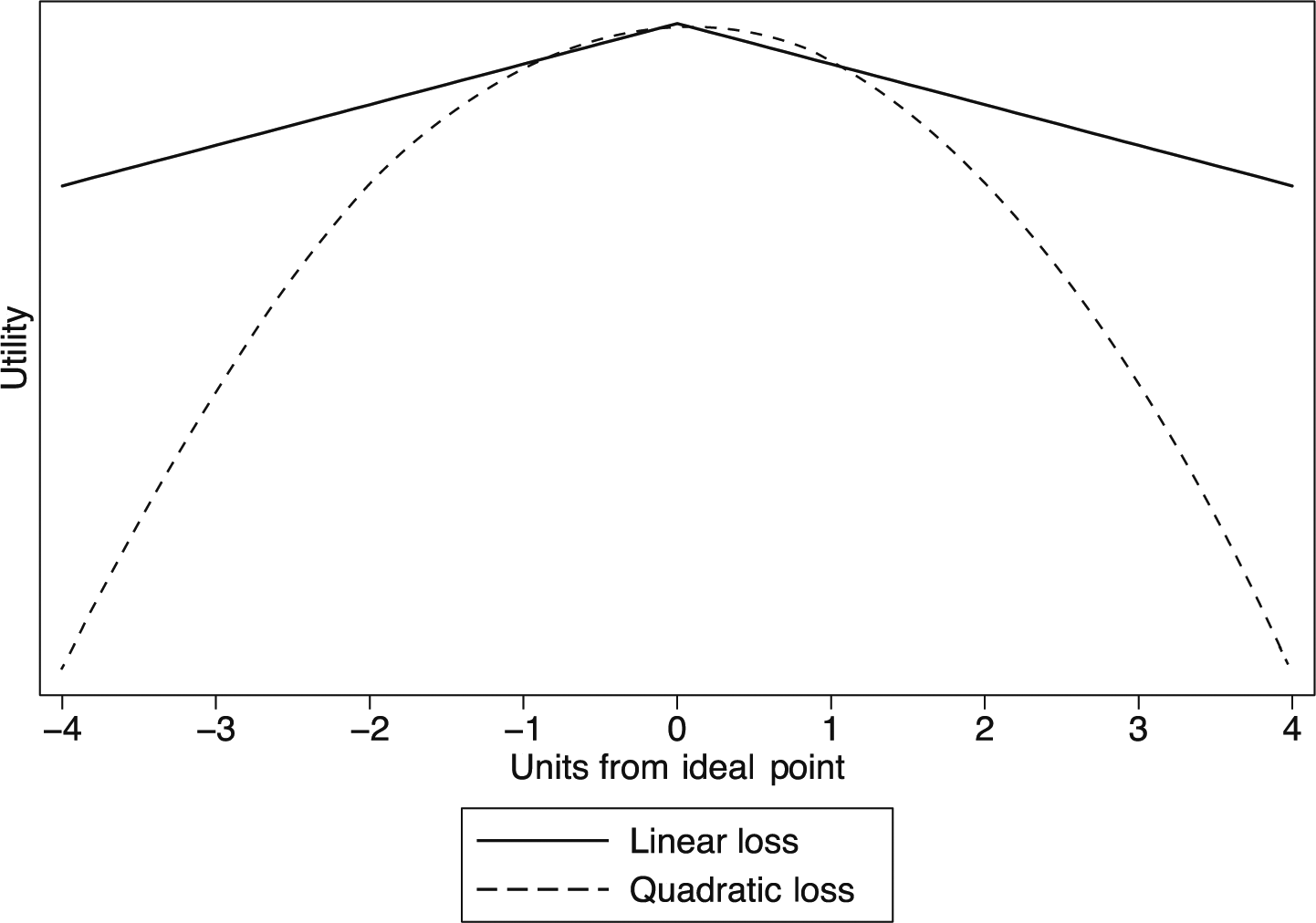
Linear and quadratic loss functions.

These loss functions clearly offer divergent conceptualizations of voter utility. The most obvious difference is in their respective treatments of distant alternatives, with the quadratic loss function assuming utility decreases dramatically as the distance between an individual’s ideal point and that of an alternative increases. Which of these two formulations best represents the process of voting, and which is thus best suited to reproduce the outcome of a voter’s decision-making process?

2. A theory of utility: which loss function is best?

The linear and quadratic conceptualizations of utility loss offer very different views of the vote decision calculus, and when one chooses between the two, one makes some strong assumptions about how voters think and behave. One crucial assumption concerns the effect of alienation on voter behavior. The alienation thesis (e.g. Adams et al., 2005; Converse, 1966; Downs, 1957; Enelow and Hinich, 1984a, 1984b; Riker and Ordeshook, 1973) predicts that individuals avoid choosing an alternative when it provides little absolute utility, irrespective of the alternative’s position in relation to its competitors (relative utility). That is, regardless of whether a particular party or candidate best represents an individual’s ideological position, if that choice provides low absolute utility, individuals will prefer to stay home. Alienated individuals are less likely to vote, and, among those who do turn out, are more likely to deviate from their first preference (Brody and Page, 1973). The psychological benefit of supporting a particular candidate is low when absolute utility is low.

Because utility drops sharply under quadratic loss as the distance to one’s closest alternative increases, the quadratic loss conceptualization assumes that individuals become ‘alienated’ quickly as their ideal point becomes more distant from those of the competing alternatives. The linear loss function, alternatively, while punishing distant alternatives, does not do so at such a sharp rate. Thus, the quadratic loss formulation implies that alienation is a very strong predictor of voter behavior, while the linear loss formulation assumes a less drastic effect of alienation.

Though Brody and Page (1973) do find empirical support for the alienation thesis, the alienation effect is not well established in other studies. In fact, most empirical work finds a null or inconsistent effect of alienation on voter turnout and choice (e.g. Guttman et al., 1994; Peress, 2011; Thurner and Eymann, 2000; Weisberg and Grofman, 1981). And, where an effect is found, it is not large. Plane and Gershtenson (2004), for example, show that the predicted difference in turnout between alienated and non-alienated individuals is just three percentage points.

Thus, it is likely that the quadratic loss function penalizes distant alternatives too harshly.² In terms of voter turnout, the use of the quadratic loss function may inflate the number of individuals considered to be alienated, thus inaccurately predicting abstention. In terms of vote choice, quadratic loss will place an extremely high premium on ideological closeness and, equivalently, a strong penalty on ideological gaps. This likely unrealistic utility structure may deflate the explanatory power of the spatial element of a vote choice³ equation. Thus, the linear loss function, which does not place such a premium on alienation, forms a more realistic utility model.

Moreover, research in psychology demonstrates that linear models powerfully capture human behavior. For example, research on inductive inference shows that individuals are better able to predict a criterion with a set of cues when the cues are linearly, rather than quadratically, related to the criterion (Brehmer, 1987). This is especially true when the amount of cueing information provided is low (Hammond and Summers, 1965). In addition, when predicting individuals’ decisions among competing tasks or objects based on a series of inputs, linear models of such inputs are shown to have robust predictive power (Dawes and Corrigan, 1974). As noted by Hastie and Dawes (2010: 60), ‘the mind is in many essential respects a linear weighting and adding device.’

Linear loss is the simplest and, in line with the aforementioned psychological research, the most reasonable functional form to assign to human utility maximization. In addition, an argument for linear loss can be made with an appeal to the scientific criterion of parsimony; there is no reason to assume non-linear loss unless there is reason to believe that doing so will increase explanatory power. Following Ordeshook (1986), then, the onus is to demonstrate that some non-linear loss function better represents voter behavior. By far the most prevalent non-linear loss function in the voting behavior canon is the quadratic formulation. I next present a non-exhaustive but extensive review of existing non-observational, observational, and experimental research employing linear and quadratic loss functions. I then test the predictive power of each formulation.

3. Theoretical voting research with loss functions

Anthony Downs’ work on voter and party behavior is well known for introducing spatial utility into political science research (1957). In his seminal work, he put forth that voters prefer the ideologically nearest party and are most likely to turn out when the party system provides them with a nearby alternative (and when they are not indifferent between alternatives). Downs also showed that candidates, whom he assumed to care only about winning elections, converge at the center in two-party elections due to their understanding of voter utility functions.

Downs’ postulates are based on the work of Hotelling (1929), who introduced the spatial utility model in terms of store locations on a street populated by evenly spread customers. As each customer will choose the nearest store, that which minimizes the distance he or she must travel, the optimal location for any given store is at the midpoint of the street. The theory of both Downs and Hotelling employs a linear loss function.

Much future theoretical research on turnout and vote choice (and party behavior as a function of vote seeking) followed the Hotelling/Downs example of operationalizing utility with a linear loss function. For example, Wittman (1973) modifies Downs’ work, assuming that parties care about winning only as a means to produce policy, but like Downs assumes that parties respond to voters whose utility is dependent upon linear loss functions. In later work, Wittman (2007) again conceptualizes loss as linear when incorporating pressure group interests into his vote choice model. In addition, Lin et al. (1999) examine equilibrium candidate competition under probabilistic voting with a linear loss function. In regard to turnout, Adams and Merrill (2003) rely on a linear loss function in presenting a model of American elections.

Alternatively, in their book-length treatment of party positioning and voter behavior, Adams et al. (2005) rely on a quadratic loss function when assigning utility over alternatives. In addition, Davis et al. (1970) explicitly expand Downs’ treatment into two dimensions, but unlike Downs assume a quadratic loss function. Enelow and Hinich (1981) develop a quadratic loss model that incorporates voter uncertainty, representing voter preferences as distributions rather than ideal points along a policy dimension. They later modify the proximity model to incorporate a set of psychological variables, again with a quadratic loss function (Enelow and Hinich, 1982). Finally, they formulate a ‘general distance representation of voter utility’ that need not make any ‘restrictive assumptions’ (Enelow and Hinich, 1984a).

Also taking an agnostic approach to the formulation of utility, Riker and Ordeshook (1968) greatly expand upon Downs’ treatment of voter turnout, but do not specify a utility function beyond indicating the usual monotonic decrease. Other theoretical work has formulated generic loss functions that assume neither a quadratic nor linear form in the search for equilibria in voter behavior and candidate positions (e.g., McKelvey and Wendell, 1976; Merrill and Adams, 2001). Such flexible representations of the loss function are perhaps ideal, but empiricists, alas, generally must choose a single function when assigning utility values to voters across alternatives.

4. Observational voting research with loss functions

Westholm (1997) argues that modeling utility as a quadratic function of distance is appropriate only if quadratic loss can be shown to fit the data as well as or better than linear loss. Still, many empirical studies employ the quadratic loss formulation. For example, Shapiro (1969) applies a model based on a quadratic loss function to data on 201 survey respondents, finding that the quadratic loss function equations correctly predict the vote intentions of 85.5% of the sample. Bartels (1986) tests Enelow and Hinich’s (1981) quadratic loss model with data from the 1980 US presidential election, finding that squared distances on eight issues negatively correlate with vote choice. Kedar (2005) employs a quadratic loss function to examine voting behavior in anticipation of coalition governments, but conducts robustness checks that employ linear loss, finding substantively inconsequential differences between the two. Duch et al. (2010) also examine coalition-directed voting with quadratic loss functions. Adams et al. (2006) use quadratic loss functions to examine whether indifference among candidates suppresses turnout, as put forth by Downs, finding support for this proposition. Jessee (2009, 2010) uses a quadratic loss formulation to examine vote choice in the 2004 and 2008 US presidential elections and shows that the model performs well among the highly informed. In a study of party positioning strategies in response to voter utility functions, Calvo and Hellwig (2011) also employ a quadratic loss formulation.

A host of other studies employ the simpler linear loss function. For example, Abramowitz (1980), using a linear loss function, finds voting in the US Senate to be highly dependent on ideological distance for independents and non-incumbent voters. Blais et al. (2001) and Krämer and Rattinger (1997) demonstrate that voter utility values based on linear loss functions strongly predict preferences over parties in Canada and in the US and Germany, respectively. Wessels and Schmitt (2008) employ a linear loss function to examine proximity behavior across 31 countries, finding linear distance to positively relate to vote choice, especially when the voter has numerous and distinct parties from which to chose. Finally, Singh (2011) employs linear loss functions, showing that the decision to turn out is a function of both a voter’s distance from his or her preferred party and electoral rules.

5. Experimental voting research with loss functions

The theory of proximity voting has also been used to inform the design of several laboratory experiments on voting behavior. Specifically, experimental researchers often attempt to entice voters to pick a given candidate or party with a certain reward, and this reward is based on the distance between the voter and the selected alternative. It is up to the researcher to decide whether such enticements should be based upon a linear loss function or a quadratic loss function. Of course, to boost external validity, experimental researchers will wish to employ the loss function that best approximates political reality.

McKelvey and Ordeshook (1985), for example, employ a linear loss function to assign utility values to participants in their laboratory study of elections under asymmetric information. Similarly, Lupia (1994) assigns linearly formulated utility values to respondents in his experimental study of certain and uncertain voters. Williams (1994), in his laboratory examination of spatial voting, calculates payoffs using a linear loss function, and provides an additional reward to participants who vote for the nearest candidate. Recently, in an experiment on strategic voting in one-and two-round elections, Blais et al. (2011) use a linear loss function to reward participants, assigning individuals to a random location on a single dimension and calculating payoffs based on the distance between the victorious candidate’s position and their own. Morton (1993), alternatively, uses a quadratic loss function to determine payments in an experimental study of candidate positioning.

Payoffs based on linear loss are most prevalent in experimental settings, likely because of the ease with which they are understood. Indeed, Ordeshook (1986: 22–23) notes that the linear loss function ‘nicely summarizes the intuition that, when comparing candidates, voters look separately at how different each is from their most preferred position on each election issue.’ Nevertheless, the usefulness of the linear loss function is only valid if it truly captures voter behavior outside of the lab.

6. Empirical tests of linear and quadratic loss

Despite the extensive amount of positive, observational, and experimental research examining voter behavior via utility functions based on either linear or quadratic loss, there has been no large-scale inquiry as to which operationalization best captures true voter behavior across countries.⁴ I gather data on individual-level vote choice and turnout from Modules I and II of the CSES. For comparability purposes, I restrict the sample to parliamentary countries, as voters in presidential races often choose based on personal characteristics rather than ideological considerations (Funk, 1999; Jackman, 1987; Norris, 2004). I also eliminate countries not rated ‘free’ by the Freedom House⁵ and drop countries with enforced compulsory voting.⁶ In the end, the sample consists of 30 elections across 20 countries.

Following the standard approach in behavioral research employing a spatial logic, I constrain voter and party positions to fall upon a single dimension (see Cox, 1990: 908), which can be thought of as left–right ideological ‘super dimension’ that constrains party positions over several issues (Gabel and Huber, 2000) and is known to be a good representation of politics (e.g. Bobbio, 1996; Budge et al., 2010). To operationalize individual utility based on the linear and quadratic loss functions, both party and respondent positions are required. The CSES is excellent in this regard, as it asks respondents to locate themselves at a value of 0 to 10 along a left–right continuum, with higher values indicating rightist ideology, and also gives expert-provided locations of political parties along this continuum.

I first test the two loss functions on both incumbent voting and voter turnout on the entire pooled sample. To model incumbent voting, I estimate the following logistic regression:

log (p_{inc} / (1 - p_{inc})) = α + β ({loss}_{inc})

(3)

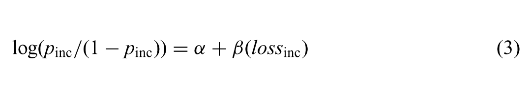
where p_inc is the probability voting for the incumbent party, loss_inc is the distance between the respondent and the incumbent party (either linear or quadratic), β is the estimated coefficient on loss_inc, and α is the estimated intercept. The necessary data are available across 38,211 individuals.

Table 1 illustrates the results of the equation estimated with voter-incumbent distances formulated with both linear and quadratic loss functions. Standard errors are clustered to correct for election-specific error variance. To compare the fit of each model, I employ Akaike’s Information Criterion (AIC) and the Bayesian Information Criterion (BIC). Lower values of the AIC and BIC indicate a better model fit.

Table 1.

Incumbent Voting, Pooled Models.

	Linear Loss		Quadratic Loss
	Coef.	z-statistic	Coef.	z-statistic
loss_inc	−0.495	−9.69	−0.102	−8.68
constant	0.194	1.67	−0.180	−2.18
AIC		42913.82		43091.15
BIC		42930.92		43108.25
Log-likelihood		−21454.91		−21543.58
Number of Observations		38211		38211
Number of Elections		30		30

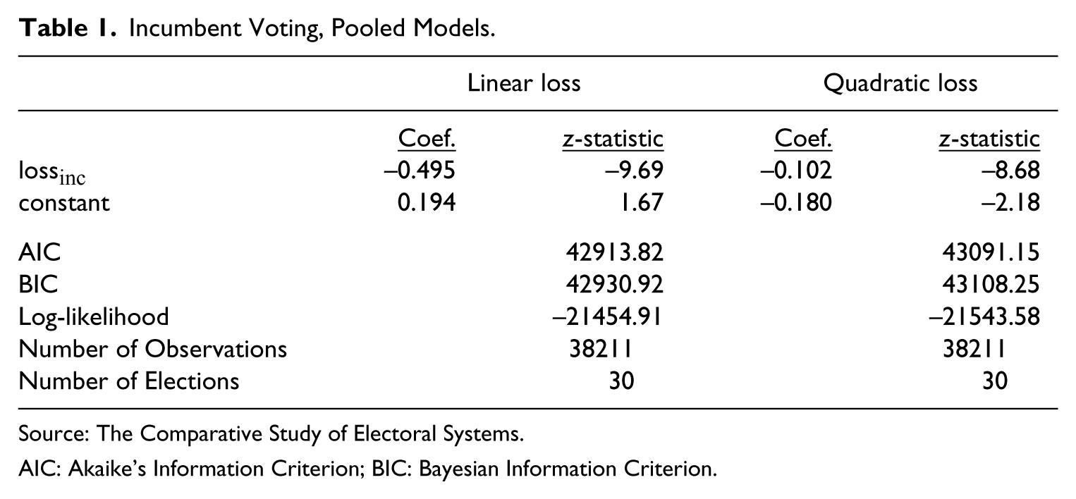
Source: The Comparative Study of Electoral Systems

AIC: Akaike’s Information Criterion; BIC: Bayesian Information Criterion.

Both estimations show that an increase in the distance between a voter’s ideal point and that of the incumbent party—or loss—decreases the likelihood one will vote for that party. Moreover, the estimated coefficient on loss_inc attains a slightly higher level of statistical significance under the linear formulation, as is apparent from the z-statistics. Note that the difference in the actual magnitudes of the estimated coefficients on loss_inc are inconsequential, as they are inherent due to the measurement differences between the two variables.

Importantly for the purposes at hand, Table 1 makes it clear that the linear loss conceptualization of voter utility provides a better model-to-data fit than the quadratic conceptualization. Both the AIC and the BIC are lower in the case of linear loss, indicating a better fit. As a rule of thumb, Burnham and Anderson (2002) note that a model with an AIC value ten units below a competing model is very likely to be the better fitting model. Further, such differences in AIC values can be used to calculate Akaike weights.⁷ Akaike weights range from 0 to 1 and are interpreted as the probability that a given model is the best-fitting model relative to the model(s) it is competing against. The Akaike weight for the linear loss specification in Table 1 is very close to 1, meaning there is a near 1.0 probability that, relative to the quadratic loss specification, it is the better-fitting model.

Next, I estimate the relative explanatory power of each conceptualization of utility in terms of voter turnout. To model turnout, I estimate the equation

log (p_{vote} / (1 - p_{vote})) = α + β ({loss}_{vote})

(4)

where p_vote is the probability voting for the incumbent party and loss_vote is the distance between the respondent and the nearest competing party (either linear or quadratic). As per the classical model of voter turnout, which incorporates the probability that one’s vote will be decisive, distances are weighted by the competitiveness of the election to which the individual is subject.⁸ β is the estimated coefficient on loss_vote and α is the estimated intercept. All else equal, one is more likely to turn out when there is an ideologically nearby party in the race (Downs, 1957; Palfrey and Rosenthal, 1983; Riker and Ordeshook, 1968). Thus, the estimates of β should be negative. The necessary data is available across 44,897 individuals, and Table 2 illustrates the estimation results.

Table 2.

Voter Turnout, Pooled Models.

	Linear loss		Quadratic loss
	Coef.	z-statistic	Coef.	z-statistic
loss_vote	−0.098	−1.20	−0.002	−0.09
Constant	1.792	10.47	1.744	10.15
AIC		37770.84		37791.86
BIC		37788.26		37809.29
Log-likelihood		−18883.42		−18893.93
Number of Observations		44897		44897
Number of Elections		30		30

Source: The Comparative Study of Electoral Systems

AIC: Akaike’s Information Criterion; BIC: Bayesian Information Criterion.

For the turnout model, both the AIC and the BIC are again lower in the case of linear loss, indicating a better model fit. In addition, Akaike weights indicate that the linear loss turnout model is the better fitting model with a probability close to 1.0. Further, the z-statistics indicate that the estimated coefficient on loss_vote has a higher level of statistical significance under the linear formulation (though neither the linear formulation nor the quadratic formulation achieves conventional levels of statistical significance).

These pooled tests provide an indicator of how well each loss function describes the data overall, but make the restrictive assumption that the coefficients on loss are identical within each election. This is likely not the case, as contextual factors can shape the usefulness of ideological criteria to voters in terms of both vote choice and turnout (Lachat, 2008; Singh, 2011; Wessels and Schmitt, 2008). Thus, to test the strength of each loss function across elections, I estimate equations (3) and (4) within each of the 30 elections, leading to a total of 60 estimations.

First, the election-by-election estimations of equation (3) are depicted in Figure 2. The figure plots the coefficient on loss_inc across each election in the sample and associated 95% confidence intervals. In terms of incumbent voting, the effect of both conceptualizations of loss are significant across an equal number of elections, and it is clear that the magnitude of these effects varies substantially across elections.

Figure 2.

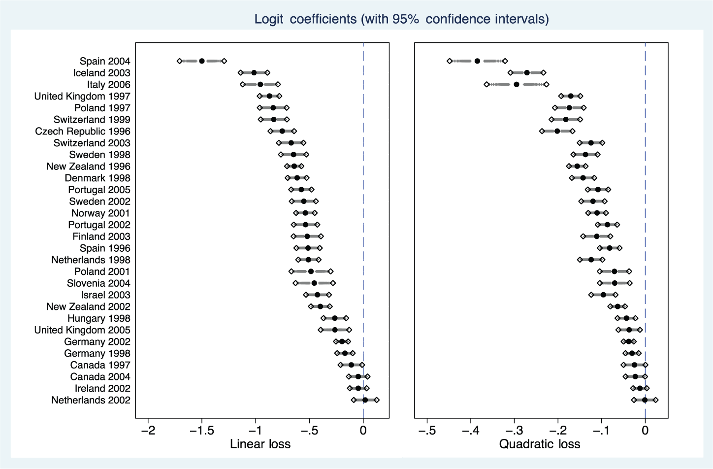
Incumbent voting across elections, linear and quadratic loss functions.

Figure 3 depicts the election-by-election estimations of equation (4), which gauges the relationship between individual-level turnout and linear or quadratic loss. As in the pooled models, loss alone is a relatively poor predictor of turnout. In fact, in certain elections it is paradoxically positively related to the probability one will vote. Again, the figure makes it clear that the effect of loss varies considerably by election, meaning a simple pooled logit model will not adequately model the data generating process.

Figure 3.

Voter turnout across elections, linear and quadratic loss functions.

To provide the most complete test of the two competing loss functions, I re-estimate equations (3) and (4) with multilevel models in which I consider individuals (level-1) to be nested within elections (level-2). I fit a unique intercept to each election and allow the coefficient on loss to vary across elections. This allows me to take full advantage of the nestedsample, while also recognizing that β in equations (3) and (4) cannot be taken as constant across elections.

Table 3 summarizes the results of the multilevel estimation of equation (3), in which the dependent variable is incumbent voting. It is clear that, on average, as the distance between an individual’s ideal point and the incumbent party increases, one is less likely to vote for that party. In addition, the z-statistics indicate that the estimated coefficient on loss_inc obtains a higher level of statistical significance under the linear formulation. Moreover, the linear formulation of loss again outperforms the quadratic formulation; the AIC and BIC statistics are both lower in the model employing linear loss, indicating a better fit. Akaike weights indicate that the model with the linear loss function is the better fitting of the two models with a probability close to 1.0.

Table 3.

Incumbent Voting, Multilevel Models.

	Linear loss		Quadratic loss
	Coef.	z-statistic	Coef.	z-statistic
loss_inc	−0.530	−9.37	−0.115	−7.77
Constant	0.256	1.80	−0.152	−7.77
Random effects parameters	Std. Dev.	z-statistic	Std. Dev.	z-statistic
loss_inc	0.304	7.39	0.080	7.21
constant	0.768	7.39	0.611	7.35
AIC		41109.62		41370.06
BIC		41143.83		41404.26
Log-likelihood		−20550.81		−20681.03
Number of Observations		38211		38211
Number of Elections		30		30

Source: The Comparative Study of Electoral Systems

AIC: Akaike’s Information Criterion; BIC: Bayesian Information Criterion.

Table 4 summarizes the results of the multilevel estimation of equation (4), in which the dependent variable is turnout. Neither formulation of loss achieves conventional levels of statistical significance, although the linear formulation is statistically more different from zero than the quadratic formulation. And again, for the turnout model, both the AIC and the BIC are lower in the case of linear loss, indicating a better fit. Further, Akaike weights again indicate that the model with the linear loss function is the better fitting of the two models with a probability close to 1.0.

Table 4.

Voter Turnout, Multilevel Models.

	Linear loss		Quadratic loss
	Coef.	z-statistic	Coef.	z-statistic
loss _vote	−0.059	−1.19	−0.013	−0.55
Constant	1.934	12.97	1.906	12.82
Random effects parameters	SD	z-statistic	SD	z-statistic
loss _vote	0.222	5.36	0.102	2.99
Constant	0.808	7.56	0.807	7.59
AIC		34,419.37		34,453.33
BIC		34,454.22		34,488.18
Log-likelihood		−17,205.68		−17,222.67
Number of Observations		44,897		44,897
Number of Elections		30		30

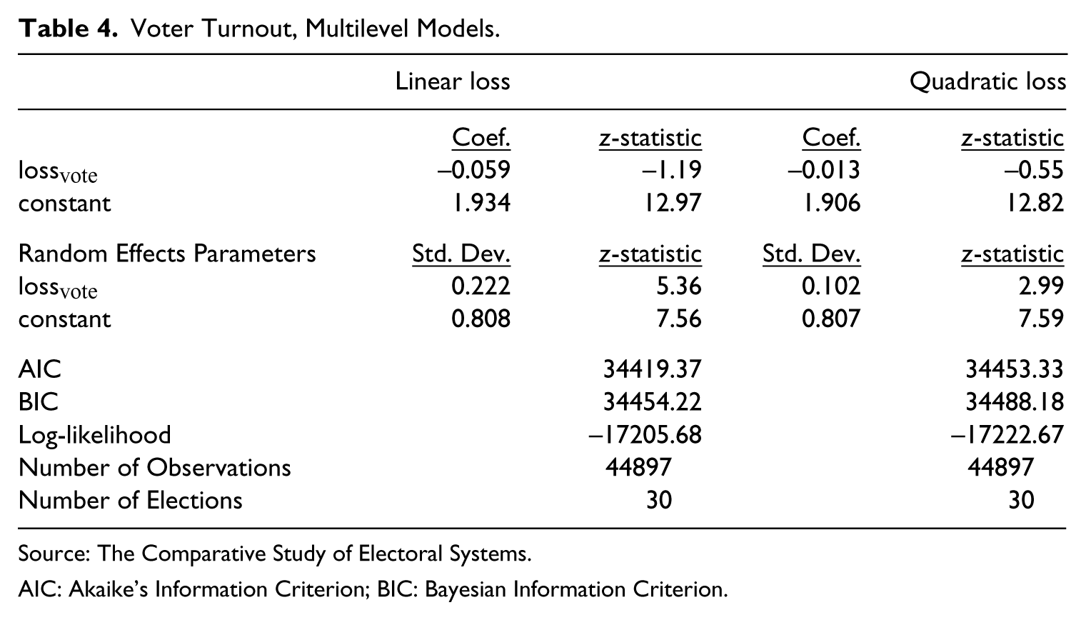
Source: The Comparative Study of Electoral Systems.

AIC: Akaike’s Information Criterion; BIC: Bayesian Information Criterion

In both Tables 3 and 4, the estimated standard deviations of the coefficients on loss_inc and loss_vote are significantly different from zero, as indicated by the associated z-statistics. This indicates that there is significant variation in the effect of loss across elections, for both the linear and quadratic formulations. In other words, the multilevel models capture the variation in the β coefficients on loss illustrated in Figures 2 and 3.

The multitude of empirical tests presented here lead to three conclusions of importance for those conducting research guided by the spatial proximity model of voter utility. First, the relationship between loss and voter behavior, whether formulated linearly or quadratically, varies markedly across countries and elections. Second, on average, over all countries, linear loss outperforms quadratic loss in regard to voter choice. Third, on average, over all countries, the linear loss function also outperforms the quadratic loss function in terms of voter turnout. In Appendices 1 and 2, I reanalyze the models depicted in Tables 1 –4 and Figures 1 and 2 using aggregated and raw individual-level placements of parties, rather than expert provided placements. Results are very similar in both cases.

7. Conclusion

The proximity model of voting does not perfectly predict vote choice or turnout. In fact, proximity behavior may not occur at all because of individual-or societal-level factors that make the model difficult to follow or alter the relative importance of ideological criteria to the voter (e.g. Boatright, 2008; Kedar, 2005; Singh, 2010; Wessels and Schmitt, 2008). As such, it is important for researchers to both be aware of variation in the applicability of the proximity model when conducting cross-national research and understand how to best model voter utility when applying the proximity model. An understanding of voter utility functions is also important to those who seek elected office, as a candidate seeking to take a stance on a given issue will want to understand ‘how steeply utility functions drop off with increasing distance from the most preferred points’ (Page, 1976: 749).

A loss function maps this ‘drop off’ in utility, capturing the decrease associated with an outcome as the location of that outcome deviates from a voter’s ideal point. While linear loss assumes a constant utility decline as distance increases, quadratic loss assumes that this decline proceeds at an increasing rate as alternatives increase in ideological distance. The quadratic loss formulation thus assumes that alienation is a strong determinant of voting behavior—a problematic assumption given previous work establishing a nonexistent or minimal alienation effect (e.g. Guttman et al., 1994; Peress, 2011; Plane and Gershtenson, 2004; Thurner and Eymann, 2000; Weisberg and Grofman, 1981). The quadratic loss formulation also clashes with psychology research demonstrating that humans tend to differentiate among items in linear terms (e.g. Dawes and Corrigan, 1974). Thus, the choice between these two functions in the study of voting behavior is likely not without consequence.

The broad cross-national empirical comparison here uncovers an advantage for the linear loss function, which provides for models that better reproduce voter behavior. As assigning utility values based on linear loss better captures intuition, and modeling utility as a quadratic function of distance is appropriate only if such a formulation is clearly demonstrated to have a better model-to-data fit than linear loss (Ordeshook, 1986), the recommendation provided here is that researchers, as a default, operationalize utility using a linear loss function if they are without clear guidance to do otherwise.

The power of positive, empirical, and experimental models of voting behavior increases when researchers have a fuller understanding of voter utility. Future studies, whether purely formal, observational, or experimental, can thus benefit from this guidance on the modeling of utility functions. There is no reason to discard the linear loss function in lieu of the more complicated quadratic, barring the existence of compelling evidence to do so.

Footnotes

Appendix 1: Aggregated individual party placements

Party positions are also obtainable from individuals’ perceptions of the political parties, as the CSES implores respondents to locate political parties on the 0 to 10 continuum. Some research has found problems with this approach. First, respondents may place their most-preferred party unduly close to their own position (Adams et al., 2005). Additionally, respondents may ensure that their placements correspond to the proximity voting criterion (Boatright, 2008). Nevertheless, to provide as complete an empirical testing as possible, I recode party positions using individual placements.

I create these placements using the averaged party placements of respondents who are at least college-educated. These respondents are presumably most knowledgeable about politics—though the link between education and political knowledge is indirect (e.g. Jerit et al., 2006; Kingston et al., 2003)—and are therefore most capable of assessing political stimuli. In fact, Alvarez and Franklin (1994) show that uninformed voters are most likely to place parties they are unfamiliar with in the middle of a scale rather than providing no placement. My approach is similar to the strategies of Golder and Stramski (2010) and Alvarez and Nagler (2004), who use only the placements of those in the most educated two-fifths of respondents. Assuming the errors individuals make when placing parties are random (a strong assumption), this averaging process should cancel out error and produce reliable placements. I re-measure each loss variable using these aggregated individual party placements and re-estimate each model in this study. Results are provided in Tables 5 –8 and Figures 4 and 5.

Overall findings from the pooled and election-by-election logit models are very similar with the use of the aggregated individual party placements. First, it is apparent that the effect of loss on voter behavior again varies substantially across elections (Figures 4 and 5). Second, in terms of model fit, the linear loss function outperforms the quadratic loss function when incumbent voting is taken as the dependent variable in a pooled logit (Table 5). Third, the linear loss function also outperforms the quadratic when turnout is the outcome variable in a pooled logit (Table 6). For both incumbent voting and turnout, Akaike weights indicate that the linear loss models are better fitting with a probability close to 1.0.

The multilevel incumbent voting models tell a similar story in regard to incumbent voting, with the linear loss function leading to a better model fit than the quadratic (Table 7). Akaike weights indicate that the linear loss model is better fitting than the quadratic with a probability close to 1.0. However, when turnout is the dependent variable, the coefficient on each conceptualization of the loss_vote variable indicates an unexpectedly and, quite implausibly, positive effect of distance from the nearest party on the propensity to vote, though neither obtains statistical significance (Table 8). Aside from these counterintuitive estimates, the evidence provided here again provides that the linear conceptualization of utility loss provides for better-fitting models of voter behavior.

Appendix 2: Perceived individual party placements

Despite the concerns about employing the perceived party placements of individuals put forth in Appendix 1, much extant research does, in fact, use such perceptions to measure the distance between individuals and parties. As such, I also use this method of distance calculation and re-measure each loss variable using these placements. I then use these new variables to again re-estimate each model in this study.

The sample size drops to 36,314 and 42,246 for the incumbent voting and turnout models, respectively, as many of the surveyed individuals did not locate parties. Results from the pooled logit models indicate that the linear loss specification outperforms the quadratic specification for both incumbent voting (Table 9) and voter turnout (Table 10). For both dependent variables, Akaike weights indicate that the linear loss models are better fitting with a probability close to 1.0. Figures 6 and 7 depict the election-specific estimations, which again show variation in the effect of loss across elections for both the incumbent voting and turnout models.

Results from the multilevel models indicate that the linear loss specification outperforms the quadratic specification for incumbent voting (Table 11), and Akaike weights indicate that the linear loss incumbent voting model is the better fitting model with a probability close to 1.0. Alternatively, for the turnout models (Table 12), the AIC and BIC values for the linear loss specification are higher, indicating a worse fit, and Akaike weights indicate that the probability that the linear loss specification is the better fitting of the two models is just 0.22. Still, there is overwhelming evidence from the empirical exercises conducted in this paper in favor of linear loss.

Acknowledgements

The author would like to thank Robert N Lupton for helpful comments.

Notes

References

Abramowitz

(1980) A comparison of voting for US Senator and Representative in 1978. American Political Science Review 74(3): 633–640.

Adams

Merrill

III (2003) Voter turnout and candidate strategies in American elections. Journal of Politics 65(1): 161–189.

Adams

Dow

Merrill

(2006) The political consequences of alienation-based and indifference-based voter abstention: applications to presidential elections. Political Behavior 28(1): 65–86.

Adams

Merrill

Grofman

(2005) A Unified Theory of Party Competition: A Cross-National Analysis Integrating Spatial and Behavioral Factors. Cambridge, UK: Cambridge University Press.

Alvarez

Franklin

(1994) Uncertainty and political perceptions.Journal of Politics 56(3): 671–88.

Alvarez

Nagler

(2004) Party system compactness: measurement and consequences. Political Analysis 12(1): 46–62.

Bartels

(1986) Issue voting under uncertainty: an empirical test. American Journal of Political Science 30(4): 709–728.

Blais

Labbé St-Vincent

Laslier

J-F

. (2011) Strategic vote choice in one round and two round elections. Political Research Quarterly 64(3): 637–45.

Blais

Nadeau

Gidengil

. (2001) The formation of party preferences: testing the proximity and directional models. European Journal of Political Research 40(1): 81–91.

10.

Boatright

(2008) Who are the spatial voting violators? Electoral Studies 27(1): 116–125.

11.

Bobbio

(1996) Left Right: The Significance of a Political Distinction. Cambridge, UK: Polity Press.

12.

Brehmer

Berndt

(1987) Note on subjects’ hypotheses in multiple-cue probability learning. Organizational Behavior and Human Decision Processes 40(3): 323–329.

13.

Brody

Page

(1973) Indifference, alienation and rational decisions: the effects of candidate evaluations on turnout and the vote. Public Choice 15(1): 1–17.

14.

Budge

Ezrow

McDonald

(2010) Ideology, party factionalism and policy change: an integrated dynamic theory. British Journal of Political Science 40(4): 781–804.

15.

Burnham

Anderson

(2002) Model Selection and Multimodel Inference: A Practical Information-theoretic Approach. New York: Springer.

16.

Calvo

Hellwig

(2011) Centripetal and centrifugal incentives under different electoral systems. American Journal of Political Science 55(1): 28–41.

17.

Campbell

Converse

Miller

Stokes

(1960) The American Voter. New York: John Wiley.

18.

Converse

(1966) The concept of the normal vote. In: Campbell

Converse

Miller

. (eds) Elections and the Political Order. New York: John Wiley & Sons, Inc.

19.

Cox

(1990) Centripetal and centrifugal incentives in electoral systems. American Journal of Political Science 34(4): 903–935.

20.

Davis

Hinich

Ordeshook

(1970) An expository development of a mathematical model of the electoral process. American Political Science Review 64(2): 426–448.

21.

Dawes

Corrigan

(1974) Linear models in decision making. Psychological Bulletin 81(2): 93–106.

22.

Downs

(1957) An Economic Theory of Democracy. New York: Harper Collins.

23.

Duch

May

Armstrong

II (2010) Coalition-directed voting in multiparty democracies. American Political Science Review 104(4): 698–719.

24.

Einhorn

Gonedes

(1971) An exponential discrepancy model for attitude evaluation. Behavioral Science 16(3): 152–157.

25.

Enelow

Hinich

(1981) A new approach to voter uncertainty in the Downsian spatial model. American Journal of Political Science 25(3): 483-493.

26.

Enelow

Hinich

(1982) Nonspatial candidate characteristics and electoral competition. Journal of Politics 44(1): 115–30.

27.

Enelow

Hinich

(1984a) Probabilistic voting and the importance of centrist ideologies in democratic elections. Journal of Politics 46(2): 459–478.

28.

Enelow

Hinich

(1984b) The Spatial Theory of Voting. New York: Cambridge University Press.

29.

Funk

(1999) Bringing the candidate into models of candidate evaluation. Journal of Politics 61(3): 700–720.

30.

Gabel

Huber

(2000) Putting parties in their place: inferring party left-right ideological positions from party manifestos data. American Journal of Political Science 44(1): 94–103.

31.

Gilljam

(1997) The directional theory under the magnifying glass: a reappraisal. Journal of Theoretical Politics 9(1): 5–12.

32.

Golder

Stramski

(2010) Ideological congruence and electoral institutions. American Journal of Political Science 54(1): 90–106.

33.

Grynaviski

Corrigan

(2006) Specification issues in proximity models of candidate evaluation (with issue importance). Political Analysis 14(1): 393–420.

34.

Guttman

Hilger

Shachmurove

(1994) Voting as investment vs. voting as consumption: new evidence. Kyklos 47(2): 197–207.

35.

Hammond

Summers

(1965) Cognitive dependence on linear and nonlinear cues. Psychological Review 72(3): 215–224.

36.

Hastie

Dawes

(2010) Rational Choice in an Uncertain World: The Psychology of Judgement and Decision Making. Thousand Oaks: Sage.

37.

Hotelling

(1929) Stability in competition. Economic Journal 39(153): 41–57.

38.

Jackman

(1987) Political institutions and voter turnout in the industrial democracies. American Political Science Review 81(2): 405–423.

39.

Jerit

Barabas

Bolsen

(2006) Citizens, knowledge, and the information environment. American Journal of Political Science 50(2): 266–282.

40.

Jessee

(2009) Spatial voting in the 2004 presidential election. American Political Science Review 103(1): 59–81.

41.

Jessee

(2010) Partisan bias, political information and spatial voting in the 2008 presidential election. Journal of Politics 72(2): 327–340.

42.

Kedar

(2005) When moderate voters prefer extreme parties: policy balancing in parliamentary elections. American Political Science Review 99(2): 185–199.

43.

Kingston

Hubbard

Lapp

. (2003) Why education matters. Sociology of Education 76(1): 53–70.

44.

Krämer

Rattinger

(1997) The proximity and the directional theories of issue voting: comparative results for the US and Germany. European Journal of Political Research 32(1): 1–29.

45.

Lachat

(2008) The impact of party polarization on ideological voting. Electoral Studies 27(4): 687–698.

46.

Lin

Enelow

Dorussen

(1999) Equilibrium in multicandidate probabilistic spatial voting. Public Choice 98(1–2): 59–82.

47.

Lupia

(1994) The effect of information on voting behavior and electoral outcomes: an experimental study of direct legislation. Public Choice 78(1): 65–86.

48.

McKelvey

Ordeshook

(1985) Elections with limited information: a fulfilled expectations model using contemporaneous poll and endorsement data as information sources. Journal of Economic Theory 36(1): 55–85.

49.

McKelvey

Wendell

(1976) Voting equilibria in multidimensional choice spaces. Mathematics of Operations Research 1(2): 144–158.

50.

Merrill

III Adams

(2001) Computing Nash equilibria in probabilistic, multiparty spatial models with nonpolicy components. Political Analysis 9(4): 347–361.

51.

Morton

(1993) Incomplete information and ideological explanations of platform divergence. American Political Science Review 87(2): 382–392.

52.

Norris

(2004) Electoral Engineering: Voting Rules and Political Behavior. Cambridge, UK: Cambridge University Press.

53.

Olson

Gale

(1968) Spatial theory and human behavior. Papers and Proceedings of the Regional Science Association 21(1): 229–242.

54.

Ordeshook

(1986) Game Theory and Political Theory. Cambridge, UK: Cambridge University Press.

55.

Page

(1976) The theory of political ambiguity. American Political Science Review 70(3): 742–752.

56.

Palfrey

Rosenthal

(1983) A strategic calculus of voting. Public Choice 41(1): 7–53.

57.

Peress

(2011) Securing the base: electoral competition under variable turnout. Public Choice 148(1): 87–104.

58.

Pierce

(1997) The directional theory of issue voting: directional versus proximity models: verisimilitude as the criterion. Journal of Theoretical Politics 9(1): 61–74.

59.

Plane

Gershtenson

(2004) Candidates’ ideological locations, abstention, and turnout in US midterm Senate elections. Political Behavior 26(1): 69–93.

60.

Poole

Rosenthal

(1985) A spatial model for legislative roll call analysis. American Journal of Political Science 29(2): 357–384.

61.

Poole

Rosenthal

(1997) Congress: a Political-Economic History of Roll Call Voting. Oxford: Oxford University Press.

62.

Riker

Ordeshook

(1968) A theory of the calculus of voting. American Political Science Review 62(1): 25–42.

63.

Riker

Ordeshook

(1973) An Introduction to Positive Political Theory. Englewood Cliffs, NJ: Prentice Hall.

64.

Shapiro

(1969) Rational political man: A synthesis of economic and social-psychological perspectives. American Political Science Review 63(4): 1106–1119.

65.

Singh

(2010) Contextual Influences on the decision calculus: a cross-national examination of proximity voting. Electoral Studies 29(3): 425–434.

66.

Singh

(2011) Contradictory calculi: differences in individuals’ turnout decisions across electoral systems. Political Research Quarterly 64(3): 646–655.

67.

Thurner

(2000) The empirical application of the spatial theory of voting in multiparty systems with random utility models. Electoral Studies 19(4): 493–517.

68.

Thurner

Eymann

(2000) Policy-specific alienation and indifference in the calculus of voting: a simultaneous model of party choice and abstention. Public Choice 102(1–2): 51–77.

69.

Weisberg

Grofman

(1981) Candidate evaluations and turnout. American Politics Research 9(2): 197–219.

70.

Wessels

Schmitt

(2008) Meaningful choices, political supply, and institutional effectiveness. Electoral Studies 27(1): 19–30.

71.

Westholm

(1997) Distance versus direction: the illusory defeat of the proximity theory of electoral choice. American Political Science Review 91(4): 865–883.

72.

Williams

(1994) Spatial elections with endorsements and uninformed voters: some laboratory experiments. Public Choice 80(1–2): 1–8.

73.

Wittman

(1973) Parties as utility maximizers. The American Political Science Review 67(2): 490–498.

74.

Wittman

(2007) Candidate quality, pressure group endorsements and the nature of political advertising. European Journal of Political Economy 23(2): 360–378.